PHYSICAL REVIEW B 73, 024420 共2006兲
Theory for nucleation at an interface and magnetization reversal of a two-layer nanowire Peter N. Loxley* and Robert L. Stamps School of Physics, University of Western Australia, 35 Stirling Highway, Crawley, WA 6009 Australia 共Received 16 June 2005; revised manuscript received 29 November 2005; published 25 January 2006兲 Nucleation at the interface between two adjoining regions with dissimilar physical properties is investigated using a model for magnetization reversal of a two-layer ferromagnetic nanowire. Each layer of the nanowire is considered to have a different degree of magnetic anisotropy, representing a hard magnetic layer exchangecoupled to a softer layer. A magnetic field applied along the easy axis causes the softer layer to reverse, forming a domain wall close to the interface. For small applied fields this state is metastable and complete reversal of the nanowire takes place via activation over a barrier. A reversal mechanism involving nucleation at an interface is proposed, whereby a domain wall changes in width as it passes from the soft layer to the hard layer during activation. Langer’s statistical theory for the decay of a metastable state is used to derive rates of magnetization reversal, and simple formulas are found in limiting cases for the activation energy, rate of reversal, and critical field at which the metastable state becomes unstable. These formulas depend on the anisotropy difference between each layer, and the behavior of the reversal rate prefactor is interpreted in terms of activation entropy and domain-wall dynamics. DOI: 10.1103/PhysRevB.73.024420
PACS number共s兲: 75.60.Jk, 64.60.Qb, 64.60.My, 75.60.Ch
I. INTRODUCTION
During the process of nucleation, the decay of a metastable state is initiated by the formation of a spatially localized region known as a nucleus of critical size. In many realistic situations nucleation occurs at a nonuniformity or defect, such as an irregularity in a sample. One common type of defect is the interface which forms between two adjoining regions with dissimilar physical properties. Assuming both regions are reasonably strongly coupled together, a phase transition that takes place in one region will encounter this defect before spreading into the adjoining region. The strength of the defect depends on the difference in the physical properties of each region. Artificially fabricated magnetic nanowires provide a unique opportunity to investigate nucleation within a onedimensional system. Over the past decade, thermally activated magnetization reversal has been thoroughly investigated for homogeneous nanowires and elongated nanoparticles both experimentally1–4 and theoretically,5–7 and the thermal stability of the magnetization has been described using a model that includes the nucleation of solitonantisoliton pairs.5,6 More recently, attention has turned towards the fabrication of nanowires with controlled defects8 and alternating magnetic layers.2,4 Magnetization reversal of tailor-made geometries with nonuniform magnetic properties has been investigated for the case of submicron wires with necks, pads, and junctions9 and for thin films with alternating hard and soft magnetic layers such as those found in exchange-spring materials.10–17 The purpose of the present study is to investigate nucleation at an interface using a model for thermally activated magnetization reversal of a two-layer nanowire. This model is closely related to the double sine-Gordon model, which is one of the simplest and most generally used models for describing nucleation. For this reason our results carry over to a wide variety of systems comprised of two adjoining re1098-0121/2006/73共2兲/024420共14兲/$23.00
gions with dissimilar physical properties. Each layer of the nanowire is assumed only to differ in the strength of the uniaxial magnetic anisotropy, representing hard and soft magnetic layers, and the layers are also assumed to be exchange-coupled across the joining interface. This leads to a magnetic defect consisting of a step change in the anisotropy strength. It is possible to control the strength of the defect by varying the choice of each layer, allowing thermal stability to be tailored to suit potential applications. The choice of a nanowire geometry allows us to provide a detailed treatment of the reversal mechanism near the defect without having to deal with complicated reversal modes typically found in bulk materials. The important simplification is in the form of the energy due to the demagnetizing field. For a cylindrical nanowire with a diameter below the magnetic exchange length, the formation of nonuniform magnetic configurations over the wire cross section becomes less likely, as the cost in exchange energy outweighs the reduction in demagnetizing energy.18–23 The energy of magnetic configurations can then be treated as having an approximately onedimensional dependence, varying along the nanowire. Conversely, for larger-diameter wires the curling mode replaces coherent rotation and nonuniform vortexlike states may form over the wire cross section.18–23 A magnetic field applied along the easy axis of a twolayer nanowire causes the magnetization of the softer layer to reverse orientation, forming a domain-boundary wall close to the interface between the layers as shown in Fig. 1. For small applied fields this wall becomes trapped near the interface and complete reversal of the nanowire proceeds only after activation over an energy barrier takes place 共see Fig. 2兲. Although it is tempting to describe this activation as a domain-wall depinning process 共where only the position of the wall center changes兲, we show that this approach misses much of the crucial behavior. In particular, the wall configuration is found to change completely as the wall crosses the interface, partly to accommodate a change in wall width. We
024420-1
©2006 The American Physical Society
PHYSICAL REVIEW B 73, 024420 共2006兲
PETER N. LOXLEY AND ROBERT L. STAMPS
FIG. 1. Geometry of the model nanowire consists of two exchange-coupled magnetic layers with different uniaxial anisotropy constants K1 共soft layer兲 and K2 共hard layer兲, such that K2 ⬎ K1. A weak magnetic field H applied along the easy axis leads to a metastable domain wall formed within the soft layer.
are therefore led to consider activation as the nucleation of a domain wall in the hard layer. The rate of thermal activation is given by the well-known Van ’t Hoff–Arrhenius law I = I 0e −Ea ,
共1兲
where the activation energy Ea is the height of the lowestenergy barrier separating a metastable minimum from a lower-energy minimum,  is the inverse temperature, and the prefactor I0 depends on the dynamics of the barrier crossing, as well as the entropy of the activated state compared with that of the metastable state.24 The exponential factor in Eq. 共1兲 implies that thermal activation is a rare event when Ea Ⰷ 1, meaning that it takes place over time scales much longer than those in I0 characterizing the system dynamics. This makes computer simulation of activated events time consuming, and because the dynamics is stochastic, many simulations are required in order to find the average behavior. Instead we use a statistical theory of metastable decay originally due to Langer.25,26 For the simple geometry of a two-layer nanowire this allows us to find analytic expressions for Ea and I0 in the important limiting cases. The structure of the paper is as follows. In Sec. II, the model and assumptions are outlined and the energy of magnetic configurations is shown to have the form of the double sine-Gordon model with out-of-plane deviations and a step defect. A reversal mechanism involving a domain wall that changes in width during activation is proposed in Sec. III, and explicit expressions are found for the metastable and unstable magnetic configurations. The critical field at which
FIG. 2. A domain wall centered at x = x0 in a two-layer nanowire with interface at x = 0 is shown in 共a兲, while the energy of the wall as a function of wall position is shown in 共b兲. This energy is seen to have a local minimum when the wall is centered in the soft layer 共x ⬎ 0兲 near the interface and a local maximum when centered in the hard layer 共x ⬍ 0兲 near the interface.
the metastable configuration becomes unstable 共the zerotemperature coercive field兲 is also found, and limiting expressions for Ea are given. In Sec. IV, the energy of small deviations in the equilibrium configurations is considered and modes corresponding to infinitesimal wall rotations and wall translations are identified. Formulas for the rate of thermally activated reversal are derived, and the behavior of I0 is interpreted in terms of domain wall dynamics and activation entropy, where mode trapping from soliton theory is seen to play a role. The rate of reversal is explicitly calculated for a partly annealed FePt nanowire in Sec. V. II. MODEL
A cylindrical geometry is assumed for our nanowire, and one layer has magnetic anisotropy constant K1, while the other has K2, such that K2 ⬎ K1. The layer with K2 will be referred to as the hard layer and K1 as the soft layer. The anisotropy is considered to be of uniaxial nature, with the easy axis coinciding with the longitudinal axis of the nanowire, and a magnetic field H is applied along the easy axis as shown in Fig. 1. It is also assumed that the exchange interaction between magnetic moments extends across the interface between the hard and soft layers as, for example, found in exchange-spring materials.10–17 Some models allow for a reduction in exchange at the interface to allow for the growth of nonideal interfaces.16,17 Here, however, we assume that exchange coupling at the interface is close to that in the bulk. Adopting a classical continuum model commonly used in micromagnetics and choosing the easy axis to be the x direction in Cartesian coordinates, the magnetization is described by the vector m共x兲 which can vary in orientation along the nanowire and obeys 兩m 兩 = 1. The energy of possible magnetic configurations is assumed to have the form E = Ar
冕
L/2
−L/2
再冉 冊
dx A
dm dx
2
冎
− K共x兲m2x − 0M sHmx ,
共2兲
for a nanowire of length L and cross-section area Ar. The first term in Eq. 共2兲 describes the classical continuum counterpart of the exchange interaction, while the second and third terms describe an easy-axis anisotropy in the x direction and a magnetic field applied along the easy axis. The magnetization naturally prefers to align along the easy axis in the direction of the applied magnetic field, and spatially uniform configurations are preferred over nonuniform ones due to the exchange coupling between neighboring magnetic moments. The hard and soft layers are modeled by allowing the anisotropy constant K to vary with position along the nanowire, and if the interface between the two layers is sharp and well defined over the length scale of a domain-wall width, K共x兲 can be chosen to have a steplike variation: K共x兲 = 1 − ␣U共x兲, K2 where U共x兲 is the unit step function, obeying
024420-2
共3兲
PHYSICAL REVIEW B 73, 024420 共2006兲
THEORY FOR NUCLEATION AT AN INTERFACE AND…
U共x兲 =
再
1,
x ⬎ 0,
0,
x ⬍ 0,
for an interface at x = 0, and the constant ␣ depends on the difference in anisotropy strength between the hard and soft layers:
␣=
K2 − K1 . K2
共4兲
The anisotropy constants contain the effects of both crystalline and shape anisotropies, the latter which Braun demonstrated to be of the form 0M s2 / 4 for nonuniform configurations in thin nanowires,18 as the nonlocal contribution to the demagnetizing energy becomes small in this case. The central assumption of our model is that the magnetization only varies over the length of the nanowire; there is no change in orientation over the wire cross section. This onedimensional approximation is expected to hold whenever the nanowire diameter d satisfies d ⬍ ␦ex, where ␦ex = 冑A / 0M s2 is the magnetic exchange length.18 Below this the cost in exchange energy for m to deviate from a uniform configuration outweighs the possible reduction in energy from the demagnetizing field. Values of the critical diameter ␦ex range between 5 and 10 nm for common ferromagnetic materials such as Co, Ni, and Fe.27 The length, energy, and time scales we are interested in are given by the width ␦w and energy 2⌬w of a domain wall in the hard layer and the time of precession of a magnetic moment in the hard layer, where
␦w ⬅
冑
A , K2
⌬w ⬅ 2Ar冑AK2,
⬅ 共1 + ␥2兲
Ms , 2 ␥ GK 2 共5兲
with ␥G the gyromagnetic ratio and ␥ the dimensionless damping constant from the Landau-Lifshitz-Gilbert equation describing magnetization dynamics 共Sec. IV B兲. The constraint 兩m 兩 = 1 can be satisfied by introducing spherical-polar coordinates, whereupon the magnetization vector becomes m = 共sin cos , sin sin , cos 兲. In terms of sphericalpolar coordinates and the characteristic length and energy scales defined above, the energy expression given by Eq. 共2兲 is then E=
冕
L/2
−L/2
dx
再 冋冉 冊 1 2
d dx
2
+ sin2
冉 冊册 d dx
2
冎
+ V − ␣U共x兲Vd , 共6兲
where V = Vd − h sin cos ,
1 Vd = − sin2 cos2 , 2
共7兲
This corresponds to nanowires which are longer than the domain wall width ␦w. The energy expression given by Eqs. 共6兲 and 共7兲 reduces to the double sine-Gordon model with a step defect upon setting = / 2. Sine-Gordon models have been used extensively for describing phase transitions and domain walls in a wide variety of systems, and the relevant solutions are also known as kinks, solitons, or instantons. III. REVERSAL MECHANISM
The energy of a domain wall moving through a two-layer nanowire can be described using the expression given by Eqs. 共6兲 and 共7兲. A single planar domain wall is represented by 共 , 兲 = 共s , / 2兲, where the function s共x兲 is given by
s共x兲 = 2 arctan e−共x−x0兲 ,
共9兲
with x0 describing the position of the center of the wall as shown in Fig. 2共a兲. Inserting the relations s⬘ = sin s, sin s = sech共x − x0兲, and cos s = tanh共x − x0兲 which follow from Eq. 共9兲 into Eq. 共6兲, then taking the limit as L → ⬁ before integrating, yields an expression for the energy given by Es ⬀ 4hx0 − ␣ tanh x0
共10兲
and is plotted in Fig. 2共b兲. It is clear from Eq. 共10兲 or Fig. 2共b兲 that two energy extrema exist, one on either side of the interface at x = 0. These extrema result from a competition between the applied field h and the anisotropy difference ␣. A domain wall decreases in Zeeman energy as it moves from positive values of x to less positive values, and the magnetic moments correspondingly flip into the direction of the applied field. However, a wall in the soft layer takes less energy to form than a wall in the hard layer. We propose the following reversal mechanism for a twolayer nanowire. In an applied field the soft layer reverses before the hard layer, introducing a domain wall into the soft layer. Under the influence of the applied field this wall moves towards the interface until reaching the energy minimum shown in Fig. 2共b兲. The magnetization is now metastable, and the system can be thermally activated over a barrier. After this occurs the wall moves through the hard layer and reverses the orientation of the magnetization. While this mechanism may be qualitatively correct, there is a problem with the preceding analysis. A fundamental property of domain walls is that the wall width depends on the anisotropy strength. A wall in a relatively soft layer is expected to be wider than a wall in a harder layer, yet in this reversal mechanism the wall maintains a fixed width when moving between the hard and soft layers. In order to properly describe reversal we must therefore find the true energy extremum configurations.
and the dimensionless field h is given by
0 M sH . h= 2K2
A. Energy extremum configurations
共8兲
Here we will not be concerned with effects due to the ends of a nanowire and the limit L → ⬁ is taken in the final result.
The energy extremum configurations of Eq. 共6兲 can be found by solving the Euler-Lagrange equations. The equation corresponding to ␦E / ␦ = 0 is solved by = / 2; then, ␦E / ␦ = 0 becomes
024420-3
PHYSICAL REVIEW B 73, 024420 共2006兲
PETER N. LOXLEY AND ROBERT L. STAMPS
FIG. 3. Superimposing the curves V1 and V2 leads to the two intersection points + and − seen in 共a兲. Analog particle trajectories lying between = and = 0 can be joined together at either = − or = +, leading to the configurations seen in 共b兲 and 共c兲, respectively.
−
d 2 + V⬘共兲 − ␣U共x兲Vd⬘共兲 = 0, dx2
Ⲑ
共11兲
Ⲑ
with V共兲 = − 1 2 cos2 − hcos and Vd共兲 = − 1 2 cos2 . The step function U共x兲 is discontinuous at x = 0, so we derive a consistency condition to be satisfied by at this point. Integrating Eq. 共11兲 over 共− , 兲, then letting → 0, yields
冏 冏 冏 冏 d dx
=
x=0+
d dx
共12兲
, x=0−
since U共x兲 describes only a finite jump. Solutions to Eq. 共11兲 therefore have continuous first derivatives at the interface. Integrating the Euler-Lagrange equation once yields
冉 冊
1 d 2 dx and
2
− V共兲 + ␣Vd共兲 = C1,
冉 冊
1 d 2 dx
2
− V共兲 = C2,
x ⬎ 0,
x ⬍ 0,
共13兲
共14兲
where C1 and C2 are the constants of integration. The boundary conditions satisfied by the domain wall in Fig. 2 are 共x → − ⬁ 兲 = , 共x → ⬁ 兲 = 0, and ⬘共x → ± ⬁ 兲 = 0, from which C1 = 1 2 共1 − ␣兲 + h and C2 = 1 2 − h are found. All possible solutions to Eqs. 共13兲 and 共14兲 can be found by considering an analog problem in particle mechanics: namely, the conservative motion of a classical particle in a one-dimensional 共1D兲 potential. Consider the two potentials V1共兲 = −V + ␣Vd − C1 and V2共兲 = −V − C2, which are shown in Fig. 3共a兲. Now consider a particle which initially sits on the peak at = 0 of the curve V1 in Fig. 3共a兲 with zero kinetic energy. An infinitesimal nudge causes this particle to roll down V1 away from the unstable equilibrium, slowly at first, but picking up speed as it heads towards the minimum. According to Eqs. 共13兲 and 共14兲, a second particle which begins
Ⲑ
Ⲑ
FIG. 4. Field dependence of the energy extremum configura+ − tions w and w . In the limit as h → 0, both walls are far from the interface at x = 0 关shown in 共a兲 and 共b兲兴 and the wall in the soft layer 共x ⬎ 0兲 is clearly wider than the wall in the hard layer 共x ⬍ 0兲. For 0 ⬍ h ⬍ hc both walls move towards the interface 关shown in 共c兲 and 共d兲兴, while for h → hc both walls are given by the same configuration 关shown in 共e兲 and 共f兲兴.
at = on V2 with zero kinetic energy and follows V2 after being nudged will have the same total energy as the first particle following V1. If the particle “coordinate” is and the “time” is x, this means that the kinetic energy T = 1 2 共d / dx兲2 of each particle must be equal at either of the two intersection points where V1 = V2. Both particle trajectories can therefore be joined together at either + or −, generating two possible solutions to Eqs. 共13兲 and 共14兲 which satisfy the consistency condition, Eq. 共12兲. These are shown in Figs. 3共b兲 and 3共c兲. The intersection points + and − can be found with the help of Eq. 共7兲, yielding
Ⲑ
sin ± = 2
冑
h . ␣
共15兲
This equation is guaranteed to have two solutions between 0 and if 0 ⬍ 2冑h / ␣ ⬍ 1. In other words, + and − exist over the range 0 ⬍ h ⬍ h c,
where hc =
␣ . 4
共16兲
The parameter hc corresponds to the critical field of reversal 共or zero-temperature coercive field兲 and follows directly from the form of the interface between the two layers, in this case approximated as a discontinuous step in the anisotropy.
024420-4
PHYSICAL REVIEW B 73, 024420 共2006兲
THEORY FOR NUCLEATION AT AN INTERFACE AND…
The explicit form of the solutions for the two extremum configurations can be found by integrating Eqs. 共13兲 and 共14兲 with C1 and C2, leading to
x±2
␦2
冉冑
= arccosh
where
w±共x兲
=
冦
冋冑
冒 冉
2 arctan
h+1−␣ h
2 arctan
x − x±2 h cosh 1−h ␦2
冋冑
sinh
x − x±1
冉 冊册
␦1
冊册
x ⬍ 0,
,
共17兲
where the dimensionless wall widths are given by
␦1 =
1
冑h + 1 − ␣
,
␦2 =
1
共18兲
冑1 − h ,
and the constants of integration x1 and x2 are found by re± 共x = 0兲 = ± holds, yielding quiring that w x±1
␦1
冉冑 冒 冊
= − arcsinh
h+1−␣ h
w±共x兲
=
再
共19兲
A± ,
1±
2 arctan e
关共x−x±2 兲/␦2−R2兴
−关共x−x±2 兲/␦2+R2兴
+ 2 arctan e
+
h→0
−
− lim w = 2 arctan e−关共x−x1 兲/␦1−R1兴 .
共24兲
+ describes a domain wall comThe solution given by w − describes a pletely formed within the hard layer, while w wall completely formed within the soft layer. It is now seen that when a metastable wall in the soft layer becomes thermally activated, the wall width changes from ␦1 to ␦2 as the wall moves into the hard layer. The change in wall width can be clearly seen in plots of Eq. 共17兲 for small field as shown in Figs. 4共a兲 and 4共b兲. As h → 0, each extremum configuration is far from the interface
.
共21兲
h = sech2R2 .
共22兲
The parameter R1 allows Eq. 共17兲 for x ⬎ 0 to be written as the superposition of two walls of the form of Eq. 共9兲 separated by a distance of 2␦1R1. Similarly, the parameter R2 allows Eq. 共17兲 for x ⬍ 0 to be written as the superposition of one wall of the form of Eq. 共9兲 and another similar solution but with −x, separated by a distance of 2␦2R2, yielding
±
+ = 2 arctan e−关共x−x2 兲/␦2+R2兴, lim w
h 1− hc
h = cosech2R1, 共1 − ␣兲
±
Ⲑ
h hc
共20兲
+ Choosing A+ in x±1 and x±2 leads to w , the unstable wall in the hard layer shown in Fig. 3共c兲, while choosing A− leads to w−, the metastable wall in the soft layer shown in Fig. 3共b兲. The two extremum energy configurations can be interpreted more intuitively by rewriting Eq. 共17兲 as a superposition of domain walls of the form given by Eq. 共9兲. This is done by introducing two new parameters R1 and R2, defined by
2 arctan e−关共x−x1 兲/␦1−R1兴 + 2 arctan e−关共x−x1 兲/␦1+R1兴 ,
This form of Eq. 共17兲 can be used to show that the energy extremum configurations describe a domain wall that changes in width during activation. To do this we consider Eq. 共21兲 in the limit h → 0, from which we find A+ = 冑h / ␣ and A− = 冑␣ / h, leading to x+1 / ␦1 = ln h, x+2 / ␦2 = const, x−1 / ␦1 = const, and x−2 / ␦2 = −ln h. In this limit we also have R1 = R2 ± = − 1 2 ln h. Using these values in Eq. 共23兲 for w leads to
h→0
A± =
x ⬎ 0,
,
冑 冑
冊
1−h A± , h
,
x ⬎ 0, x ⬍ 0.
共23兲
and the wall in the soft layer is wider than the wall in the hard layer. As h increases, each wall moves closer to the interface, as shown in Figs. 4共c兲 and 4共d兲. In the limit as the field approaches the critical field hc, both walls are given by the same configuration: a single wall centered at the interface as shown in Figs. 4共e兲 and 4共f兲. This last case represents a metastable configuration becoming unstable, and reversal of the magnetization can proceed in the absence of activation. The behavior of the energy extremum configurations shown in Fig. 4 allows for the consideration of two simple limits. As h → 0, each configuration moves away from the interface and the solution simplifies to Eq. 共24兲. In the opposite limit of h → hc, both configurations are described by the same solution. These limiting cases will be used in the following work. B. Activation energy and critical field
Expressions for the activation energy and critical field can be found for the proposed reversal mechanism. From Eqs. 共4兲, 共8兲, and 共16兲, it is clear that the critical field 共or zerotemperature coercive field兲 is
024420-5
PHYSICAL REVIEW B 73, 024420 共2006兲
PETER N. LOXLEY AND ROBERT L. STAMPS
Hc =
K2 − K1 . 20 M s
For applied fields larger than Hc, the domain wall in the soft layer becomes unstable and proceeds through the hard layer and no thermal activation is required in order to reverse the magnetization of the nanowire. As the anisotropy constant K1 approaches K2, the critical field vanishes as expected. Notice, however, the surprising fact that for K1 Ⰶ K2, we get Hc = K2 / 20M s. This is only one-quarter of the anisotropy field required to reverse an uncoupled hard layer and directly results from the exchange coupling between the hard and soft layers. The activation energy of the proposed reversal mechanism is given by the difference in energy between the unstable wall in the hard layer and the metastable wall in the soft layer: + − 兲 − E共w 兲. Ea = E共w
共26兲
This expression is easy to evaluate in the limiting cases considered previously. As the applied field tends to zero the walls move away from the interface and the activation energy becomes lim Ea = 4Ar冑AK2 − 4Ar冑AK1 .
H→0
H→Hc
␦共x兲 = 兺 ii共x兲, i
+ ␦共x兲 2
共2兲 ± 兲+ = E共w Ew
␦共x兲 = 兺 piip共x兲,
1 1 i2i + 兺 ⬘ip p2i , 兺 2 i 2 i
Hi = ii,
H pip = ipip
Small deviations in each of the energy extremum configu+ − and w include both deviations ␦ in the plane of rations w a wall 共in-plane deviations兲 and deviations ␦ out of the plane of a wall 共out-of-plane deviations兲. These are defined as
共31兲
共32兲
and where H and H p are linear differential operators given by
H =
冦
H =
冦
冊 冊
冉 冉
冊 冊
x ⬎ 0,
x − x±2 1 d2 ,R2 , − 2 + 2 V− dx ␦2 ␦2
x ⬍ 0,
and
p
冉 冉
x − x±1 1 d2 ,R1 , 2 + 2 V+ dx ␦1 ␦1
−
共33兲
x − x±1 1 d2 + V ,R1 , − dx2 ␦21 ␦1
x ⬎ 0,
x − x±2 1 d2 ,R2 , − 2 + 2 V+ dx ␦2 ␦2
x ⬍ 0,
−
共34兲
with the potentials V±共,R兲 = 1 − 2 sech2共 + R兲 − 2 sech2共 − R兲 ± 2 sech共 + R兲sech共 − R兲,
A. Energy of small deviations
共30兲
i
where the energy eigenvalues i,p and eigenfunctions i,p are chosen to solve the eigenvalue equations
IV. REVERSAL RATES
The rate of thermally activated reversal not only depends on the activation energy Ea, but also on the rate prefactor I0 appearing in Eq. 共1兲. This prefactor is derived in Appendix C using Langer’s treatment for the rate of decay of a metastable state,25,26 combined with ideal gas phenomenology applied to solitons.29–31 It contains contributions from both entropy and dynamics and can be found by considering the energy of small deviations in each of the extremum configurations.
共29兲
where i and pi are the corresponding expansion coefficients describing the deviations. Since we are not simply treating domain-wall depinning, in which case only deviations in the equilibrium wall-center position would be important, we choose a complete basis that includes all possible deviations. Upon substituting Eqs. 共29兲 and 共30兲 into Eq. 共6兲, the energy of small deviations can be expressed to second order as
共28兲
The full expression for the activation energy in Eq. 共26兲 appears in Ref. 28 and decreases in a predictable manner from its maximum value at H = 0 to zero at H = Hc.
共x兲 =
and can be expanded in terms of a complete set of orthonormal eigenfunctions i,p as
共27兲
This is simply the difference in energy between a domain wall in the hard and soft layers and corresponds to the maximum possible value for the activation energy. In the opposite limit as the applied field tends towards Hc, both walls move towards the interface until they merge into the same configuration. The activation energy is then given by lim Ea = 0.
共x兲 = w±共x兲 + ␦共x兲,
共25兲
共35兲
as well as the continuity and consistency conditions i共0−兲 = i共0+兲 and i⬘共0−兲 = i⬘共0+兲. The operators H and H p are actually combinations of those found by Braun for solitonsoliton and soliton-antisoliton pairs, and we have adopted Braun’s notation here.5,6 This eigenvalue problem can be treated in much the same way as a 1D Schrödinger equation with a step potential, where the potential simplifies in the limits considered in Sec. III. The limit of small applied field is solved in Appendix A, and applied fields close to the critical field are treated in Appendix B. In the small-field limit it is found that H = H p, and the potential is shown in Fig. 5共a兲 for deviations in the unstable wall and in Fig. 5共b兲 for deviations in the metastable wall. Each potential consists of a single well of depth −2 2␦−2 2 at x ⯝ −␦2R2 共or 2␦1 at x ⯝ ␦1R1兲 due to a domain wall −2 and a step of height ␦2 − ␦−2 1 = ␣ at x = 0 due to the interface.
024420-6
PHYSICAL REVIEW B 73, 024420 共2006兲
THEORY FOR NUCLEATION AT AN INTERFACE AND…
FIG. 5. The Schrödiner potential for small deviations in 共a兲 the unstable wall and 共b兲 the metastable wall consists of a well and a step that are isolated from each other in the small-field limit. The well is reflectionless, so left-propagating incident 共I兲 scattering states are reflected 共R兲 and transmitted 共T兲 only by the step.
Each well supports a single bound state localized to the well, and there also exists a continuum of extended, or scattering, states. For in-plane deviations, the bound state describes the infinitesimal translation of each wall along the nanowire by dx: ␦ = w±共x + dx兲 − w±共x兲. In the case of a two-layer nanowire translational symmetry is broken by the interface between the layers and the corresponding energy eigenvalue is positive for the metastable wall and negative for the unstable wall. For out-of-plane deviations, the bound state describes the infinitesimal rotation of each wall about the longitudinal ± d. A nanowire with cylinaxis by an angle d: ␦ = sin w drical geometry has rotational symmetry about the longitudinal axis, so the corresponding energy eigenvalues are zero, denoted by the primed sum in Eq. 共31兲. The scattering states describe small oscillations about each wall and have positive energy eigenvalues. Leftpropagating scattering states are purely reflected by the step 共the well potentials are reflectionless兲 if the energy lies below the step, and partially reflected or transmitted when the energy lies above the step. The lowest-energy scattering states are therefore completely localized to the soft layer.
action is more likely to proceed if the activated state has a larger entropy than the reactant 共metastable兲 state. To establish the connection with the prefactor in Eq. 共36兲, notice that the factors R+兿k共k+兲−1/2兿k⬘共kp+兲−1/2 result from integrating ⬘ the Boltzmann distribution over all , p space 共configuration space兲 containing the stable and neutrally stable modes of + 共see Appendix C兲. These factors small deviations in w therefore represent the volume of configuration space acces+ . Similarly, the factors sible to thermal fluctuations in w p− R−共1−兲−1/2兿k共k−兲−1/2兿k⬘共k 兲−1/2 represent the volume of ⬘ − . configuration space accessible to thermal fluctuations in w Although we do not consider the fundamental microstates of the system, the ratio of these factors is directly related to the difference in entropy between the activated and metastable states—i.e., to the activation entropy.24,26 An activated state of greater entropy will favor thermal activation, while a metastable state of greater entropy will not.40 The ratio of scattering state eigenvalues from Eq. 共36兲 can be calculated by converting the products of eigenvalues into sums, which may then be performed in the limit L → ⬁ by introducing the density of scattering states + for deviations + − and − for deviations in w . The scattering-state eigenin w −2 values are given by k = ␦1 + k2 共see Appendix A兲, from which the eigenvalue ratios can be written as
冉冕
兿k −k = exp 兿k⬘ k+⬘
兩兩 R+ I0 = 2 R−
冑
1− 兩1+兩
冑 冑 兿k k− 兿k⬘ k⬘+
冕
冑␣
0
兿k kp− , 兿k⬘ kp+⬘
共36兲
where 1− and 1+ are the energy eigenvalues corresponding to infinitesimal wall translation, k,p± are the energy eigenvalues of small oscillations about each wall, the R± factors give the contribution from rotational symmetry, and 兩兩 depends on the dynamics and is determined below. We now discuss the physical interpretation of the prefactor and calculate each of the terms. 1. Activation entropy
Activation entropy is a concept often used in chemical reaction rate theory and is essentially the difference in entropy between the activated and metastable states.24,26 A re-
冊
2 dk 兵− − +其ln共␦−2 1 +k 兲 .
0
共37兲
The density of scattering states is found in Appendix A for the small-field limit. The difference in the number of “−” and “+” scattering states localized to the soft layer—that is, between the ground state 共k = 0兲 and the top of the step potential 共k = 冑␣兲—is given by
B. Rate prefactor
The reversal rate prefactor I0 depends on the energy ei+ and in genvalues of small deviations in the activated wall w − the metastable wall w and from Appendix C is found to be
⬁
dk 兵− − +其 =
冑
2 arctan
1−␣ − 1, ␣
共38兲
which tends to zero in the limit as ␣ → 0 and −1 as ␣ → 1. Clearly there are no scattering states localized to the soft layer in the first limit, while there is one more + state than − state in the second limit. The origin of the surplus + scattering state is due to a well-known property of solitons called mode trapping,29,32,33 whereby a finite number of scattering states become “trapped” by a soliton and are typically converted into bound states associated with the translational 共and perhaps internal兲 degrees of freedom of the soliton. In this case the domain wall in the soft layer “captures” two scattering states to use as the translation and rotation modes. However, since the scattering states between k = 0 and k = 冑␣ are localized to the soft layer, the wall in the hard layer has no possible scattering states to trap. This leads us to the important observation that mode trapping can be inhibited by a step potential, an effect which has important implications for the activation entropy. Using results from Appendix A, the integral in Eq. 共37兲 can be written as
024420-7
PHYSICAL REVIEW B 73, 024420 共2006兲
PETER N. LOXLEY AND ROBERT L. STAMPS
冕
⬁
2 dk兵− − +其ln共␦−2 1 +k 兲=−
0
冉
冕
冊
冑1 − ␣ 1 ⬁ 2k dk arctan − ln 2 − ln共1 − ␣兲. 冑␣ k k2 + 1 − ␣
Substituting this into Eq. 共37兲, then separately taking the limits ␣ → 0 and ␣ → 1, leads to an expression for each ratio of scattering state eigenvalues given by
兿 1 = ⫻ + h→0 兿 k⬘ k⬘ 1 − ␣ lim
− k k
再
0.5, 0.25,
␣ → 1, ␣ → 0.
共40兲
This expression is seen to diverge as ␣ → 1, indicating the presence of a zero eigenvalue in the denominator. The lowest-energy scattering state eigenvalue is given by 共k → 0兲 = 1 − ␣, which is indeed zero when ␣ → 1. Due to the surplus + scattering state resulting from inhibited mode trapping, this eigenvalue contributes to the denominator of Eq. 共40兲 rather than to the numerator. From the interpretation given to the ratio of energy eigenvalues, this implies that the activated state 共i.e., a wall in a hard layer兲 has a larger entropy than the metastable state 共i.e., a wall in a soft layer兲 when K1 Ⰶ K2. Calculation of the R± ratio is carried out in Appendix C. In the opposite limit as the applied field tends to the critical field Hc and as K1 → K2, the eigenvalue equations are solved in Appendix C. In this case the scattering-state eigenfunctions become identical asymptotically, implying that the density of scattering states also becomes identical and, according to Eq. 共37兲, the ratio of scattering-state eigenvalues therefore tends to 1 in these limits.
Ew共2兲 E共2兲 pi =− w −␥ , pi t i
M M ␥ = − ␥GM ⫻ Heff + , M⫻ t Ms t
共41兲
where Heff is the effective field, ␥G is the gyromagnetic ratio, and ␥ is the dimensionless damping constant.5 To treat the dynamics of small deviations in the wall configurations, we linearize Eq. 共41兲 about 共 , 兲 = 共w , / 2兲 and use the energy expression from Eq. 共31兲. In terms of spherical-polar coordinates and the characteristic time scale , the linearized equation of motion is given by
Ew共2兲 i Ew共2兲 = −␥ , i t pi
共42兲
where the index i labels each eigenmode of the deviations.5 Making the choice 共+ , p+兲 = 共1 , p1兲 corresponding to the + translation and rotation modes of w means that the 共2兲 Ew / p1 terms in Eq. 共42兲 vanish due to rotational symmetry. The equation of motion is then satisfied by 兩 兩 = ␥ 兩 1+兩 and p1 = 1 / ␥. As the dynamically unstable deviation corre+ , the growth rate 兩兩 can sponds to translation of the wall w be interpreted as the rate of motion of this wall along the nanowire. To confirm this interpretation, we consider the small-field limit and use Eq. 共A5兲 to re-write the eigenvalue 1+ as 1+ = −h. Reintroducing units into 兩兩 by multiplying through with −1, we then find 兩 兩 = 关␥ / 共1 + ␥2兲兴0H␥G in this limit. The wall velocity given by vw = 兩 兩 ␦w turns out to be identical to that given in Ref. 23 for the velocity of a onedimensional domain wall moving through a uniform nanowire in an applied field. C. Reversal rates
Reversal rates are now found using Eq. 共36兲 and combining results from Eqs. 共40兲 and 共C11兲 along with 兩 兩 = ␥ 兩 1+ 兩 −1 and results for the bound-state eigenvalues from Appendixes A and B. In the limit as H → 0 and K1 Ⰶ K2, we find
2. Domain-wall dynamics
The factor 兩兩 is interpreted as the growth rate of the dynamically unstable deviation in the activated state: (+共t兲 , p+共t兲) ⬀ e兩兩t共+ , p+兲.26 In the case of a ferromagnet, each magnetic moment precesses in an effective field due to the other moments and the applied field, while dissipative effects eventually cause each moment to become aligned with the effective field. The appropriate equation of motion is given by the Landau-Lifshitz-Gilbert equation:
共39兲
I=
冉 冊
␥ 0H K2 ␥G 2 1 + ␥ 4 K1
3/4
e −Ea ,
共43兲
while for K1 → K2, we get I=
␥ 0H ␥ e −Ea . 1 + ␥2 8 G
共44兲
In these limits the rate prefactor consists of an activation entropy term 共K2 / K1兲3/4 and a domain-wall dynamics term 关␥ / 共1 + ␥2兲兴0H␥G. The entropy term is seen to increase as K1 Ⰶ K2, since the entropy of a wall in the hard layer increases relative to a wall in the soft layer in this limit due to inhibited mode trapping. Notice that here the prefactor works in opposition to the activation energy term e−Ea, which decreases for K1 Ⰶ K2 according to Eq. 共27兲 in the small-field limit. As K1 → K2, the activation energy and entropy terms tend to 1 and the prefactor becomes proportional to the domainwall dynamics term. In this limit the interface between the hard and soft layers vanishes and the rate of reversal is then only limited by the rate at which a domain wall can move through a uniform nanowire in an applied field. In the opposite limit as H → Hc and K1 → K2, the rate prefactor describes the approach to the critical field, and we find
024420-8
PHYSICAL REVIEW B 73, 024420 共2006兲
THEORY FOR NUCLEATION AT AN INTERFACE AND…
␥ 冑0Hc冑0Hc − 0H ␥ Ge −Ea . 1 + ␥2
The rate prefactor is now totally governed by the domainwall dynamics term 关␥ / 共1 + ␥2兲兴冑0Hc冑0Hc − 0H␥G. This term tends to zero at the critical field were the metastable wall becomes unstable. The prefactor again works in opposition to the activation energy term, which increases towards its maximum value in these limits. One must be cautious when interpreting the rate of reversal in either of the limits H → Hc or K1 → K2, as the assumption Ea Ⰷ 1 used in deriving these results eventually breaks down.
each region, as well as on the strength of coupling between the layers. Changes to the nucleation rate prefactor I0 may occur as the difference in the properties of each region increases, due to the entropy of the activated state becoming different to that of the metastable state for example. In the two-layer nanowire model the phenomenon of inhibited mode trapping by a domain wall in the hard layer leads to a prefactor I0 which works in opposition to the e−Ea term. As the difference in properties between each region decreases, the rate of nucleation changes from being a rare event to becoming proportional to the domain-wall velocity.
V. DISCUSSION
ACKNOWLEDGMENTS
The previous results can be used to predict the rate of reversal of a partly annealed FePt nanowire. The ordered phase of FePt has an anisotropy approximately three orders of magnitude greater than the disordered phase.34 Using 0M s = 1.4 T, K共disordered兲 = 6 kJ m−3, and K共ordered兲 = 6 MJ m−3 from Refs. 34 and 35, we find Ks = 0.4 MJ m−3 using the shape anisotropy term approximated by Braun. For an FePt nanowire of which half has been annealed we therefore have K1 = 0.4 MJ m−3 and K2 = 6.4 MJ m−3. This yields 0Hc = 2.7 T for the critical field of reversal. The activation energy at zero field can also be found by assuming a nanowire diameter of 5 nm, along with A = 27 pJ m−1, yielding Ea = 7.7⫻ 10−19 J. The rate of reversal follows if we assume ␥ ⯝ 10−2 for the damping constant, T = 300 K, and ␥G = gB / ប ⯝ 1.8 ⫻ 1011 C kg−1, then use Eq. 共43兲 for I. For an applied field of 0H = 1.4 T, we find I = 1.2⫻ 10−7 s−1, where the full expression for Ea from Ref. 28 has been used. For the values 0H = 1.6 T and 0H = 1.8 T, we find I = 2.2⫻ 10−3 s−1 and I = 16 s−1, respectively. These last two cases would be detected in a switching experiment lasting approximately 500 s. Unfortunately, in the case of nanowire measurements there does not appear to be any reversal rate data currently available to compare against the formulas derived here. However, this model suggests some general features for nucleation at the interface between two adjoining 共and coupled兲 regions with dissimilar physical properties. The most obvious is that a domain wall passing from one region to another must adjust to a new set of physical properties. In the two-layer nanowire model the anisotropy difference between the layers causes a domain wall to change in width as it passes from the soft layer to the hard layer during activation. These adjustments are essential for the wall to represent a minimum-energy configuration; if the new set of properties are not properly accommodated, a configuration of lower energy will exist. When no external force or applied field is present to drive nucleation, the activation energy reaches its maximum possible value, given by the energy difference between a domain wall in each of the regions. When the external force or applied field reaches a critical value, the metastable state becomes unstable and a domain wall will be forced through both regions. The critical field and maximum activation energy depend on the difference in the physical properties of
We would like to thank H. B. Braun for his helpful correspondence. During this research P.N.L. was supported by the Australian government, and R.L.S. by an Australian Research Council Discovery grant.
I=
共45兲
APPENDIX A: SCHRÖDINGER STATES IN THE SMALLFIELD LIMIT
In the limit as the applied field tends to zero, it was shown at the end of Sec. III A that the metastable wall forms completely within the soft layer and the unstable wall forms completely within the hard layer. Each of the eigenvalue equations from Eq. 共32兲 correspondingly simplifies to −
−
再
d2+i 1 + + + 2 + 2 i = i i , dx ␦1
冉
d2+i x − x+2 1 2 + 1 − 2 sech + R2 dx2 ␦22 ␦2
x ⬎ 0,
冊冎
+i = +i +i ,
x ⬍ 0, 共A1兲
for deviations in −
再
w+,
and
冉
d2−i x − x−1 1 2 + 1 − 2 sech − R1 dx2 ␦21 ␦1 −
冊冎
d2−i 1 + − = −i −i , dx2 ␦22 i
−i = −i −i ,
x ⬍ 0,
x ⬎ 0,
共A2兲
− . These eigenvalue equations resemble a for deviations in w 1D Schrödinger-like scattering problem with a step potential −2 of height ␦−2 2 − ␦1 = ␣ at x = 0 and a single-well potential of −2 depth 2␦2 at x ⯝ −␦2R2 共or 2␦−2 1 at x ⯝ ␦1R1兲.
1. BOUND STATES
Each well potential has a single bound state of eigenvalue zero,36 given by
+1 = and
024420-9
1
冑2␦2
冉
sech
x − x+2
␦2
+ R2
冊
共A3兲
PHYSICAL REVIEW B 73, 024420 共2006兲
PETER N. LOXLEY AND ROBERT L. STAMPS
−1 =
1
冑2␦1
冉
sech
x − x−1
␦1
冊
共A4兲
− R1 .
=
冕
0
dx+1 H+1
=−
␦22
e
−2R2
An eigenfunction of the form eikx has an energy eigen2 value given by k = ␦−2 1 + k far from the step and well potentials. The allowed k values of the scattering states can be found by solving the eigenvalue equations, then ensuring that the eigenfunctions satisfy periodic boundary conditions k共−L / 2兲 = k共L / 2兲. In the L → ⬁ limit, we will be interested in the density of states. The step potential implies the scattering states will be different for each range k ⬍ 冑␣ and k ⬎ 冑␣. The scattering state eigenfunctions of Eq. 共A1兲 for k ⬍ 冑␣ are given by
共A5兲
+k =
for the infinitesimal translation of the unstable 共local energy maximum兲 wall, and 1− ⯝
冕
⬁
dx−1 H−1
−k =
冦
冋
冉
Ce
k⬘x
␦1
− R1
冊册
冋
冉
e−ikx + B − ik␦1 + tanh
k − ik⬘ i + k␦1 , k + ik⬘ i − k␦1
再
共A9兲
k − ik⬘ , k + ik⬘
C=
2Ak . k + ik⬘
共A10兲
x − x−1
␦1
− R1
冊册
x ⬎ 0,
eikx ,
共A11兲
x ⬍ 0,
冉冑 冊
⌬+ = arctan C = 2iAk
i + k␦1 . k + ik⬘
共A12兲
cos共kx − ⌬±兲,
x→ ⬁,
0,
x→− ⬁,
where the phase shifts are given by
共A13兲
␣ − k2 , k
共A14兲
for +k , and
冉冑 冊
These states are also completely reflected by the step. The asymptotic form of the scattering state eigenfunctions can be written as
±k ⬀
x ⬍ 0,
,
,
where B and C are given by
B=A
Ce
k⬘x
The reflection coefficient R = 兩B兩2 / 兩A兩2 is equal to 1, indicating that these states are completely reflected by the step. The eigenfunctions of Eq. 共A2兲 for k ⬍ 冑␣ are
共A7兲
x − x−1
x ⬎ 0,
Ae−ikx + Beikx ,
B=A
0
A ik␦1 + tanh
再
where the constants B and C are found by satisfying the continuity and consistency conditions i共0−兲 = i共0+兲 and i⬘共0−兲 = i⬘共0+兲. They are found to be
共A6兲
,
共A8兲
e−2R1 ,
2. SCATTERING STATES FOR k ⬍ 冑␣
−⬁
4
␦21
for the infinitesimal translation of the metastable 共local energy minimum兲 wall. The negative eigenvalue 1+ is half that found for the breathing mode of a soliton-antisoliton pair at small field, while the positive eigenvalue 1− is half that found for a soliton-soliton pair.6
For the in-plane deviations the eigenfunctions describe the infinitesimal translation of each wall along the nanowire, 1± ⬀ dw± / dx, while for the out-of-plane deviations these eigenfunctions describe infinitesimal wall rotation, 1p± ± ⬀ sin w . In a system with translational symmetry, the energy eigenvalues 1± corresponding to these bound states are zero, since a translation does not change the energy. In the case of a two-layer nanowire the interface breaks translational symmetry, so when the applied field becomes finite and the walls move towards the interface, the 1± become nonzero. To determine these eigenvalues for small h we use perturbation theory. The limit of vanishing applied field is also the limit as R1 and R2 → ⬁, and as +1 and −1 are localized at x ⯝ −␦2R2 and x ⯝ ␦1R1, respectively, the main contribution to the perturbed eigenvalues is given by 1+ ⯝
4
⌬− = ⌬+ − 2 arctan
1−␣ , k
共A15兲
for −k . The phase shift ⌬+ is due to the step potential, while ⌬− also contains twice the phase shift due to the well potential in the soft layer, since the reflected states pass over this well twice. Applying the periodic boundary condition to Eq. 共A13兲 leads to
024420-10
PHYSICAL REVIEW B 73, 024420 共2006兲
THEORY FOR NUCLEATION AT AN INTERFACE AND…
冉
cos
冊
kL − ⌬± = 0, 2
共A16兲
+k
from which the allowed k values are seen to be
kL − ⌬± = + n, 2 2
共A17兲
n = 0,1, . . . .
1 d⌬± L . − 2 dk
冦
cos共k⬘x − ⌬+T兲 − i
冦冋 Ae
+k =
+ Be ,
冉
C ik⬘␦2 + tanh
x − x+2
␦2
+ R2
冊册
C=
−k =
冦
冋
冉
Ce
−ik⬘x
x − x−1
␦1
− R1
k − k⬘ k␦1 + i , k + k⬘ k␦1 − i
再
kL k ⬘L − ⌬+T = sin . 2 2
冊 冉 冊
共A24兲
n = 0,1, . . . .
共A25兲
冉
冊
1 d L k ⬘L + ⌬+T + . 2 dk 2
共A26兲
The scattering state eigenfunctions of Eq. 共A2兲 for k ⬎ 冑␣ are given by
冋
冉
x − x−1
␦1
− R1
冊册
eikx ,
x ⬎ 0,
共A27兲
x ⬍ 0,
,
冉冑 冊
C = 2iAk
⌬−T = arctan
i + k␦1 . k + k⬘
sin共k⬘x −
x→− ⬁,
+ i cos共k⬘x −
⌬−R = 2⌬−T .
共A30兲
The phase shift of the transmitted states ⌬−T is due to the well potential in the soft layer, while the phase shift of the reflected states ⌬−R is twice that due to the well in the soft layer. Applying the boundary conditions and calculating the density of − states for k ⬎ 冑␣ yields
x→ ⬁,
⌬−T兲,
1−␣ , k
共A28兲
sin共kx + ⌬−R兲 + i cos共kx + ⌬−R兲, ⌬−T兲
冉
+ =
e−ikx + B − ik␦1 + tanh
The asymptotic behavior is
−k ⬀
共A23兲
The density of + states for k ⬎ 冑␣ is then given by
and the constants B and C are found to be
B=A
冊 冉 冊
L 共k + k⬘兲 + ⌬+T = n, 2
共A20兲
冊册
kL k ⬘L − ⌬+T = cos 2 2
From these relations the allowed k values for the k ⬎ 冑␣ + states are seen to be
x ⬍ 0,
From the constant B, we have R ⬍ 1, so the states are partially reflected and partially transmitted by the step. The asymptotic behavior is given by
A ik␦1 + tanh
冉
sin −
x ⬎ 0,
2iAk . 共k + k⬘兲共k⬘␦2 − i兲
共A22兲
cos − and
and the constants B and C are found to be k − k⬘ , k + k⬘
1
k2 − ␣
and is due to the well potential in the hard layer. Applying the boundary conditions to Eq. 共A21兲 implies
共A19兲
B=A
x→− ⬁,
冉冑 冊
共A18兲
e−ik⬘x ,
k⬘ sin共k⬘x − ⌬+T兲, k
⌬+T = arctan
The scattering state eigenfunctions of Eq. 共A1兲 for k ⬎ 冑␣ are given by ikx
x→ ⬁,
共A21兲
3. SCATTERING STATES FOR k ⬎ 冑␣
−ikx
k⬘ sin kx, k
where the phase shift of the transmitted states is
In the limit as L → ⬁, we use = dn / dk to get the density of states for k ⬍ 冑␣, yielding
± =
⬀
cos kx − i
共A29兲
− =
where the phase shifts are found to be 024420-11
冉
冊
1 d k ⬘L L + ⌬−R + ⌬−T + . 2 dk 2
共A31兲
PHYSICAL REVIEW B 73, 024420 共2006兲
PETER N. LOXLEY AND ROBERT L. STAMPS APPENDIX B: SCHRÖDINGER STATES NEAR THE CRITICAL FIELD
In the limit as the applied field tends to the critical field, it was seen at the end of Sec. III A that the metastable and unstable walls merge into the same configuration, a wall centered at the interface. To treat the perturbation of h from hc, we define the parameter A=
冑
1−
h hc
共B1兲
and use Eq. 共21兲 in the limit h → hc to get A± = 1 ⫿ A and 1 / A± = 1 ± A. In the limit as K1 → K2, we also have hc → 0 and the following holds: −x±1 / ␦1 + R1 = −ln hc, −x±1 / ␦1 − R1 = −x±2 / ␦2 + R2 = ± A, and −x±2 / ␦2 − R2 = ln hc. The last limit also implies ␦1 = ␦2 = 1. Using these results in Eq. 共32兲 and taking the limit as h → hc and K1 → K2, both eigenvalue equations simplify to −
with Langer’s prescription for the rate of decay of a metastable state.25,26 This prescription essentially involves computing the free-energy density of a stable state as a function of the applied field, say, then analytically continuing the freeenergy density to values of the field for which that state becomes metastable. The imaginary part of the analytically continued free-energy density ˜F is then related to the rate of decay of the metastable state I as
d2+i + 兵1 − 2 sech2共x + A兲其+i = +i +i , dx2
共B2兲
I=
兩兩 L兩Im ˜F兩,
where  is the inverse temperature, L is the system length 共in this case the nanowire length兲, and 兩兩 is the growth rate of the dynamically unstable deviation in the activated state.25,26 For one-dimensional systems with particlelike excitations consisting of solitons we can compute F using ideal gas phenomenology.29–31 When the equilibrium density of solitons is low, interactions between solitons are assumed to be negligible and the free-energy density of a dilute gas of solitons is given by that for an ideal gas 共see Ref. 37, for example兲:
+ , and for deviations in w
−
d2−i 2 dx
F = F0 − + 兵1 − 2 sech 共x − 2
A兲其−i
=
−i −i ,
共B3兲
w−.
Each of these equations has one bound for deviations in state of eigenvalue zero, given by
±1 =
1
冑2 sech共x ± A兲.
共B4兲
The zero eigenvalues correspond to the rotational symmetry of each wall for the out-of-plane deviations and to the translational symmetry of each wall for the in-plane deviations. Translational symmetry exists in the limit h → hc because the energy extrema become locally flat in the direction of translations. To determine the eigenvalues 1± for h close to hc and K1 close to K2, we use perturbation theory, yielding 1± ⯝
冕
⬁
dx±1 H±1
共B5兲
−⬁
= ⫿ 2hcA.
共B6兲
In terms of the original parameters, the eigenvalue corresponding to infinitesimal translations from the local energy − becomes minimum w 1− ⯝ 冑␣共hc − h兲.
共B7兲
This eigenvalue is only positive when h ⬍ hc, meaning that − is only metastable when the applied field is less the wall w than the critical field. When h ⬎ hc, the wall in the soft layer is no longer metastable and the magnetization of a two-layer nanowire can reverse orientation in the absence of activation.
ns , 
共C2兲
where the soliton density ns = Q1 / L depends on the singlesoliton partition function Q1 共there is no external constraint on the possible number of solitons, so the chemical potential is set to zero兲 and F0 is the free-energy density in the absence of solitons.29–31 The single-soliton partition function is related to ⌬f, the Helmholtz free energy of adding a single soliton to the system, as Q1 ⬅ e−⌬f =
Zs Z0
共C3兲
,
where Z0 and Zs are the partition functions calculated before and after adding the soliton. In the present case adding a soliton corresponds to adding a domain wall to the hard layer, so Zs is computed for a domain wall in the hard layer and Z0 for a domain wall in the soft layer. The density of walls in the hard layer will be low whenever Ea Ⰷ 1 holds. For a continuous, one-dimensional system with configurations described by a single scalar field 共x兲, the partition function is given by a path integral, Z=
冕
D共x兲e−E关共x兲兴 ,
共C4兲
and is to be interpreted as a sum over all possible configurations, each one weighted by a Boltzmann factor. Using the energy expressions from Eq. 共31兲, the partition function for each wall becomes a product of Gaussian integrals, yielding ±
± = Ne−E共w兲 Zw
⫻
APPENDIX C: FORMULA FOR REVERSAL RATE
Derivation of the formula for the rate of thermally activated magnetization reversal of a two-layer nanowire begins
共C1兲
冕
1
冑
冕
2
d1e−1 1
冑
 2
dp1 兿 关k兴−1/2 兿 关k⬘兴−1/2 , p
k
共C5兲
k⬘
where N contains factors from the integration measures and
024420-12
PHYSICAL REVIEW B 73, 024420 共2006兲
THEORY FOR NUCLEATION AT AN INTERFACE AND…
the integrations over p1 and 1 have not been performed because they are potentially divergent. The integration over p1 is potentially divergent due to the vanishing of 1p from rotational symmetry. An infinitesimal rotation of a wall about the longitudinal axis by d causes ± d. The same out-ofthe out-of-plane deviation ␦ = sin w plane deviation results from a change in the appropriate expansion coefficient: ␦ = 1pdp1. Using these relations to perform a change of variable from dp1 to d, then integrating over the range of values available to d, yields
冕
± dp1 = 兩sin w 兩
=2
冕
2
d
共C6兲
0
冑冕
˜ + = Ne−E共w+兲 1 Z w 冑
dx
where the Jacobian of transformation is given by the norm of ± , since 兩1p 兩 = 1 due to normalization. The integral over sin w p1 in Eq. 共C5兲 can now be replaced by the factors R±. The integral over d1 is potentially divergent due to the negative eigenvalue 1+. Langer originally proposed the method of analytic continuation to deal with such integrals, which involves rotating the contour of integration into the complex plane and picking up an imaginary, but welldefined, result.25,38,39 To ensure the integral in Eq. 共C5兲 is Gaussian for 1+ ⬍ 0, we rotate the original contour of integration along the real axis into the complex plane by ± / 2, + as yielding the analytic continuation of Zw
*Current address: School of Physics, The University of Sydney, NSW 2006 Australia. 1 W. Wernsdorfer, K. Hasselbach, A. Benoit, B. Barbara, B. Doudin, J. Meier, J. Ph. Ansermet, and D. Mailly, Phys. Rev. B 55, 11552 共1997兲. 2 A. Fert and L. Piraux, J. Magn. Magn. Mater. 200, 338 共1999兲. 3 P. M. Paulus, F. Luis, M. Kroll, G. Schmid, and L. J. de Jongh, J. Magn. Magn. Mater. 224, 180 共2001兲. 4 G. P. Heydon, S. R. Hoon, A. N. Farley, S. L. Tomlinson, M. S. Valera, K. Attenborough, and W. Schwarzacher, J. Phys. D 30, 1083 共1997兲. 5 H. B. Braun, Phys. Rev. B 50, 16501 共1994兲. 6 H. B. Braun, Phys. Rev. B 50, 16485 共1994兲. 7 R. S. Maier and D. L. Stein, Phys. Rev. Lett. 87, 270601 共2001兲. 8 A. Sokolov, R. Sabirianov, W. Wernsdorfer, and B. Doudin, J. Appl. Phys. 91, 7059 共2002兲. 9 A. Himeno, T. Ono, S. Nasu, K. Shigeto, K. Mibu, and T. Shinjo, J. Appl. Phys. 93, 8430 共2003兲. 10 E. F. Kneller and R. Hawig, IEEE Trans. Magn. 27, 3588 共1991兲. 11 T. Leineweber and H. Kronmüller, Phys. Status Solidi B 201, 291 共1997兲. 12 M. Amato, M. G. Pini, and A. Rettori, Phys. Rev. B 60, 3414 共1999兲.
0
R+
冑
 2 共C9兲
k⬘
k
Only half of a Gaussian peak is integrated over in Eq. 共C9兲, as the other half of the peak corresponds to values of 1 + which translate a wall in the activated state w back towards − the metastable state w. This deviation is already included in − . Zw Combining results and substituting into Eq. 共C1兲 finally yields 兩兩 R+ I= 2 R−
共C7兲 共C8兲
兩21
p+
−L/2
⬅R± ,
+
d1e兩1
⫻ 兿 关k+兴−1/2 兿 关k⬘ 兴−1/2 .
L/2 ± sin2w
冕
±i⬁
冑
1− 兩1+兩
冑 冑 兿k k− 兿k⬘ k⬘+
兿k kp− −E e . 兿k⬘ kp+⬘ a
共C10兲 This formula can also be derived using a Fokker-Planck equation approach. The R± ratio can be calculated in the small-field limit with the help of the expressions in Eq. 共24兲, yielding − + = sech关共x − x−1 兲 / ␦1 − R1兴 and sin w = sech关共x − x+2 兲 / ␦2 sin w + R2兴. These functions are localized about x ⯝ ␦1R1 and x ⯝ −␦2R2, respectively, so in the small-field limit the main contribution to the integral in Eq. 共C7兲 comes either from x ⬎ 0 or x ⬍ 0. Performing the integral over each dominant region, then taking the small-field limit, yields lim
R+
h→0 R
13 E.
−
= 共1 − ␣兲1/4 .
共C11兲
E. Fullerton, J. S. Jiang, and S. D. Bader, J. Magn. Magn. Mater. 200, 392 共1999兲. 14 G. Asti, M. Solzi, and M. Ghidini, J. Magn. Magn. Mater. 226230, 1464 共2001兲. 15 A. Bill and H. B. Braun, J. Magn. Magn. Mater. 272-276, 1266 共2004兲. 16 K. Yu. Guslienko, O. Chubykalo-Fesenko, O. Mryasov, R. Chantrell, and D. Weller, Phys. Rev. B 70, 104405 共2004兲. 17 F. Garcia-Sanchez, O. Chubykalo-Fesenko, O. N. Mryasov, R. W. Chantrell, and K. Yu. Guslienko, J. Appl. Phys. 97, 10J101 共2005兲. 18 H. B. Braun, J. Appl. Phys. 85, 6172 共1999兲. 19 H. Forster, T. Schrefl, W. Scholz, D. Suess, V. Tsiantos, and J. Fidler, J. Magn. Magn. Mater. 249, 181 共2002兲. 20 B. Hausmanns, T. P. Krome, G. Dumpich, E. F. Wassermann, D. Hinzke, U. Nowak, and K. D. Usadel, J. Magn. Magn. Mater. 240, 297 共2002兲. 21 R. Skomski, H. Zeng, and D. J. Sellmyer, J. Magn. Magn. Mater. 249, 175 共2002兲. 22 R. Hertel and J. Kirschner, Physica B 343, 206 共2004兲. 23 R. Wieser, U. Nowak, and K. D. Usadel, Phys. Rev. B 69, 064401 共2004兲. 24 P. Hänggi, P. Talkner, and M. Borkovec, Rev. Mod. Phys. 62, 251
024420-13
PHYSICAL REVIEW B 73, 024420 共2006兲
PETER N. LOXLEY AND ROBERT L. STAMPS 共1990兲. J. S. Langer, Ann. Phys. 共N.Y.兲 41, 108 共1967兲. 26 J. S. Langer, Ann. Phys. 共N.Y.兲 54, 258 共1969兲. 27 R. Skomski and J. M. Coey, Permanent Magnetism 共Institute of Physics, Bristol, 1999兲. 28 P. N. Loxley and R. L. Stamps, IEEE Trans. Magn. 37, 2098 共2001兲. 29 J. F. Currie, J. A. Krumhansl, A. R. Bishop, and S. E. Trullinger, Phys. Rev. B 22, 477 共1980兲. 30 A. Seeger and P. Schiller, in Physical Acoustics, edited by W. P. Mason 共Academic, New York, 1966兲, Vol. 3, p. 361. 31 K. M. Leung, Phys. Rev. B 26, 226 共1982兲. 32 A. R. Bishop, in Solitons in Action, edited by K. Lonngren and A. Scott 共Academic Press, New York, 1978兲, p. 68. 33 A. R. Bishop, J. A. Krumhansl, and S. E. Trullinger, Physica D 1, 1 共1980兲. 34 V. G. Pynko, A. S. Komalov, and L. V. Aeva, Phys. Status Solidi 25
A 63, K127 共1981兲. N. I. Vlasova, G. S. Kandaurova, and N. N. Schegoleva, J. Magn. Magn. Mater. 222, 138 共2000兲. 36 J. Rubinstein, J. Math. Phys. 11, 258 共1970兲. 37 R. Pathria, Statistical Mechanics, 1st ed. 共Pergamon Press, New York, 1972兲. 38 L. S. Schulman, Techniques and Applications of Path Integration 共John Wiley and Sons, New York, 1981兲, pp. 271–289. 39 S. Coleman, in The Whys of Subnuclear Physics, edited by A. Zichichi 共Plenum, New York, 1979兲. p+ 40 Another way of stating this is that the eigenvalues k + and k are ⬘ curvatures of the energy surface in , p space describing the width of the pass at a saddle point which must be crossed before escaping the metastable state. The larger these eigenvalues, the narrower the pass and the less chance there is of crossing through the saddle-point region. 35
024420-14