Transaction Costs and Consumption Geng Li
∗
Federal Reserve Board
Abstract The Rational Expectations Permanent Income Hypothesis (RE–PIH) fails to explain several well documented features of consumption behavior. First, the estimated marginal propensity to consume (MPC) for unanticipated transitory income shocks is often much higher than what the theory warrants. Second, the estimated MPC is typically much bigger for small shocks of this type than for large shocks. Third, consumption is often smoothed against large anticipated future income changes but not always against small changes. This paper argues that these findings can be reconciled within a RE-PIH model that includes a cash-in-advance constraint and an assumption that the agent is required to pay a fixed transaction cost to transfer wealth between cash and assets. Key results of the paper include first, the agent follows an s-S rule with respect to cash holdings when he makes wealth-transfer decisions; second, the MPC within the no-transfer band is higher than that out of the band, and can be as high as exactly equal to one; and third, the agent smoothes consumption in response to news of large future income changes but not necessarily to small ones.
KEYWORDS: Transaction Costs, Marginal Propensity to Consume, Excess Sensitivity JEL Classification: E21
∗ I am deeply indebted to my dissertation committee members – Robert Barsky, Matthew Shapiro, Dmitriy Stolyarov and Tyler Shumway – for their superb guidance and encouragement. I thank Susanto Basu, James Feigenbaum, Miles Kimball, many of my colleagues at the Federal Reserve Board, two anonymous referees and the participants of seminars and conferences where this paper was presented at various stages for helpful discussions and comments. In particular, I thank Karen Dynan for the meticulously careful comments she gives to the paper. The views presented in the paper are those of the author and are not necessarily those of the Federal Reserve Board or its staff.
1
Introduction
The Rational Expectations-Permanent Income Hypothesis (RE–PIH) makes two important predictions about how consumption should respond to income changes. First, under some auxiliary assumptions, the magnitude of consumption changes in response to unanticipated transitory income shocks, which are often referred to as “windfall” income shocks, should be equal to the annuity value of the shock. Second, in response to anticipated income changes, all of the adjustments in consumption should have been carried out upon the arrival of the news about future income changes, and no further adjustments are needed. Testing the validity of the RE-PIH has been an important part of economic research since the advent of the theory. After several decades of research, the literature has yielded mixed findings. Among the early contributions of estimating the marginal propensity to consume (MPC) out of windfall income shocks, Bodkin (1959) finds the MPC can be as high as 0.9, a level well above any reasonable annuity value. In contrast, Kreinin (1961) finds that the MPC out of a windfall income shock is around 0.15, which is much closer to what the RE-PIH predicts. Bodkin’s experiment involved small income shocks, whereas Kreinin’s involved much larger ones. These findings suggest that the MPC decreases as the size of the income shock becomes larger, a relationship that cannot be explained by the standard RE-PIH. Much of the more recent work has been focusing on testing the validity of the Euler Equation for households with anticipated income changes. Researchers typically report that consumption does respond to anticipated income changes, a phenomenon typically referred to as excess sensitivity of consumption, but only when the changes are relatively small (Parker 1999, Souleles 1999 and 2002). Little excess sensitivity has been detected when the anticipated income changes are large (Souleles 2000 and Hsieh 2003). Various explanations have been offered for an exceedingly large estimate of MPC and for the excess sensitivity. However, explanations for the different response to large and small income shocks are lacking. This paper introduces a cash-in-advance model that predicts (1) small windfall income shocks induce a large MPC, (2) the MPC decreases as the shocks become larger, and (3) consumption is more likely to exhibit excess sensitivity in response to
1
anticipated income changes when the changes are small. In this model, a consumer can hold cash and illiquid assets (hereafter assets). The nominal interest rate is zero on cash and positive on assets. Only cash can be used to purchase consumption goods. The consumer has to pay a transaction cost to transfer wealth between cash and assets and the transaction cost is assumed to be a fixed fee that does not depend on the amount of the transaction. Transaction costs have long been studied and recognized as an important source of financial market frictions. For example, Vissing-Jørgensen (2002) estimates that a per-period participation cost of merely 50 dollars can explain a substantial portion of the lack of participation in the equity market. Odean(1999), studying the data from a large brokerage firm, finds that even small transaction costs can keep optimal stock trading frequency low. Moreover, Barber and Odean(2000) calculate the optimal trading frequency for reasonable levels of transaction costs, and report that the number of trades per year should be within the range of 0.17 to 0.5 when the transaction cost varies from 0.01 percent to 0.1 percent of the portfolio value. Mechanically, the transaction costs introduced here is similar to Alveraz, Atkeson and Kehoe (2002). In the current model, the consumer will choose to pay the transaction cost only if income shocks have made the consumer’s cash balance too low or too high relative to her unconstrained optimal consumption level. A cash balance that is too low will severely constrain consumption and will cause the consumer to sell assets to finance her current consumption. Conversely, a balance of (non-interest-bearing) cash that is too high will cause the consumer to transfer most of the extra cash into the assets account. Conditional on the expected future labor income and current asset holdings, there is a band of cash holdings, commonly referred to in the literature as an s-S band, within which the consumer will choose not to transfer wealth.1 Optimal consumption — as a function of cash balance holdings — will not be differentiable globally. Nor is it differentiable within the no-transaction band. The consumption function is not even continuous.2 In particular, there are two segments of the optimal consumption function within the band. To the left of the 1
Conventionally, the lower case s refers to the lower threshold of the band and the upper case S refers to the upper threshold of the band. 2 Throughout this paper, I will abuse the terminology slightly by referring to the optimal consumption policy as the consumption function. More rigorously speaking, it should be referred to as a correspondence because the policy involves one-to-many type of mapping at the s − S thresholds.
2
band, the consumer has a cash holding level that is lower than the unconstrained optimal consumption level. Hence, within this region of cash holdings, the MPC out of one additional dollar will be exactly equal to one. When the cash balance has increased to such a level that the consumer is no longer cash constrained, the MPC within the band is still higher than that out of the band. The reason is that if the consumer does not spend all of the cash in hand, the consumer will not receive any return on the cash saved, and may even suffer inflation loss. Therefore, by holding cash in hand, current consumption will be higher, and the profile of consumption growth will be flatter. Overall, the average MPC within the band is higher than that out of the band. I will show that the probability of being within the band is quite high, and that only a large income shock will push the consumer out of the band. Therefore the model predicts that a small windfall income shock may be associated with a very high MPC, and that the MPC decreases as the size of income shocks becomes bigger. Turning to how consumption responds to anticipated income changes, if the consumer knows that income will be higher next period but the change is not too large, a cash-constrained consumer will not pay the transaction cost to sell assets in order to increase current consumption. Only when the future income change is sufficiently large, it becomes optimal for the consumer to pay the costs and change her current consumption. As a result, an econometrician who tests excess sensitivity will find that the Euler equation is more likely to hold when the anticipated income changes are large, but less so when the changes are small. Finally, what is noteworthy is that the model implies a precautionary demand for cash. When the consumer transfers wealth between cash and assets, he will typically choose to hold some cash into the next period even though cash does not accrue any interest. By choosing the optimum amount of cash to hold over periods, the consumer can minimize the probability of having to pay the transaction costs again and to limit the probability of being cash constrained in the future. The paper will proceed as follows: Section 2 reviews the studies of the MPC estimations and excess sensitivities. Section 3 sets up the model and characterize the solution. Section 4 solves and simulates the model numerically, and presents the main results. A series of sensitivity tests are also conducted. Section 5 provides some concluding remarks and sets up 3
a future research agenda.
2
Evidence on the MPC and Excess Sensitivities
I will first review the evidence that when the income shocks are small, the MPC is much larger than what the RE-PIH predicts, and the evidence that the MPC tends to decrease as the size of the windfall income shocks become bigger. Next I will review the studies of consumption excess sensitivity in response to anticipated income changes. The literature suggests that the excess sensitivities are more likely to be detected when income changes are small, but not when they are large. I will then discuss to what extent liquidity constraints can reconcile these findings and discuss briefly some of the related behavioral models. Apart from the behavioral models, all papers reviewed in this section are summarized in table 1.
2.1
The MPC out of windfall Income Shocks
I begin with replicating the results of the standard RE-PIH model. In such a model, the consumer maximizes her lifetime utility
max E0 {Ct }
∞ X
β t U (Ct ),
(1)
t=0
subject to the intertemporal budget constraint
At = (1 + r) × (At−1 + Yt − Ct ),
(2)
where E0 is the expectation conditional on all the information available at time 0, U (Ct ) is the intratemporal utility function, r is the real interest rate and β is the subjective discount 1 , the first-order conditions (FOC) consist of an Euler equation, rate. Assuming that β = 1+r U 0 (Ct ) = β(1 + r)Et [U 0 (Ct+1 )] = Et [U 0 (Ct+1 )],
(3)
and a no-Ponzi-game condition, At ≥ 0. t→∞ (1 + r)t lim
4
(4)
Further assuming that the utility function is quadratic, the solution for the consumption level under a stochastic future income process is equivalent to the solution to the above problem without uncertainty. The optimal consumption level depends only on the discounted expected income, a result known as the certainty equivalence solution, and can be expressed as C CEQ
" # ∞ X r Yt = E0 + A0 . t 1+r (1 + r) t=0
(5)
Consumption in each period is at the same level and is equal to the annuity value of the lifetime sum of human and nonhuman wealth. If Y0 unexpectedly increases by $1, C CEQ will r increase by dollar, which is the MPC out of windfall income predicted by the RE-PIH, 1+r r and is equal to the annuity value of the shock. For a reasonable level of r, should not 1+r be greater than 10 percent. Bodkin (1959) examines some U.S. veterans who received unanticipated payments from the National Service Life Insurance Fund in the 1950s. Bodkin estimates that the MPC from these payments ranged from 0.7 to 0.9.3 This result is viewed as a challenge to the PIH as no realistic value of r can yield an annuity high enough to fall in this range. In contrast, Kreinin (1961) finds that for the Israelis who received reparations payments from Germany in 1957, also an unanticipated income shock, the MPC was around 0.15, a level easier to be reconciled with the PIH predictions. Finally, Hall and Mishkin (1982) report that the estimated MPC out of transitory income relative to the MPC out of permanent income is 0.29. Given that the MPC out of permanent income implied by RE-PIH is close to one, Hall and Mishkin’s estimate is also very large relative to what the theory predicts. One of the key distinctions between the Bodkin- and the Kreinin-study is that the former involved payments typically less than 10 precent of the consumer’s annual income, whereas the latter involved a much larger payment that was equal to about one year’s income. Although Kreinin (1961) does not find direct evidence that the size of the shock was the reason for the 3
The estimation procedure that Bodkin and later studies adopted might lead to an upward-biased estimation of MPC. These studies typically estimate an equation of the form Ci = α + βYi + γNi + ²i , where C is consumption, Y is regular income other than the windfall income, N is the windfall income, γ is the MPC out of the windfall income, and i indexes households. If the consumer has received windfall income other than N , in the specification above, econometricians will treat it as part of the regular income. Thus MPC out of regular income is downward biased and MPC out of windfall income is upward biased.
5
large discrepancy in estimated MPC, a later study by Landsberger (1966) lends strong support to this possibility. Landsberger divides the sample of the Israelis who received the windfall income into quintiles according to the ratio of the windfall income to their regular income. He finds that the MPC decreases consistently from the group with the lowest ratio to the group with the highest ratio. He also reports that for the group with the lowest ratio, the estimated MPC is extremely high. Bodkin (1966) did the similar estimation with the veteran dataset and cannot reject Landsberger’s findings.4
2.2
Excess Sensitivities to Anticipated Income Changes
Now turn to consumption’s response to anticipated income changes. A key implication of the RE-PIH model is that current consumption growth should not be correlated with any information that is available before the current period. This condition, holds for all utility functions, is Hall’s celebrated random walk hypothesis, also known as the orthogonality condition. In particular, consumption growth should not be correlated with the predictable income growth. Many authors, however, have found that the orthogonality condition does not always hold in empirical tests. Hall (1978) and Flavin (1981) challenge the orthogonality condition using aggregate data. Similarly, Wilcox (1989), also using aggregate data, shows that the announced increases of social security benefits have significant effects on consumption at monthly frequency despite the benefits increases have been anticipated by households at least six weeks prior to payments. As better survey data become increasingly available, there has been a fast growing literature testing the orthogonality condition using household–level data. Souleles (1999) shows that household consumption is excessively sensitive to anticipated tax refunds. Souleles (2002) studies how households’ consumption responded to the second phase of the “Reagan tax cuts”. These tax cuts were implemented in August 1981 but were announced long before this time. Again, consumption was excessively sensitive to the tax cuts at the time they went into effect. Similarly, Parker (1999) shows that consumption is excessively sensitive to another source of anticipated income changes – regular changes in Social Security tax withholdings. After 4
See Mayer (1972) for a summary of the studies.
6
an individual’s Social Security tax withholding reaches a specified limit in a given calendar year, take-home pay increases. Parker finds that consumption responds to this income change significantly, even though the change is expected. One common characteristic shared by the anticipated income changes studied in the literture surveyed above is that they are relatively small. In Souleles (1999) the typical tax refund is several hundred dollars, whereas in Souleles (2002), the mean change in tax withholding is only about one hundred dollars per quarter. Likewise, the Social Security tax rates had been between 6 percent and 7.5 percent over the sample years in Parker (1999), which implies small income changes as well. The findings about excessive sensitivity are different in studies using larger income changes. Hsieh (2003) shows that the consumption of the Alaskan residents is not responsive to the receipt of oil fund royalties. These payments are anticipated and large – the average is well above $2,000 for each household. Similarly, Souleles (2000) finds that the consumption in autumn of parents who send their children to college are not affected by the tuition payments, which are also anticipated and large.
2.3
Can Liquidity Constraints Explain Everything?
One of the most prominent explanations to the findings reviewed above is that not all consumers can borrow, at least not as much as they want to. Typically, when the consumer is liquidity constrained, consumption will be lower than the unconstrained optimal level. Therefore, windfall income may increase consumption by more than what the PIH predicts, and news about higher future income does not necessarily lead to a higher current consumption level. Empirical tests of the liquidity constraints hypothesis have yielded mixed evidence. Souleles (1999) finds evidence supporting the liquidity constraints model, but Souleles (2002) and Parker (1999) find no evidence that liquidity constraints can help explain the excess sensitivity. Using the Panel Study of Income Dynamics data, Zeldes (1989a) finds that significant liquidity constraints effects can be detected only under some selected identification criteria. Runkle (1990) uses the same data source and finds no evidence for liquidity constraints. Fi7
nally, Garcia, Lusardi and Ng (1997), Jappelli, Pischke and Souleles (1998), and Johnson and Li (2008) report that the effects of liquidity constraints can be better identified with multiple indicators. Results reported in Shapiro and Slemrod (2003) also potentially challenge the liquidity constraints model. They survey households’ plans to spend their 2001 tax rebate, and find that for households with income between zero and $20,000, about 18 percent of them said that they would spend the tax rebate, whereas for households with income above $75,000, 24 percent said that they would spend the tax rebate. The greater propensity to spend among high income households is not easily reconciled with the liquidity constraints hypothesis.
2.4
Can Behavioral Models Explain the Puzzles?
There are certainly many good behavioral models that shed light on the aforementioned consumption puzzles. For instance, to produce an increase in MPC when the size of windfall income shocks decreases, the so-called mental accounting models can do a good job (for example, Thaler, 1992). Costly self-control also provides a good explanation, i.e., if self-control is costly, it is worthwhile to exert self-control only when the temptation to consume is large (see Benhabib and Bisin 2005). However, I do not pursue these behavioral approaches in this paper. Rather, by introducing an explicit transaction cost, an important component of which is a monetary cost and, in principle, can be measured more directly, the model in the current paper enjoys a more elegant state-dependent solution and some additional testability relative to many of the behavioral models.
3 3.1
A Model of Consumption Optimization with Transaction Costs Model Setup
I assume that the consumer lives infinitely in a cash-in-advance economy. The consumer can hold either cash or assets. The nominal interest rate for cash is zero, but assets bear a risk free real return, r. The nominal interest rate, i, is equal to r + π, where π is the inflation
8
rate.5 I assume all labor income comes in the form of cash. Upon receiving her labor income, the consumer simultaneously decides whether to transfer wealth between cash and assets and how much to consume. The key assumption of the model is that the consumer has to pay a fixed fee for any transfer between cash and assets. When transferring wealth, the consumer also has to decide how much cash to hold after the transfer.6 Figure 1 summarizes the timing of the model. The following notations are used in the model: Ct is the consumption in period t, θt is a binary variable that indicates whether the consumer pays the transaction cost, θt = 1 if the consumer does and θt = 0 if the consumer does not, Mt is the real cash holding before receiving the labor income. At is the real balance of the asset account, ∆t is the real value of labor income, ρ is the coefficient of relative risk aversion (CRRA), i is the nominal interest rate, π is the inflation rate, r = i − π is the real interest rate, and ψ is the transaction cost. The consumer has to solve the optimization problem as follows,
max
{θt ,Ct ,Mt+1 }
E0
∞ X
β t U (Ct ),
(6)
0
subject to At+1 = (1 + i − π)At , if θt = 0 :
Mt+1 = (1 − π)(Mt + ∆t − Ct ),
5
(7)
To be clear about timing, interest is assumed to accrue from the end of one period to the beginning of the next. 6 As will be discussed later, the cash balance after a transfer is typically greater than the optimal consumption level.
9
At+1 = (1 + i − π)(At + Mt + ∆t − Ct − and if θt = 1 :
Mt+1 1−π
− ψ),
Mt+1 is to be determined by the consumer.
(8)
Ct ≤ Mt + ∆t if θt = 0,
(9)
At ≥ 0. t→∞ (1 + r)t
(10)
and
lim
Because the three control variables are jointly determined at time t, the maximization problem is formulated with respect to the vector of [Ct , θt , Mt+1 ]. I assume a CRRA type C 1−ρ − 1 of utility function, U (C) = . It is convenient to represent the optimization as the 1−ρ following Bellman equations, V (At , Mt , ∆t ) = max[V N T (At , Mt , ∆t ), V T R (At , Mt , ∆t )],
(11)
V N T (At , Mt , ∆t ) = max U (Ct ) + βE∆t+1 V (At+1 , Mt+1 , ∆t+1 ),
(12)
θt
where Ct
subject to constraints equation (7), (9) and (10) V T R (At , Mt , ∆t ) = max U (Ct ) + βE∆t+1 V (At+1 , Mt+1 , ∆t+1 ), Ct ,Mt+1
(13)
subject to constraint equation (8) and (10). The system has three value functions — V N T , V T R , and V . V N T is the value function related to the problem when the consumer is not allowed to transfer wealth between cash and assets in the current period, and V T R is the value function related to the problem when the consumer is forced to pay the transaction cost and make a transfer in the current period ∀A, M and ∆ regardless of optimality. V , the upper contour of V N T and V T R as figure 2 shows, is the value function of the whole optimization problem. 7
7
As discussed above, in the regime in which the consumer is not
I suppress the arguments of the functions when it does not cause confusions.
10
allowed to transfer wealth, the control variable is simply Ct , whereas in the regime of a forced transfer the consumer has to simultaneously choose Ct and Mt+1 . The consumption policy functions for equations (12) and (13) are denoted as C N T (At , Mt , ∆t ) and C T R (At , Mt , ∆t ), respectively. The consumer decides θt and Ct according to ( θt =
1 if V T R (At , Mt , ∆t ) > V N T (At , Mt , ∆t ), 0 otherwise,
(14)
and correspondingly, ( C(At , Mt , ∆t ) =
C T R (At , Mt , ∆t ) if θ = 1 C N T (At , Mt , ∆t ) if θ = 0.
(15)
The motion of state variables At and Mt follows equations (7) and (8). Equation (7) shows that when θt = 0, asset At is intact in period t, and accrues real interest, r, or i − π. At+1 is simply equal to (1 + i − π)At . Equation (8) shows that after making the consumption expenditure, the consumer will carry a real cash balance (1 − π)(Mt + ∆t − Ct ) into the period t + 1. When θt = 1, consumer will either withdraw cash or save cash. If the consumer chooses to consume the amount Ct and to carry a real cash balance, Mt+1 , into the next period, At + Mt + ∆t − Ct −
Mt+1 1−π
− ψ will be left in the asset account. In this case, Mt+1 becomes
a control variable that has to be pinned down by the consumer. Equation (9) is the cash-inadvance constraint. If θt = 0, consumption in period t will be constrained by the amount of cash the consumer holds, including her labor income received this period.8 The consumer wants to make a transfer in either of two cases. First, because the cashin-advance assumption requires that consumption in any period can not be greater than the contemporaneous cash holdings, if the desired level of consumption is greater than the cash holdings, the consumer will sell assets and withdraw cash. Second, if a substantial amount of cash is left in hand after paying for the desired level of consumption, the consumer will save the extra cash in her assets account. 8
As noted earlier, the setup of the model is similar to that of the consumer sector in Alvarez, Atkeson and Kehoe (2002). Their study focuses on certain money market puzzles, such as why persistent injections of money into the economy decrease nominal interest rates and steepen the yield curve. My model focuses on consumption and its implications for the demand for liquid assets. Also, the model in Alvarez, Atkeson and Kehoe (2002) is a general equilibrium model, whereas the model in this paper is a partial equilibrium model.
11
Assume that the expected value functions are differentiable, the first-order condition (FOC) for the no-transfer (NT) optimization, equation (12), is U 0 (Ct ) − β(1 − π)
∂ E∆t+1 [V (At+1 , Mt+1 , ∆t+1 )] ≥ 0, ∂Mt+1
(16)
which demands that, not allowed to transfer wealth, the consumer should set the marginal utility of current consumption equal to the discounted future marginal value of cash holdings. The inequality holds when the consumer is cash-constrained. For the with-transfer (TR) optimization, equation (13), there are two FOCs because the consumer has to simultaneously determine consumption and cash holdings. The FOC for optimal consumption is U 0 (Ct ) − β(1 + i − π)
∂ E∆ [V (At+1 , Mt+1 , ∆t+1 )] = 0, ∂At+1 t+1
(17)
and the FOC for the optimal real cash balance, Mt+1 , is
(1 + i − π)
∂ ∂ E∆t+1 [V (At+1 , Mt+1 , ∆t+1 ] = (1 − π) E∆ [V (At+1 , Mt+1 , ∆t+1 )]. (18) ∂At+1 ∂Mt+1 t+1
Equation (17) says that when paying a transaction cost, the consumer should, at the margin, be indifferent between consuming another dollar or saving it. Equation (18) requires that the consumer must be indifferent between putting the last unspent dollar in the assets account and the cash account. Comparing Euler equations (16) and (17), we notice that the marginal value of unspent cash in period t + 1 is multiplied by (1 − π) in the N T regime, whereas in the T R regime, the marginal value of assets is multiplied by (1 + i − π). As a result, other factors held constant, the N T regime induces higher current consumption.
4 4.1
Numerical Solution to the Model Optimal Consumption with Transaction Costs
There is no closed form solution for the model introduced above. I will first present the numerical solution to the model and then simulate the model using the converged distribution of the state variables. Table 2 summarizes the baseline parameters, which are chosen at a 12
quarterly basis. Typically, in the buffer-stock saving literature (Carroll 1992 and 1997) income shocks are assumed to contain a permanent (random walk) and a transitory component. It is well known that consumption’s response to income shocks depends critically on the persistence of shocks and it is still an open question what the most consistent (and parsimonious) process is to model income shocks. This paper focuses on consumption’s response to two types of income shocks, unanticipated transitory (windfall) income shocks and news about one-shot future income changes. Therefore I simply assume that income shocks are drawn from an i.i.d. process. I follow the buffer-stock saving literature otherwise and assume that there is a positive probability, which in our baseline parametrization is equal to 1%, in each period that the consumer will receive zero income. If she does receive a positive income in a given period, the income is drawn from a log-normal distribution with unit mean (µ∆ = 1) and standard deviation (σ∆ ) equal to 0.1. Assuming non-zero probability of receiving zero income every period implies that the discounted sum of minimum future income, the natural borrowing boundary introduced in Aiyagari (1994), is zero and the consumer consequently does not want to borrow. It is therefore possible to isolate the current study from the effect of borrowing constraints. Indeed, in order to largely limit the incentive to borrow, the zero-income condition can be relaxed and is not required to hold exactly. Should the consumers have instead positive minimum income and have the so-called impatient preference discussed below, the stationary distribution of wealth holdings implies that the majority of consumers have borrowed up or close to their positive Aiyagari limit. Nevertheless, it is useful for an expositional purpose to contrast the “cashconstraints” effect introduced in the current paper with the standard “borrowing-constraint” effect. Doing so, I will solve and simulate an otherwise standard buffer-stock saving model with positive minimum income and an exogenous borrowing boundary that is significantly lower than the Aiyagari limit implied by the positive minimum income. In addition, I assume that r < 1 − β to prevent the consumer from accumulating assets without bound. This is the impatient condition first derived in Deaton (1992). Following Carroll (1992), r is set to be equal to 0.015, yielding a 6 percent annual rate, and set β at 0.975, which gives us an annual discount rate of 10 percent. Following the calibration in Aiyagari and Gertler (1991), 13
ψ is assumed to be equal to 0.01.9 Finally, inflation rate is assumed to be zero in the baseline parametrization. The model is computed using the grid searching method. I iterate the Bellman equations system (11, 12, and 13) until the average absolute gap between the policy functions of two consecutive iterations becomes sufficiently small (<0.0001). Different from the standard exercises of consumption optimization that call for an income distribution that consists of only a handful number of grid points (for example, a three-point income grid used in Zeldes 1989b, and more recently, a seven-point income grid introduced in Carroll 2008), to capture the effect of the fixed transaction costs a much finer and denser grid is employed to solve this model. Adopting the algorithm introduced in Carroll (2008), I discretize the specified log-normal income distribution using 99 grid-points. It takes on average six hours to solve for a set of optimal policy functions on an Intel Xeon 2.8GHz server. Figure 3 plots the consumption function, projected onto the hyperplane of A = 0.5.10 For comparison, I also plot a consumption function of the model with no transaction cost in the same figure. The most striking feature of the consumption function with transaction costs is that it is neither continuous nor monotonic. Define B = M + ∆ as the cash in hand (after receiving her income), consumption monotonically increases from slightly higher than 0.4 when B = 0 to almost 0.9 when B = 0.82. Over this region, consumption is consistently above cash balances B, suggesting that the consumer pays transaction costs and transfers wealth from the asset account to finance current consumption. Subsequently, there is a sharp discontinuous decrease of consumption to 0.82. The discontinuous decrease indicates that the consumer has entered the no-transfer region. Within the left part of the region, when B increases from 0.82 to 0.94, consumption increases at a one-for-one rate with B. This region is where the consumer is cash constrained and has MPC exactly equal to 1. Although remaining cash constrained 9
It is an important empirical question to quantify the magnitude of the transaction costs. However, because the model introduced here is a stylized one and only deals with two broadly conceived categories of financial instruments, I will not anchor the choice of the size of transaction costs on any particular type of trading frequency. Instead, I will show that the main results are robust to alternations of the size of transaction costs. 10 Keep in mind that all values in the solution should be interpreted relative to the mean quarterly income, which is set to equal to one. For example, A = 0.5 indicates that the assets holding is equal to half of the mean quarterly income.
14
makes the FOC equation (16) only hold with inequality, within this region the utility loss from imperfect intertemporal substitution is smaller than the utility loss from the income reduction due to paying the transaction costs. When B increases above 0.94, the consumer is no longer cash constrained. However, the cash balance left after paying for consumption is not big enough for the consumer to be willing to pay the transaction costs and transfer the cash left into her assets account. Notice that the slope of the consumption function with transaction costs is steeper than the one with no transaction costs, for the reasons discussed before. There is another discrete decrease when Bt increases to above 1.25, beyond which consumer always pays the transaction costs. Turning to the optimal cash holdings, let us define Wt = At + Bt as total wealth and illustrate the optimal level of Mt+1 as a function of Wt in figure 4. For low levels of Wt , Mt+1 is zero. Mt+1 starts to increase with Wt when Wt is greater than 0.62, and is a concave function of Wt .11
4.2
Simulated Assets and Cash Distribution
To compute the cross section average MPC observed in a sample of consumers, I simulate the model at the stationary distribution of the state variables A and M . Clarida (1987) proves that the distribution of asset holdings will converge to some steady-state distribution in an economy in which asset is the only state variable. I cannot prove a similar result for an economy with multiple state variables. However, simulation results show that the distributions of A and M indeed become little changed after several rounds of iteration starting with almost any arbitrary distributions of A and M . The top panel of figure 5 shows the histogram of the converged distribution of asset holdings. The bottom panel shows the converged distribution of cash holdings before collecting labor income. Table 3 summarizes the characteristics of the converged assets, cash, and wealth distribution of the baseline parametrization. The mean of the asset distribution is about 80 percent of the mean of quarterly income, and the standard deviation is around 0.2, which is twice as large as the standard deviation of the 11
When Wt becomes very large, Mt+1 jumps back to zero because the return on cash saved in assets account after paying for consumption in current period is always larger than the transaction costs. However, because of the limited range of my simulation, this effect is not illustrated in the figure.
15
income distribution. The distribution of Mt has a large spike at Mt = 0. The spike suggests that more than 20 percent of consumers either have been cash constrained or have paid the transaction costs and have chosen to carry no cash into the next period. For the consumers that have positive cash holdings, their demand for cash has two sources — an active demand due to precautionary motivations, and a passive demand of consumers who have Bt > Ct but have chosen not to pay the transaction costs. They simply carry the residual cash, Bt − Ct , into the next period. Finally, the probability of paying the transaction costs is 8.8 percent, whereas the probability of being cash constrained is about 12.9 percent. To compare with the model with no transaction costs, I show the histogram of the stationary wealth distribution of such a model in the upper panel of figure 6, and present the sum of At and Mt in the model with transaction cost in the low panel. The two distributions are very similar in their means, standard deviations and other higher-order moments, suggesting that the aggregate saving behavior has not been changed substantially by introducing the transaction costs.
4.3
Simulated Average MPC from Unanticipated Shocks
In this subsection, I contrast the MPC out of windfall income shocks of various magnitudes in three models – 1. a model with transaction costs introduced in the current paper, which I label as the T R model, 2. a standard buffer-stock saving model with zero Aiyagari borrowing limit and no transaction costs, which I label as the N T model, and 3. a buffer-stock saving model with an exogenous credit constraint that restrict maximum borrowing below the positive Aiyagari limit, which I label as the CC model. The N T model adapts identical parametrization as introduced in table 2 except ψ = 0, while the CC adapts the N T model parametrization with zero income probability equal to zero and an exogenous borrowing constraint that limit maximum borrowing to be lower than two times of mean quarterly income.
12
I simulated 20,000 households using the converged distribution of At and Mt . Specifically, I compute the consumption change between C(Ai , Mi , ∆i ) and C(Ai , Mi , ∆i + δ) for each consumer i, where δ is the windfall income shock that is going to have either a small or a large 12
I also conduct robustness analysis to show how the results vary with the exogenous borrowing constraints.
16
value. The MPC is computed as M P Ci =
C(Ai , Mi , ∆i + δ) − C(Ai , Mi , ∆i ) , δ
(19)
Because the consumption function C(A, M, ∆) has been computed numerically ∀ A, M, and ∆ in section 4.1, it is straightforward to calculate M P Ci and its average across all consumers. In the simulation exercise, I compute the average MPC for a smaller shock, δ = 0.05µ∆ , and a larger shock, δ = 0.5µ∆ . The results are reported in the top two rows of table 4. First, look at the results of the standard buffer-stock saving N T model in the left column. The average MPC is equal to 0.13 for the smaller income shock, and 0.10 for the larger shock. The MPC in the N T model decreases because the consumption function is concave, as Carroll and Kimball (1996) have pointed out. However, these levels of MPC is still substantially lower than the estimates of Bodkin(1959) and Hall and Mishkin(1982). In contrast, as the middle column shows, for the T R model, the smaller income shock induces an MPC equal to 0.23, which almost doubles that of the N T model and is rather close to the estimate in Hall and Mishkin (1982). For the larger shock, the T R model yields MPC = 0.13, which is still larger than in the N T model but by a much narrower margin. In addition, the dependence between MPC and the magnitude of the shocks is visibly more pronounced in the T R model. Finally, as shown in the right column, the CC model with a not-so-tight credit constraint (2µ∆ ) is not helping inducing a MPC as large as in the T R model. To illustrate how tightness of credit constraints have an effect on the MPC, I also try a more restrictive and a less restrictive borrowing constraint. The former limits borrowing to µ∆ while the latter allows borrowing up to 3µ∆ . Consistent with the intuition well known to us, additional results (not included in the table) show that, for a more restrictive borrowing constraint, MPC is 0.18 for the smaller shock and 0.12 for the bigger shock; while for a less restrictive borrowing constraint, MPC is 0.11 and 0.09 for the smaller shock and bigger shock, respectively. These results confirm that MPC indeed increases with the tightness of borrowing constraints, consistent with the conventional wisdom. However, even a rather tight constraint cannot induce a MPC as high as in the T R model. Acknowledging that even the MPC in the T R model is still substantially lower than that in Bodkin(1959), it is worthwhile to point out that changing several baseline parameters 17
can induce an even larger MPC. First, inflation will make holding cash more costly, and consumers will want to increase current consumption by even more than under the baseline parametrization. Second, lower parameters of ρ will make being cash constrained less costly and consumers will be more willing to stay constrained and demonstrate very high MPC. Third, larger transaction costs lead to a wider s-S band and higher average MPC. Later in the paper, I will explore to what extent these alternative parametrization help boost the average MPC.
4.4
Simulated Consumption Response to Anticipated Income Changes
I now study how consumption responds to the news about future income changes. To fix the idea, I consider the following problem. Suppose at the beginning of time t, the consumer receives the news that there will be a windfall income δ received next period. I first compute by how much consumption at time t and t + 1 each should increase and then show under what circumstance Ct+1 −Ct will be sizable and positive, a sign of consumption excess sensitivity. At time t the consumer solves the Bellman equation system (11 - 13) subject to the corresponding constraints, with the cash holdings at the beginning of subsequent period being replaced by 0 Mt+1 , defined as
( 0 Mt+1 =
(1 − π)(Mt + ∆t − Ct ) + δ if θt = 0, Mt+1 + δ ,Mt+1 to be chosen if θt = 1.
(20)
to reflect the anticipated income increase of δ. In period t + 1, the consumer will solve the original optimization problem. The the optimal Ct and Ct+1 in this new system can be solved using the expected value function E∆t [V (At , Mt , ∆t )] computed in section 4.1 with Mt being properly modified to reflect the anticipated income increase. I solve Ct and Ct+1 for both the N T and T R models and calculate the average consumption response ratio between Ct+1 − Ct and δ. The bottom two rows of table 4 report the response of consumption to a smaller and a bigger anticipated income shock in the N T , T R and CC models. It is shown that for both small and big income shocks, the N T model suggests that on average Ct+1 < Ct , a prediction consistent with the intuition of the buffer-stock saving models with impatient consumers. For Ct−1 − Ct the small anticipated shock, = −0.13, while for the large shock, the ratio is -0.12, δ 18
somewhat smaller but remains to be negative. Likewise, the CC model also yield negative consumption response to predicted income changes regardless the size of changes. These ratios, if shown in a regression analysis, are likely to be interpreted as evidence of good consumption smoothing behavior responding to the news of future income changes. In contrast, the T R model predicts that for small anticipated changes in income, conCt−1 − Ct sumption on average increases between t and t + 1 and = 0.026, suggesting that δ consumption of my consumers does respond to anticipated income changes. Conversely, for news of large anticipated income changes, consumption growth between t and t + 1 becomes negative and equal to -0.037. To summarize, I argue that the simulation results present strong evidence that the T R model resemble the patterns that the current empirical literature has revealed, namely, that consumption is more likely to respond to anticipated income changes when the changes are small, but less likely when the changes are big. The intuition is that if the welfare gains from perfect consumption smoothing are not large enough to compensate the transaction costs, the consumer will not adjust consumption immediately responding to the news. The consumer will be better off if she waits until she actually has received the income increases next period before she raises her consumption.
4.5
Simulation Results for Alternative Parameters
The above exercises are repeated for various alternations of the baseline parameters. Table 5 shows the results of a high and a low transaction cost, of a positive inflation rate, and of a high and a low intertemporal elasticity of substitution (IES). The upper panel presents the summary statistics of the converged distribution of state variables, and the lower panel presents the simulated consumption response to income shocks. First, I alter the size of transaction costs. Column (1) and (2) of table 5 show the simulation results of transaction costs that are double or half of the baseline size, respectively. For larger transaction costs (ψ equal to 2 percent of mean quarterly income), the findings are more economically significant than in the baseline case. Consumers on average have higher cash holdings and total savings. Because consumers are holding more cash, the likelihood of being cash-constrained diminishes, despite consumers are less likely to make a wealth transfer 19
because of the higher transaction costs. Lower panel of the same column suggests that higher transaction costs also induce a significantly higher MPC out of both small and big windfall income shocks because of the wider s-S band. Finally for the news about future income changes, excess sensitivity exists regardless the size of the change. However, when the size of the anticipated income change is increased to 100 percent of the mean of quarterly labor income, not shown in the table, the excess sensitivity fades out. In contrast, not surprisingly, simulation results of the smaller transaction costs, presented in column (2), show the opposite — consumers have lower cash holdings, higher likelihood of making transfer or being cashconstrained. It should be noted that, though smaller than the baseline simulation results, the MPC out of windfall income shocks with the smaller transaction costs is still significantly higher than in the N T and CC model and show strong shock-magnitude dependence. In addition, consumption demonstrates excess sensitivity in response to the smaller anticipated income changes but not to bigger changes. It is worthwhile to point out that cash and assets introduced here should be interpreted broadly as metaphors of collections of liquid and illiquid financial instruments. Different consumers may hold various types of financial instruments and participate in different markets. Consequently, to pin down an exact size of transaction costs can be hard. However, the robustness analysis resented above lends further support to the empirical relevance of transaction costs in addressing the consumption puzzles. Second, column (3) presents the simulation results when a significant inflation, 6% annual rate, is built into the baseline T R model. As discussed above, inflation makes consumers hold less cash and therefore more likely to be cash-constrained and exhibit higher MPC. Another factor inducing higher MPC in the presence of inflation is that for consumers that do not make transfers, the MPC out of cash is higher, as highlighted in equation (16). Consequently, the simulated average MPC out of windfall shocks is even higher than the baseline results and demonstrates strong shock-magnitude dependence as well. Furthermore, with inflation of such a level, consumption appears to exhibit excess sensitivity only when the anticipated income changes are small. Finally, I consider the case of a low IES, ρ = 7, and the case of a high IES, ρ = 1, or 20
log utility function. The results are presented in the two right columns. Low IES implies high risk aversion, which induces higher precautionary savings, which is highlighted by the substantially higher wealth level shown in column (4). Due to high level of cash holdings the likelihood of being cash-constrained is rather small. Because consumers are unwilling to substitute consumption across time periods, the MPC out of windfall shocks are appreciably smallers than what have been seen in other exercises. In addition, there are no strong signals that consumption responds to anticipated income changes even when the changes are small, suggesting that consumers do a quite good job in smoothing their consumption. In contrast, for a high IES, the model predicts significantly lower wealth accumulation as the consumers have a weaker precautionary motivation to save. The consumers also have a weaker demand for cash, making them more frequently being cash-constrained. Meanwhile, because the consumers are flexible about the timing of consumption, they do not have to pay the transaction costs often. Both factors make the MPC out of windfall income shocks extremely high and excess sensitivity of consumption can be found with both small and large anticipated income changes in a significant way, indicating that consumers do not care a lot about consumption smoothing in the presence of transaction costs.
5
Conclusion
In this paper, I construct a model with transaction costs in a cash-in-advance economy. The model helps to explain the observation that the MPC out of smaller unanticipated transitory income shocks is in general higher than the MPC out of larger shocks of this type. It also helps explain why econometricians often find that consumption responds to anticipated income changes and exhibit excess sensitivities only when the changes are relatively small. These results do not rely on assumptions of exogenous credit constraints or any additional behavioral assumptions. Furthermore, the model predicts a significant demand for cash, or in a broader sense, a demand for liquid assets that arises from a precautionary motivation. The results have important implications on the efficacy of the stimulus tax rebate programs. Both 2001- and 2008-tax rebates have given most households an equal amount of rebate that does not depend on their income. Therefore, households with lower income will receive a 21
relatively larger rebate. Because MPC declines with the magnitude of income shocks, the model suggests that the increase of personal consumption expenditure will be more pronounced for higher income households, a prediction consistent with Shapiro and Slemrod (2003). Several caveats apply to the current model, and addressing them are natural candidates of future research. First, the income shocks studied in this model is quite primitive. To make the computation feasible, I have not studied how consumption responds to shocks of various persistency. Second, it is a partial equilibrium model and cannot be directly applied to study the effects of aggregate shocks. Third, as highlighted through out the paper, the magnitude of transaction costs, though difficult to measure in a general context, deserves more empirical scrutiny. Finally, the frictions introduced here have weakened the correlation between income growth and consumption growth. For future work, it is natural to extend the model to allow for stochastic returns on assets and study to what extent this model will contribute to the explanation of the equity premium puzzle.
References [1] Aiyagari, Rao (1994) “Uninsured Idiosyncratic Risk and Aggregate Saving,” Quarterly Journal of Economics, vol. 109 (August), pp. 659-84. [2] Aiyagari, Rao, and Mark Gertler (1991), “Asset Returns with Transactions Costs and Uninsured Individual Risk,” Journal of Monetary Economics, vol. 27 (June), pp. 311-31. [3] Alvarez, Fernando, Andrew Atkeson, and Patrick Kehoe (2002), “Money, Interest Rates, and Exchange Rates in Endogenously Segmented Market,” Journal of Political Economy, vol. 110 (February), pp 73-112. [4] Barber, Brad and Terrance Odean (2000) “Trading is Hazadous to Your Wealth: The Common Stock Investment Performance of Individual Investors,” Journal of Finance, vol. 55 (April), pp. 773-806.
22
[5] Benhabib, Jess, and Alberto Bisin (2004), “Modeling Internal Commitment Mechanisms and Self-Control: A Neuroeconomics Approach to Consumption-Saving Decisions,” Games and Economic Behavior, Special Issue on Neuroeconomics, vol. 52 (August), pp. 460-92, 2005. [6] Bodkin, Ronald (1959), “Windfall Income and Consumption,” American Economic Review, vol. 49 (September), pp. 602-14. [7] Bodkin, Ronald (1966), “Windfall Income and Consumption: Reply,” American Economic Review, vol. 56 (June), pp. 540-6. [8] Carroll, Chris D. (1992), “The Buffer-Stock Theory of Saving: Some Macroeconomic Evidence,” Brookings Papers on Economic Activity, vol. 1992, pp. 61-156. [9] Carroll, Chris D. (1997), “Buffer Stock Saving and the Life Cycle/Permanent Income Hypothesis,” Quarterly Journal of Economics vol 112 (Feburary), pp. 156. [10] Carroll, Chris D. (2008), “Lecture Notes On Solution Methods for Microeconomic Dynamic Stochastic Optimization Problems,” working paper, 2008. [11] Carroll, Chris D., and Miles S. Kimball (1996), “On the Concavity of the Consumption Function,” Econometrica, vol. 64 (July), pp. 981-92. [12] Clarida, Richard (1987), “Consumption, Liquidity Constraints and Asset Accumulation in the Presence of Random Income Fluctuations,” International Economics Review, vol. 28 (June), pp. 339-51. [13] Deaton, Angus (1992), Understanding Consumption, New York: Oxford University Press. [14] Flavin, Marjorie (1981), “The Adjustment of Consumption to Changing Expectations About Future Income,” Journal of Political Economy, vol. 89 (October), pp. 974-1009. [15] Garcia, Rene, Annamaria Lusardi, and Serena Ng (1997), “Excess Sensitivity and Asymmetries in Consumption: An Empirical Investigation.” Journal of Money, Credit and Banking, vol. 29, pp. 154-76. 23
[16] Hall, Robert (1978), “Stochastic Implications of the Life Cycle-Permanent Income Hypothesis: Theory and Evidence,” Journal of Political Economy, vol. 86 (December), pp. 971-987. [17] Hall, Robert E., and Frederic S. Mishkin(1982), “The Sensitivity of Consumption to Transitory Income: Estimates from Panel Data on Households”, Econometrica, vol. 50 (March), pp. 461-82. [18] Hsieh, Chang-Tai (2003), “Do Consumers Smooth Anticipated Income Changes? Evidence from the Alaska Permanent Fund,” American Economic Review, vol. 93 (March), pp. 397-405. [19] Jappelli, Tullio, Jorn-Steffen Pischke, and Nicholas Souleles (1998), “Testing for Liquidity Constraints in Euler Equations with Complementary Data Sources,” Review of Economics and Statistics, vol. 80 , pp. 251-62. [20] Johnson, Kathleen, and Geng Li (2008), “The Debt Payment to Income Ratio as An Indicator of Borrowing Constraints: Evidence from Two Household Surveys,” working paper. [21] Kreinin, Mordechai. E. (1961), “Windfall Income and Consumption: Additional Evidence,” American Economic Review, vol. 51 (June), pp. 388-90. [22] Landsberger, Michael (1966), “Windfall Income and Consumption: Comment,” American Economic Review, vol. 56 (June), pp. 534-40. [23] Mayer, Thomas (1972), Permanent Income, Wealth, and Consumption, Berkeley: University of California Press. [24] Odean, Terrance (1999) “Do Investors Trade Too Much,” American Economic Review, vol. 89 (December), pp.1279-98 [25] Parker, Jonathan (1999), “The Reaction of Household Consumption to Predictable Changes in Social Security Taxes,” American Economic Review, vol. 89 (September), pp. 959-73. 24
[26] Runkle, David (1991), “Liquidity Constraints and the Permanent Income Hypothesis,” Journal of Monetary Economics, vol. 27 (February), pp. 73-98. [27] Shapiro Matthew, and Joel Slemrod (2003), “Consumer Response to Tax Rebates,” American Economic Review, vol. 93 (March), pp. 381-96. [28] Souleles, Nicholas S. (1999), “The Response of Household Consumption to Income Tax Refunds,” American Economic Review, vol. 89 (September),pp. 947-58. [29] Souleles, Nicholas S. (2000), “College Tuition and Household Savings and Consumption,” Journal of Public Economics, vol. 77 (August), pp. 185-207. [30] Souleles, Nicholas S. (2002), “Consumer Response to the Reagan Tax Cuts,” Journal of Public Economics, vol. 85 (July), pp. 99-120. [31] Thaler, Richard (1992), “Savings and Mental Accounting,” in George Lowenstein and Jon Elster eds., Choices over Time, New York: Russell Sage Foundation. [32] Vissing-Jørgensen, Annette (2002), “Towards an Explanation of Household Portfolio Choice Heterogeneity: Nonfinancial Income and Participation Cost Structures,” NBER Working Paper [33] Wilcox, David (1989), “Social Security Benefits, Consumption Expenditure, and the Life Cycle Hypothesis,” Journal of Political Economy, vol. 97 (April), pp. 288-304 [34] Zeldes, Stephen P. (1989a) “Consumption and Liquidity Constraints: An Empirical Investigation,” Journal of Political Economy, vol. 97 (April), pp. 305-41. [35] Zeldes, Stephen P. (1989b) “Optimal Consumption with Stochastic Income: Deviations from Certainty Equivalence,” Quarterly Journal of Economics, vol. 104 (May), pp. 275-98.
25
Liquidity Constraints
Unanticipated Change
Anticipated Change
Type of Income Change
Tax refund in CEX Data PSID data CEX and PSID data SCF and PSID data SCF and CEX data Tax withholding changes in CEX data Phase two Reagan tax cuts in CEX data PSID data Survey data
Souleles(1999)
Zeldes(1989a)
Garcia, Lusardi and Ng (1997)
Jappelli, Pischke and Souleles (1998)
Johnson and Li (2008)
Parker(1999)
Souleles(2002)
Runkle(1991)
Shapiro and Slemrod(2003)
PSID data
Hall and Mishkin(1982)
Reparations payments to Israelis
Kreinin(1961)
National Service Life Insurance payments
National Service Life Insurance payments
Bodkin(1959)
Bodkin(1966)
Alaska Oil Revenue Fund payments in CEX
Hsieh(2003)
Reparations payments to Israelis
College tuition payments in CEX
Souleles(2001)
Landsberger(1966)
Phase two Reagan tax cuts in CEX
Tax refund in CEX
Souleles(1999)
Souleles(2002)
Macro data
Hall (1982)
Tax withholding changes in CEX
Macro data
Flavin(1981)
Parker(1999)
Experiments and Data Sources
Study
Table 1 Literature Review
N/A
Small change
Small and big change
Big change
Small change
Big change
Big change
Small change
Small change
Small change
N/A
N/A
Big Change or Small Change
Does not support the model
Does not support the model
Does not support the model
Does not support the model
Supports the liquidity constraints model
Supports the liquidity constraints model
Supports the liquidity constraints model
Supports the liquidity constraints model
Supports the liquidity constraints model
MPC around 0.29
Cannot reject the relationship between the size of windfall income shock and MPC
Strong evidence of decreasing MPC when windfall income becomes larger
MPC around 0.16
MPC between 0.7 and 0.9
Excess sensitivity not detected
Excess sensitivity not detected
Excess sensitivity detected
Excess sensitivity detected
Excess sensitivity detected
Excess sensitivity detected
Excess sensitivity detected
Findings
Table 2 Baseline Parameters real interest rate r
0.015
mean of income µ∆
1
discount rate β
0.025
standard deviation of income σ∆
prob of very low income p
0.01
risk aversion coefficient ρ
2
transaction cost ψ
0.01
inflation rate π
0
0.1
Table 3 Statistics of Converged Distributions under the Baseline Parametrization Mean (SD) of the asset distribution
0.79
(0.19)
Mean (SD) of the cash distribution
0.10
(0.09)
Mean (SD) of the wealth distribution
0.89
(0.21)
Probability of transferring wealth
8.8%
Probability of being cash-constrained
12.9%
Note: Statistics are computed using converged distributions of state variables. The simulation is conducted using 20,000 consumers.
27
Table 4 Consumption Response to Windfall and Anticipated Income Shocks of Various Magnitudes N T model
T R model
CC model
small (5% µ∆ ) shock
0.135
0.230
0.140
large (50% µ∆ ) shock
0.109
0.130
0.103
small (5% µ∆ ) shock
-0.128
0.026
-0.094
large (50% µ∆ ) shock
-0.120
-0.037
-0.096
MPC out of windfall shocks
Consumption response to anticipated changes
Note: N T model refers to the standard buffer-stock saving model with no transaction costs, T R model refers to the model with transaction costs introduced in the current paper, and CC model refers to the model with no transaction costs but has exogenously imposed borrowing boundary that is below the Aiyagari limit implied by minimum income. The simulation is conducted upon the converged asset, cash and wealth distribution simulated using 20,000 consumers. MPC out of windfall income shocks is computed as the average of the ratio between consumption increase and the size of the shock, δ. MPC derived in the T R model is the largest and exhibits the most pronounced shock-magnitude dependence. Consumption response to anticipated income changes is calculated as the ratio between consumption growth and the size of the shock. Large positive ratio suggests on average consumption responds to anticipated income changes and exhibits excess sensitivity. Results of the T R model demonstrate excess sensitivity when income change is small, but not when income change is large.
28
Table 5 Simulation Results under Alternative Parametrization ψ = 2%µ∆ (1)
ψ = 0.5%µ∆ (2)
π = 0.015 (3)
σ=4 (4)
σ=1 (5)
Mean (SD) of the asset distribution
0.786 (0.201)
0.817 (0.204)
0.851 (0.205)
1.371 (0.283)
0.442 (0.121)
Mean (SD) of the cash distribution
0.120 (0.103)
0.067 (0.065)
0.055 (0.060)
0.120 (0.094)
0.075 (0.074)
Mean (SD) of the wealth distribution
0.906 (0.208)
0.884 (0.218)
0.907 (0.215)
1.491 (0.302)
0.516 (0.135)
Probability of transferring wealth
8.2%
18.2%
17.0%
12.8%
9.0%
Probability of being cash-constrained
11.8%
15.6%
22.5%
9.8%
19.5%
small (5% µ∆ ) shock
0.246
0.203
0.271
0.135
0.384
large (50% µ∆ ) shock
0.164
0.117
0.124
0.084
0.225
small (5% µ∆ ) shock
0.035
0.014
0.050
-0.305
0.299
large (50% µ∆ ) shock
0.026
-0.108
-0.010
-0.101
0.116
MPC out of windfall shocks
C response to anticipated changes
Note: Simulation exercises reported in table 4 are repeated under various alternations of parametrization.
29
30
Figure 1
Timing of the Model
31
V
VT VN
0 Bt Note: VT is the value function when the consumer is forced to pay the transaction cost always, whereas VN is the value function when the consumer cannot make any transfers. The value function V is the upper contour of VN and VT.
Value Function
Figure 2 Value Functions
Figure 3 Optimal Consumption with and without Transaction Costs
With Transaction Cost
Without Transaction Cost
Consumption
1.2
1.1
1
0.9
0.8
0.7
0.6
0.5
0.4 0
0.5
1
1.5
2
Cash on Hand
32
2.5
3
3.5
Figure 4 Optimal Cash Holdings
Total Wealth Holding
33
Figure 5 Simulated Distribution of Assets and Cash
Probability Asset Holding
Probability Cash Holdings
34
Figure 6 Simulated Distribution of Wealth
Probability Wealth Holdings
Probability Assets Plus Cash Holdings
35