American Economic Association
Understanding Real Business Cycles Author(s): Charles I. Plosser Source: The Journal of Economic Perspectives, Vol. 3, No. 3 (Summer, 1989), pp. 51-77 Published by: American Economic Association Stable URL: http://www.jstor.org/stable/1942760 Accessed: 29/04/2009 15:47 Your use of the JSTOR archive indicates your acceptance of JSTOR's Terms and Conditions of Use, available at http://www.jstor.org/page/info/about/policies/terms.jsp. JSTOR's Terms and Conditions of Use provides, in part, that unless you have obtained prior permission, you may not download an entire issue of a journal or multiple copies of articles, and you may use content in the JSTOR archive only for your personal, non-commercial use. Please contact the publisher regarding any further use of this work. Publisher contact information may be obtained at http://www.jstor.org/action/showPublisher?publisherCode=aea. Each copy of any part of a JSTOR transmission must contain the same copyright notice that appears on the screen or printed page of such transmission. JSTOR is a not-for-profit organization founded in 1995 to build trusted digital archives for scholarship. We work with the scholarly community to preserve their work and the materials they rely upon, and to build a common research platform that promotes the discovery and use of these resources. For more information about JSTOR, please contact
[email protected].
American Economic Association is collaborating with JSTOR to digitize, preserve and extend access to The Journal of Economic Perspectives.
http://www.jstor.org
- Volume Journalof Economic Perspectives 3, Number3- Summer1989- Pages51-77
Understanding Real Business Cycles
Charles I. Plosser
he 1960s were a time of great optimism for macroeconomists.Many economists viewed the business cycle as dead. The Keynesian model was the reigning paradigm and it provided all the necessary instructions for manipulating the levers of monetary and fiscal policy to control aggregate demand. Inflation occurred if aggregate demand was stimulated "excessively" and unemployment arose if demand was "insufficient." The only dilemma faced by policymakers was determining the most desirable location along this inflation-unemployment tradeoff or Phillips curve. The remaining intellectual challenge was to establish coherent microeconomic foundations for the aggregate behavioral relations posited by the Keynesian framework, but this was broadly regarded as a detail that should not deter policymakers in their efforts to "stabilize" the economy. The return of the business cycle in the 1970s after almost a decade of economic expansion, and the accompanying high rates of inflation, came as a rude awakening for many economists. It became increasingly apparent that the basic Keynesian framework was not the appropriate vehicle for understanding what happens during a business cycle nor did it seem capable of providing the empirically correct answers to questions involving changes in the economic environment or changes in monetary or fiscal policy. The view that Keynesian economics was an empirical success even if it lacked sound theoretical foundations could no longer be taken seriously. The essential flaw in the Keynesian interpretation of macroeconomic phenomenon was the absence of a consistent foundation based on the choice theoretic framework of microeconomics. Two important papers, one by Milton Friedman (1968) and the other by Robert Lucas (1976), forcefully demonstrated examples of * CharlesI. Plosseris Professorof Economics,WilliamE. SimonGraduateSchoolof Business Administration and Department New York. of Economics,Universityof Rochester, Rochester,
52
Journalof EconomicPerspectives
this flaw in critical aspects of the Keynesian reasoning and set the stage for modern macroeconomics.
A central feature of the Keynesian system of the 1960s was the tradeoff between inflation and some measure of real output or unemployment. Friedman argued that basic microeconomic principles demanded that this long run Phillips curve must be vertical. That is, general microeconomic principles implied that individuals (firms) maximizing their utility (profit) resulted in real demand (and supply) curves that are homogeneous of degree zero in nominal prices and money income. Thus sustained inflation was compatible with any level of real demand (or supply) of goods. A central Keynesian tenet was therefore in stark conflict with microeconomic principles.' Lucas reinforced this point by arguing that microeconomic foundations frequently implied that the sorts of behavioral relations exploited by the Keynesian model builders were incapable of correctly evaluating changes in economic policy. Lucas's specific examples stressedthat expectations about future policy will systematically influence current decisions and thus alter the behavioral relations exploited by empirical implementations of the Keynesian analysis. Moreover, Lucas argued, expectations could not be formulated or specified in an arbitrary manner and be consistent with individual maximization, but should be viewed as rational in the sense of Muth (1961). The absence of an underlying choice theoretic framework also plagued the dynamic elements of Keynesian models. Business cycles have long been characterized in terms of how they evolve over time. In particular, discussionsregarding how shocks to the economic system were propagated across time and across sectors in the economy were a central theme of Mitchell (1927) and other early students of the business cycle such as von Hayek (1932). The foundations of the Keynesian model, however, were static and focused on determining output at a point in time, while treating the capital stock as given. Dynamic elements were introduced through accelerator mechanisms (investment and inventories) and later in the form of price or wage adjustment equations and partial adjustment models of one form or another. These dynamic specifications, however, did not arise from any choice theoretic framework of maximization, but were simply behavioral rules that characterized either agents or, more frequently, markets in general. One economist's behavioral formulation for dynamic adjustment was as good as any other, and it was simply an empirical question which one seemed to fit the data best. These problems are fundamental. They suggest that the underpinnings of our understanding of economic fluctuations are likely to be found somewhere other than a suitably modified version of the Keynesian model. Indeed, there is a growing body of research in macroeconomics that begins with the idea that in order to understand business cycles, it is important and necessary to understand the characteristics of a perfectly working dynamic economic system.2 Hicks (1933, p. 32) makes this point quite clearly, arguing that the "idealized state of dynamic equilibrium... give(s) us a IThis interpretation of Friedman's discussion follows Lucas (1977). 2This view is explicit in the research program initiated by Long and Plosser (1983, p. 68).
CharlesI. Plosser
53
way of assessing the extent or degree of disequilibrium." In 1939, Hicks set out the basic elements and tools for determining the character of the "idealized state" in more detail in Value and Capital. Progress towards understanding this idealized state is essential because it is logically impossible to attribute an important portion of fluctuations to market failure without an understanding of the sorts of fluctuations that would be observed in the absence of the hypothesized market failure. Keynesian models started out asserting market failures (like unexplained and unexploited gains from trade) and thus could offer no such understanding. Fortunately, in the last decade, economists have developed the analytical tools to follow through with the Hicks program.3 The basic approach is to build on the earlier work in growth theory to construct small scale dynamic general equilibrium models and attempt to understand how aggregate economic variables behave in response to changes in the economic environment, like changes in technology, tastes, or government policies. Real business cycle models take the first necessary steps in evaluating and understanding Hicks' "idealized state of dynamic equilibrium." Consequently, these models must be at the core of any understanding economists will provide of business cycles. This brief essay is intended to provide readers with an introduction to the real business cycle approach to business fluctuations.
The Basic Real Business Cycle Framework Real business cycle models view aggregate economic variables as the outcomes of the decisions made by many individual agents acting to maximize their utility subject to production possibilities and resource constraints. As such, the models have an explicit and firm foundation in microeconomics. More explicitly, real business cycle models ask the question: How do rational maximizing individuals respond over time to changes in the economic environment and what implications do those responses have for the equilibrium outcomes of aggregate variables? To address these questions, it is necessary to specify the economic environment and how it evolves through time. It also requires specifying the criteria that economic agents use in choosing appropriate patterns of such variables as consumption, investment and work effort. It is important in developing a model of this sort to recognize that business cycles are fundamentally phenomena that are characterized by their behavior through time. For example, when we think of business cycles, we frequently think about notions of persistence or serial correlation in economic aggregates; comovement among economic activities; leading or lagging variables relative to output; and different amplitudes or volatilities of various series. The objective of any model of the business cycle is to generate a coherent understanding of how and why these characteristics arise. Thus a model of fluctuations must be dynamic at its most $ Lucas (1980) presents an elegant and clear statement of the importance of our analytical tools in irnproving our understanding of economic phenomena.
54
Journal of EconomicPerspectives
basic level and not a collection of anecdotal behavioral rules attached to an otherwise static framework. The Neoclassical Model of Capital Accumulation The most basic model of economic dynamics is the neoclassical model of capital accumulation. While many readers may be familiar with some versions of this the work of Cass framework as a model of optimal economic growth-following is better viewed as framework for (1965), Koopmans (1965) and Solow (1956)-it economic dynamics (see Hicks, 1965, p. 4). As such it is natural to consider it as the benchmark model for our understanding of economic fluctuations as well as growth.4 What is somewhat remarkable is that the implications for fluctuations of this neoclassical approach have not been seriously explored until recently.5 A simple economic environment to consider is an economy populated by many identical agents (households) that live forever. The utility of each agent is some function of the consumption and leisure they expect to enjoy over their (infinite) lifetimes. Each agent is also treated as having access to a constant returns to scale production technology for the single commodity in this economy. The production function requires both capital, which depreciates over time, and work effort. In addition, the production technology is assumed to be subject to temporary productivity shifts or technological changes which provide the underlying source of variation in the economic environment to which agents must respond. For simplicity, assume that these shifts, past and future, are known with certainty to all agents and thus agents have perfect foresight. The choices each consumer must make are how to allocate their hours between work and leisure, and how to allocate their supply of the single good between investment in future capital and current consumption. Of course, the model imposes resource constraints such that the sum of consumption and investment is less than or equal to output and the sum of time spent working and at leisure is less than or equal to some fixed amount of time in the period. Consumption, labor, leisure, capital and investment must also be nonnegative. The Appendix presents a mathematical summary of such a model. This model is clearly simple and unrealistic, but for present purposes that is an advantage. After all, the model is not intended to capture a complex reality, but, at this point, only to provide a benchmark of the features of a dynamic market equilibrium. It is a purely real model, driven by technology or productivity distur4Some readers will notice that I have substituted the phrase "economic fluctuations" for "business cycle." I
will use these terms interchangeably. My own preference is to use the term "fluctuations" since "business cycle" frequently carries the connotation that there is true periodicity present in economic activity. Virtually all of modern macroeconomics dismisses the view that there are actual periodic cycles in economic activity. Instead it follows the important work of Slutsky (1937) and interprets the ups and downs in economic activity as the accumulation of random events or a stochastic process. 5While the growth theory literature of the 1960s is replete with discussions of dynamic behavior of the models studied, little effort was made to relate this behavior to the characteristics of economies associated with the business cycle. For example, labor supply did not play a particularly important role in the growth theory literature yet it is central to any theory attempting to address the phenomenon of business cycles.
UnderstandingReal Business Cycles 55
bances and hence, following Long and Plosser (1983), it has been labeled a real business cycle model. But despite this model's simplicity, the equilibrium behavior of the model exhibits many important characteristics that are generally associated with business cycles. Equilibrium Outcomes How does one think about the competitive equilibrium prices and quantities that are implied by this framework? The first step is to recognize that all individuals are alike, thus it is easy to imagine a representative agent, Robinson Crusoe, and ask how his optimal choices of consumption, work effort and investment evolve over time. Do these optimally chosen quantities correspond to the per capita quantities that would be produced by a competitive equilibrium involving many agents interacting in the markets for current and future goods and labor? The answer to this question is provided to us by Debreu (1954) and Prescott and Lucas (1972) in the affirmative. In other words, we can interpret the utility maximizing choices of consumption, investment and work effort by Robinson Crusoe as the per capita outcomes of a competitive market economy. Robinson Crusoe's choice problem is to maximize his lifetime utility subject to the production technology and a sequence of resource constraints, a problem that can be viewed in the familiar framework of constrained optimization. (See the Appendix for more detail.) Given specific functional forms for the utility function and the production function, some initial conditions and the sequence of productivity disturbances, one could, in principle, derive a set of decision rules that describe Robinson's optimal consumption, work, and investment decisions in terms of the current (predetermined) capital stock and the past and future productivity disturbances. These decisions, in turn, imply an amount of total output via the production function. The optimal quantities also imply market prices for labor (a real wage) and one-period loans (a real interest rate). Another important characteristic of these models is that in the absence of productivity disturbances, Robinson Crusoe's optimal choice of consumption, work effort, investment, and thus output will, under a broad set of conditions, converge to constant or steady state values. Under most specifications of preferences and production functions, it is impossible to solve analytically this maximization problem for the optimal decision rules of Robinson Crusoe. Consequently, real business cycle researchers find it necessary to compute approximate solutions to Robinson Crusoe's choice problem in the neighborhood of the steady state. The approximate decision rules are linear functions of the predetermined capital stock and all productivity disturbances. The details of the procedures available to compute the approximately optimal quantities and competitive prices from this framework are beyond the scope of this essay,6 but the economic intuition underlying the resulting optimal decisions is relatively straightforward. 6See King, Plosser and Rebelo (1988a) or Kydland and Prescott (1982) for further discussion and examples of different methods. TIheAppendix summarizes the approach followed by the former authors.
56
Journal of EconomicPerspectives
Responses to Productivity Disturbances Imagine Crusoe observes a temporarily high value of productivity. How will he respond? One option would be for him to consume the above normal output holding investment and work effort fixed. This is clearly a feasible outcome, but one that says shocks are totally absorbed within a period and thus have no implications for future decisions or outcomes. A moment's reflection, however, suggests that Crusoe values future consumption and leisure in addition to current consumption and, opportunities/technology permitting, would prefer to consume more output in the future as well as today. This intertemporal transfer can be accomplished in this setting because the production function permits Crusoe to invest in capital that will help produce output in subsequent periods. Thus investment should respond positively to the temporary shock. The effect on work effort is ambiguous. Current productivity is temporarily high which encourages intertemporal substitution of current for future work and intertemporal substitution of current consumption for leisure. Wealth, on the other hand, is higher and that acts to reduce current and future work effort. For plausible parameterizations of the model the substitution effect dominates so that current work effort rises. Thus the temporary shock is propagated forward and the effects of the shock show up in higher output, consumption and leisure in the future. This simple intuition illustrates why variables like output and consumption are likely to be serially correlated even when shocks to the environmentare uncorrelatedand purely temporary. If the productivity shock observed by Robinson Crusoe is more long-lived or persistent, then his responses would be different. For example, a more persistent increase in productivity would tend to raise wealth more significantly by raising future output. Robinson Crusoe's incentive to increase investment would plausibly be reduced and his incentive to increase current consumption would be increased. There would also be less incentive to work harder today because the wealth effect is stronger and the intertemporal substitution effect is reduced. Quantitative results require a more specific formulation.7 Thus, a productivity disturbance results in a dynamic response by Robinson Crusoe that involves variations in output, work effort, consumption and investment over many periods. It is important to stress that there are no market failures in this economy, so Robinson Crusoe's response to the productivity shifts are optimal and the economy is Pareto efficient at all points in time. Put another way, any attempt by a social planner to force Crusoe to choose any allocation other than the ones indicated, such as working more than he currently chooses, or saving more than he currently chooses, are likely to be welfare reducing. Therefore, business cycle characteristics exhibited by this economy are chosen in preference to outcomes that exhibit no business cycles. The decision rules summarize the solution to Robinson Crusoe's dynamic optimization problem. As stated above they depend explicitly on the current and future productivity disturbances. In richer models that include government (see below), these
TIhe econormic intuition of how Robinson Crusoe responds to produLctivity shifts is also discussed in Long and Plosser (1983) and can now be found in intermediate macroeconomic textbooks (like Barro, 1987).
C,harlesI. Plosser
57
decision rules would also depend on current and future actions of the government. Consequently, these rules provide the basis for evaluating policy in a manner that is not subject to the criticism Lucas (1976) levied on models that possess simple behavioral relations among current and past economic variables that are assumed to be invariant with respect to changes in the actions of government. Supply or Demand It is common to refer to these real business cycle models as models that are driven by aggregate "supply shocks."8 While such a description seems approximately accurate for the model driven by productivity shifts, and thus innocuous enough, it is potentially misleading. In the first place trying to think about these dynamic general equilibrium models in terms of supply and demand is slippery. In these models shocks occur to either preferences, technologies/opportunities, or resources and endowments. Unfortunately, these shocks do not easily translate into either supply or demand disturbances. Each type of shock will generally affect both the supply and demand schedules in a particular market. For example, shifts in technology influence both the supply of goods for a given level of inputs (work effort in particular), and the demand for goods through its effect on wealth and the labor/leisure decision. Secondly, while most of the analyses to date have focused on the version of the model where variations in technology are the source of changes in the environment, one could just as easily specify the changes as arising from variations in preferences or tastes. This would lead to a real business cycle model driven by what some would label as "demand shocks." In addition, the model can be expanded to include a government sector (discussed further below) that could also be considered a source of "demand shocks."9 Thus there is nothing inherent in the real business model that limits it to the analysis of variations in technology or supply.
Stochastic Models and Uncertainty The discussion, at several points, has noted the explicit dependence of Robinson Crusoe's decisions on the future path of productivity. It is natural to ask if the framework can be adapted to handle uncertainty, where the productivity disturbance is a random variable whose future values are uncertain. The answer to this question is yes and is based on the seminal work of Brock and Mirman (1972). As in the certainty case discussed above, however, analytical solutions for the decision rules under uncertainty are rare.10 It has been common practice to rely on what is called certainty tIt is sometimes suggested that evidence of important shifts in "aggregate demand" is prima facie evidence against real business cycle models. As will be argued, this is incorrect and takes an extraordinarily narrow view of this class of models. 9Abel and Blanchard (1983) illustrate that under certairn coniditions that government spending shocks can be modelled as negative technology shocks. This further illustrates the potential difficulties of labelling technology shocks as supply or demand. M Long and Plosser (1983) provide an example. Unfortunately, their example possesses some special features that limit its usefulness for business cycle research. In particular, they require 100 percent depreciation to obtain the analytical solution. This results in hours worked being invariant to variations in productivity. As suggested by Long and Plosser and demonstrated by King, Plosser and Rebelo (19988a), this result does not hold when the assunmption of 100 perce it depreciation is relaxed.
58
Journal of Econzomic Perspectives
equivalence. This procedure takes the linear decision rules obtained as the approximate solution to the certainty model and replaces the future productivity disturbances with their conditional expected value given information available at time t.1I The resulting set of time paths for consumption, work effort and capital are then a linear rational expectations equilibrium rather than a perfect foresight equilibrium.
Economic Growth and Business Cycles The neoclassical model of capital accumulation outlined in the previous section predicts that per capita values of output, capital and consumption will, in the absence of disturbances to productivity, converge to constants or steady state values. The evidence, however, is that per capita values in the United States and most other industrialized countries grow continually over time. For example, from 1954-1985, per capita real GNP grew at an average annual rate of about 1.5 percent. The basic neoclassical model does not offer an explanation of this sustained growth in per capita values. In a classic paper, Robert Solow (1957) argued that technical change, in addition to the capital per worker, was an important source of variation in output per capita.12 Solow constructed estimates of U.S. technological change using data from 1909 to 1949. He concluded that productivity grew at an average rate of 1.5 percent per year during the period. Output per capita, on the other hand, grew at an average annual rate of 1.7 percent. Solow then argued that these productivity changes were empirically uncorrelated with changes in capital per worker. He concluded that about 85 percent of the real per capita growth during this period was accounted for by technological change or productivity and only about 15 percent by increases in capital per worker. Thus, based on Solow's evidence, one would conclude that changes in productivity and technology are the major factors determining economic growth. While technological progress has been recognized as an important factor determining economic growth, at least since Solow's seminal work, it has been common to think of economic growth as something that can be studied independently of economic fluctuations. Or to put the point another way, it is often presumed that the factors that influence growth have only second order implications for economic fluctuations. In fact the use of the phrase "growth theory" was an intentional attempt to distinguish it 'Increases in computing power are making it possible to move beyond certainty equivalence methods and linear decision rules by computing the equilibrium numerically. For a recent example see Greenwood, Hercowitz and Huffman (1988). 12Solow suggested a simple way of measuring technological change. Consider any constant returns to scale production function with neutral technological change such as given by Y, = 0,F(K,, NA), where Y} is output at time 1, K is the capital input, N is the labor input and 0, measures productivity shifts over time. Solow shows that if labor is paid its marginal product then the percentage change in productivity or technology can be computed as AO,= y-Ak, (An, - Ak,) where lower case letters denote logarithms, A~denotes first differencing (i.e. z9 = S t- 0, ) and w1 is the relative share of the total output going to labor (i.e. w, = wN/Y where w is the real wage rate). Thus, using observable data on y, k, n and an estimate of WIestimates of technical change can be computed.
UnderstandingReal Business Cycles 59
from a theory of the business cycle. As stressed by Hicks (1965, p. 4), however, there is no compelling economic rationale underlying this view. The distinction between trend and fluctuation is a statistical distinction; it is an unquestionably useful device for statistical summarizing. Since economic theory is to be applied to statistics, which are arranged in this manner, a corresponding arrangement of theory will (no doubt) often be convenient. But this gives us no reason to suppose that there is anything corresponding to it on the economic side which is at all fundamental. We have no right to conclude, from the mere existence of the statistical device, that the economic forces making for trend and for fluctuation are any different, so that they have to be analyzed in different ways. It is inadvisable to start our economics from the statistical distinction, though it will have to come in at an appropriate point, as an instrument of application. Nevertheless, it has been common to think of business cycle models as separate from models of economic growth and to characterize business cycles as the deviations from some smooth, usually deterministic, trend that proxies for growth. Theories of the business cycle are then constructed to explain these deviations. Thus, while rarely explicitly recognized, tests of these business cycle theories are actually joint tests of the model for growth (the trend) and the model for the cycle. Nelson and Plosser (1982) argue that real per capita output, as well as many other economic time series, behave as if they have random walk components (much like the log of stock prices). Random walks have the important property that there is no tendency for the process to return to any particular level or trend line once displaced. Thus, unpredicted shocks to productivity permanently alter the level of productivity. Nelson and Plosser also argue that Solow's technology series also behaves like a random walk. The observation that the log of productivity follows a random walk with drift (drift meaning the changes have a non-zero mean) has some important implications. First, a random walk is a nonstationary stochastic process, which means that it possesses no affinity for any particular mean. Random walks are also referred to as stochastic trends because while they may exhibit growth, they do not fluctuate about any particular deterministic path. If shocks to productivity are permanent, each one determines a new growth path. Therefore, detrending economic time series with a deterministic time trend and then assuming that the deviations from the trend will exhibit some tendency to return to the trend line would be econometrically incorrect and may be quite misleading.'3 Second, the fact that productivity grows over time raises some additional complications for the neoclassical model described in the previous section. In particular, if productivity is growing then output, consumption and capital per capita will also tend l3 'Ihere is a large literature on this issue. In addition to Nelson and Plosser (1982), see Nelson and Kang (1981), Campbell and Mankiw (1987) and more recently in this journal, Stock and Watson (1988).
60
Journal of EconomicPerspectives
to grow over time. If, for example, output and consumption grew at different rates, in the long-run, then the consumption/output ratio would be driven to zero or one. To prevent this, it is usually required that these per capita values converge to constant, but equal growth rates, so that the model possesses steady state growth. In addition, work effort cannot grow in the steady state because available hours are bounded from above and below. For these restrictions to be satisfied additional requirements must be placed on the form of the production process and utility function. Of particular importance is the requirement that permanent technological progress must be expressible as labor augmenting or Harrod-neutral.'4 Third, King, Plosser and Rebelo (1988b) and King, Plosser, Stock and Watson (1987) show that the neoclassical model with random walk technological progress implies that output, consumption and investment per capita will all contain a common random walk component or stochastic trend. This structure is consistent with the empirical observations of Nelson and Plosser discussed above. In addition, King, Plosser, Stock and Watson investigate the common stochastic trend implication for output, consumption and investment and conclude that it provides a reasonable representation of the data. As noted above, hours worked per capita will not contain a stochastic growth component since the number of available hours per time period is in fixed supply. If these labor augmenting productivity shifts can be characterized as the engine of economic growth, what does the simple neoclassical model of optimal capital accumulation predict about the response of output, consumption, investment, work effort and wages to these technological shifts? The permanent change in productivity sets in motion a series of dynamic responses that move Robinson Crusoe and the economy towards a new growth path. For example, one percent permanent (once and for all) change in labor productivity in the long run leads to a one percent permanent increase in the level of capital stock, consumption, output and investment once the transitory dynamics have been dissipated. These transitory dynamics are important for understanding fluctuations. They are initiated by the requirement that the economy must move to a permanently higher capital stock. To get there requires substantial increases in investment in the near term that taper off to a new higher steady state level as the economy converges to the higher capital stock. There will also be gradual increases in consumption and output towards their respective higher steady state levels. Work effort will also be temporarily high along the transition path. While wealth has increased, which discourages current work effort, productivity is also higher which encourages work effort. Productivity is higher because the desired or steady capital stock has risen. Thus in the near term real interest rates rise, which induces intertemporal substitution of current for future work effort. The responses, and thus the fluctuations that are present in the model, are the result of the same factors that generate economic growth. The real business cycle model, therefore, provides an integrated approach to the theory of growth and fluctuations.
14See, for example,
Uzawa (1961), Swan (1963) or Phelps (1966).
CharlesI. Plosser
61
Real Business Cycles and the 1954-1985 U.S. Economy The simple neoclassical model described earlier is clearly an incomplete model of the U.S. economy. Nevertheless, useful insights into the properties of the model can be obtained by providing a more quantitative assessment of the model's explanatory power. The strategy is to choose explicit functional forms for Robinson Crusoe's utility function and production function and then to compute the approximate equilibrium behavior of output, consumption, investment, work effort and wages implied by the model when the technology shifts are computed following Solow. These predicted series can then be compared to the actual performance of the U.S. economy. The first step is to specify explicit functions for the production technology and preferences. A natural choice for the production function that also satisfies the restrictions necessary for steady state growth is the Cobb-Douglas formulation. There is some latitude in the choice of Robinson Crusoe's preferences. King, Plosser and Rebelo (1988a) derive the class of admissible preference functions if the economy is to possess steady state growth. One admissible utility function is logarithmic preferences. Based on these specifications of preferences and technology and the random walk properties of the technology shifts, approximate optimal decisions of Robinson Crusoe can be obtained and used to calculate how he will respond to the Solow technology shifts.15
Summary Statistics for the U.S. Economy Table 1 highlights some of the statistical properties of postwar business fluctuations. The period begins in 1954 in order to avoid potential complications raised by the very high levels of government spending during the Korean war. Output Y is real nonfarm business product per capita and hours N is the average fraction of the week spent working by nongovernment employees per capita. The remaining empirical counterparts to the variables in the model are: consumption, C, the sum of real consumption of nondurables and services per capita; investment, I, the sum of real nonresidential fixed investment and real consumption of consumer durables; and the real wage rate, w, the real average hourly earnings of all production workers. There are, of course, a number of ways of summarizing these type of data. I have chosen the typical practice of using sample moments to describe the central characteristics. Growth rates are chosen because the model predicts that log levels will possess stochastic trends (or random walk components) so that population moments do not exist. While virtually all empirical investigations of business cycles start by detrending the data, the real business cycle model I have described here integrates growth and fluctuations and provides the detrending instructions to obtain variables that possess well-defined distributions. The moments presented in Table 1 are the sample means, standard deviations, serial correlation (autocorrelation) coefficients and correlations with output. The mean growth rate of output and consumption is about 1.5 percent per year. Wage growth is 'The actual functional forms and parameter values employed in this exercise are given in the Appendix
62
Journal of EconomicPerspectives
Table 1
Summary Statistics 1954-1985
Variable
Mean
Standard Devi'ation
A log(Y) A log(C) Alog(I) Alog(N)
1.55 1.56 2.59 -0.09 0.98
2.71 1.27 6.09 2.18 1.80
Panel A: Actual .13 -.17 .39 .08 .14 -.28 .17 - .32 .44 -.16
1.56 1.65 1.37 - 0.08 1.64
2.48 1.68 4.65 .89 1.76
A log(w)
A log(Y) A log(C) Alog(I)
A log(N) A log(w)
P3
Correlation With Output
Correlati'on With Actual
-.16 .05 -.19 -.24 -.08
1.00 .78 .92 .81 .59
1.00 1.00 1.00 1.00 1.00
Panel B: Predicted .14 .30 .18 .55 .44 .37 .14 .00 -.02 .07 -.12 -.09 .51 .40 .33
1.00 .96 .97 .87 .97
.87 .76 .72 .52 .65
Autlocorrelationa pi
P2
aThe approximate standard error of the estimated autocorrelationsis .18.
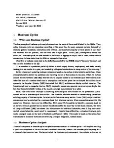
less and investment growth is somewhat more. Hours, on the other hand, exhibit no growth at all and actually fall by about 0.1 percent per year. Standard deviations provide information on the relative volatility of the different series. Investment growth is the most volatile followed by output, hours, wages and consumption respectively. Autocorrelations measure the amount of persistence of the series from one year to the next. For example, the correlation coefficient between the growth in consumption in one year is about .4 with the previous year's growth in consumption. Only real wages and consumption show much evidence of persistence in growth rates. Finally, all the series are highly correlated with output and thus are procyclical. The lowest correlation with output is exhibited by real wage growth with a correlation coefficient of .59 and the highest is investment with a correlation coefficient of .92. Productivity Shifts In order to see more quantitatively the sorts of real economic fluctuations generated by the simple model economy it is necessary to obtain some measure of the productivity shocks. A crude but straightforward method is to follow the example provided by Solow to construct a measure of the state of productivity. Using the data described above and the gross stock of real nonresidential fixed private capital, a Solow technology series is readily constructed."6 The annual percentage rate of change 6All data are taken from the CITIBASE data service except the capital stock, which is taken from the August 1986 issue of the Surveyof Current Business.An estimate of labor's share of output is also required (see footnote 12).
UnderstandingReal Business Cycles
63
Figure 1
Annual Growth Rate of Technology 6 ~D 4 2 0
,
'
-2 >
-4 -6 1955
1960
1965
1970
1975
1980
1985
in technology is plotted in Figure 1. The picture corresponds to most observers' impressions that productivity growth was on average higher in the 1960s than the 1970s and 1980s. The growth rate of this 32 year period averages 0.8 percent per year and has a standard deviation of about 1.9 percent. The maximum growth rate is about 4.0 percent and the minimum is about -3.5 percent. There is only slight evidence of serial correlation in these growth rates so to a first approximation it seems acceptable to view the level of productivity as a random walk. These computed productivity disturbances may or may not be very good estimates of the true changes in productivity. However, the real business cycle model delivers explicit and tight restrictions on the behavior of consumption, hours worked, investment, and thus output, conditioned on the disturbances to the model being of a technological source. If the measured technological shocks are poor estimates (that is, if they are confounded by other factors such as "demand" shocks, preference shocks or change in government policies, and so on) then feeding these values into our real business cycle model should result in poor predictions for the behavior of consumption, investment, hours worked, wages and output. Real Business Cycles Given the form of preferences and technology, the model is used to obtain the responses of the simple neoclassical model to observed productivity shifts.'7 These results are summarized in Panel B of Table 1. The model produces sample means that are very close to the data for output, consumption and hours, but is too low for investment and too high for wages. The model generates the same volatility rankings 17The responses are computed using the stochastic version of the model that assumes productivity shifts are known to follow a random walk. Future value of the shifts are not known to the agents in the economy but they form rational expectations of these shifts based on their known stochastic structure.
64
Journalof EconomicPerspectives
Figure2 Annual Growth Rate of Real Output ~~~)
cl cl
6
-~~~~~~ ~ACTUAL
0
-2 -4 -6 ,
,
I
_
1960
1955
I ,
,I .,,, , I
,
1965
,.| I
, ,,I
,
,
1970
I
1975
,
, ,I , ,
1980
1985
for Y, C, I, but the absolute standard deviation of investment is slightly lower and that for consumption is slightly higher than in the actual data. The major discrepancy appears to be that in the model the growth rate of hours has a standard deviation that is less than one-half of that in the data. In terms of serial correlation properties, the model generates slightly, but perhaps not significantly, more positive autocorrelation than seems present in the data. Perhaps the numbers of most interest in the table are those in the last column of Panel B. These are the correlation coefficients of the predicted outcomes with the
Figure3 Annual Growth Rate of Real Consumption 6 ACTUAL 4
- .
'
-
,
PREDICTED
2' 0
0
X
-4 -6 I
5I
1955
1960
I
1965
I
,
1970
I
,
1975
19I
1985
1980
1985
CharlesI. Plosser 65
Figure4 Annual Growth Rate of Real Investment u
ACTUAL
10
~
ct
~ ~
~
~
~
~
~
~
--
PREDICTED
5 r. bIo
a
a~
.\1
|v
tf
X
0_
-5
-10
1955
1960
1965
1970
1975
1985
1980
actual series and range from .52 for wages to .87 for output. To many economists, the whole idea that such a simple model with no government, no money, no market failures of any kind, rational expectations, no adjustment costs and identical agents could replicate actual experience this well is very surprising. This is especially true given that most macroeconomic research over the past 50 years stressed the importance of one or more of the above factors in explaining business fluctuations. Figures 2 through 6 provide a visual impression of these correlationsby plotting both the actual and predicted growth rates of each of the five variables. As expected from the evidence presented in Table 1, the growth rate of hours worked exhibits the
Figure5 Annual Growth Rate of Hours Worked 6 ACTUAL ----
4
~ 0
PREDICTED
2 0
'
-',i-
4.
-4 -6 1955
1960
1965
1970
1975
1980
1985
66
Journalof EconomicPerspectives
Figure6 Annual Growth Rate of Real Wage Rate 6 -ACITUAL
0
-2 Q
-4
,6 1
1955
1
t
i
I
1960
I
I
I
,. I
1965
I
I
I
I
I
1970
I
I
I
I
t
1975
I
I
l. I
I
1980
I
I
I,
1985
biggest discrepancy between actual and predicted. Nevertheless, the simple model appears to replicate a significant portion of the behavior of the economy during recessions as well as other periods.
Government Policies and Suboptimal Equilibrium Two key features of the real business cycle model discussed so far are that business cycles are initiated by shocks to technology and that fluctuations are Pareto optimal. Neither of these conditions, however, are necessary features of the real business cycle approach. Many economists, for example, argue that government tax and spending policies are an important source of real disturbances to the economic system. The incorporation of government into the real business cycle models makes it possible to address important questions regarding changes in fiscal policies in the presence of distortionary taxes. Of particular interest is the case where the tax and spending policies are functions of the state of the economy. Variation in government spending introduces a potential source of demand disturbances to the model. The presence of distortionary taxes generally breaks the link between Robinson Crusoe's optimal decisions and Pareto efficiency, since removing the distortions will usually raise welfare. Nevertheless, competitive equilibria can be computed and analyzed that are not Pareto optimal but suboptimal equilibria. The theoretical underpinning of this line of research draws from earlier work by Arrow (1962), Hall (1971) and Brock (1975) and a more recent series of papers by Romer (1983, 1986, 1987). The basic line of reasoning is that in an economy with many agents, each can take the government'sspending and taxing policies as given in their choice problem. The only additional restrictionis that aggregate behavior satisfy
RealBusinessCycles 67 Understanding
the government's budget constraint. These models provide an artificial laboratory for answering questions regarding policy changes that is not subject to the criticism of Lucas (1976). The intuition underlying the effects of unproductive (as assumed in most Keynesian analyses) government purchases in the neoclassical model is basically found in Barro (1981) and Hall (1980).18 These authors emphasize two sorts of influences. First, raising government purchases induces a negative wealth effect that acts to reduce consumption and raise work effort and output. Second, raising government purchases also induces intertemporalsubstitution when the increase is temporary. This results in lower consumption, lower investment, higher work effort and higher output. The relative importance of the wealth and intertemporal substitution channels remains unresolved. Barro and Hall assume that the intertemporal substitution channel is quantitatively more important so that temporary changes in government purchases are more important than the wealth channel. Baxter and King (1988) have investigated these effects within a real business cycle model and have concluded that for plausible values of the parameters more persistent changes in government purchases have larger output "multipliers" than more temporary changes in purchases. Temporary purchases on the other hand, have a more negative impact on investment than more persistent purchases.19 The implications of distortionary taxation within the neoclassical model have been a topic in public finance for some time. What distinguishes the recent work from the earlier efforts, including Hall (1971) and more recent analyses by Abel and Blanchard (1983) and Judd (1985) is that tax rates are assumed to be functions of the state of the economy. King, Plosser and Rebelo (1988b) summarize the implications of a real business cycle model under a period-by-period balanced budget, where tax revenue is based on an output tax and government spending is rebated as lump-sum transfers. In this case a positive productivity shift requires a decline in the tax rate in order to maintain budget balance. This reduction in tax rates reinforces the efforts of the productivity shock on after-tax labor productivity and further increases work effort in response to technology shocks. Thus work effort (and investment, for analogous reasons) are more volatile in this economy.
The Real Business Cycle Research Agenda The results in the previous sections indicate that the basic neoclassical model of capital accumulation can provide an important framework for developing our understanding of economic fluctuations. The models investigated to date, however, are not entirely satisfactory. Indeed, it would be extraordinary if they were. The real business I1n this discussion government purchases are assumed to be financed by lump-sum taxes or reductions in transfer payments. In this case increase in government purchases can be viewed as negative shocks to production that enter additively. See Abel and Blanchard (1983). 1 Another quantitative example can be found in Wynne (1988), who uses a real business cycle model that includes government purchases to account for the behavior of the U.S. economy during World War II.
68
Journal of EconomicPerspectives
cycle research program is to pursue this class of models to determine how far the approach can take us. In this section, I highlight some of the issues that are likely to be important for developing and evaluating this important class of models.
Multi-Sector Extensions The basic neoclassical model has been explored along various dimensions in an effort to expand the scope of the method of analysis. Long and Plosser (1983) explore a model with multiple sectors in order to understand the comovement across sectors in response to shocks that are potentially sector specific. Their interest in multiple sectors is motivated by the observation that many sectors of the economy tend to move together but some sectors lead while other sectors lag the general state of business activity. Multi-sector models are the only way to address this phenomenon and understand it since one-sector models proceed by assuming that the answer is the existence of aggregate or common shocks.20 Black (1987) argues that multi-sector models are important, particularly if unemployment is to be explained. Black bases his argument on the notion that both human and physical capital is highly specialized. Shocks to either preferences or technologies will generally require resourcesin the form of labor and capital to move between sectors. Since these inputs are specialized, it will be costly to make this adjustment. As a result, unemployment can be expected to rise above its long-run level.
Labor Markets A major thrust of much recent research in the real business cycle area is to expand and extend the basic model in ways that would result in a better match of the model's predictions for hours and actual hours worked. The source of conflict is that the logarithmic preferences adopted for the purpose of the earlier estimates imply a labor supply elasticity that is much higher than the estimates obtained by labor economists using panel data on prime age males. Thus, the model appears to be incapable of generating sufficient volatility in hours without being in conflict with evidence from detailed microeconomic investigations. This view, however, is unduly pessimistic. Numerous approaches have been pursued (though none has been completely satisfactory to date) that attempt to modify the model in ways that make it compatible with the microeconomic evidence. One approach pursued by Kydland and Prescott (1982) stresses the importance of preference structures that are not time separable. In their formulation, the current utility of leisure depends on past leisure in an explicit way. This has the effect of permitting an increase in the intertemporal substitutability of leisure which in turn makes hours worked more volatile.
20
Baxter (1988) presents a quantitative analysis of a two sector model in the context of an international real trade model.
CharlesI. Plosser
69
Rogerson (1988) and Hansen (1985) explore the consequences of indivisibilities in the labor supply decision that require agents to work either full-time or not at all. This is in contrast to the simple model where agents are permitted to vary hours worked continuously. The result is that the volatility of hours worked in response to productivity shifts is significantly increased while estimated labor supply elasticities would remain low for working males. Another approach to enhancing the response hours worked in the model is to allow for heterogeneity across agents in the economy. Examples of this approach are found in Cho and Rogerson (1988), Kydland (1984), King, Plosser and Rebelo (1988b) and Rebelo (1987). All of these papers suggest that there can be important downward biases in estimates of aggregate labor supply elasticity when there are agents with different skill levels.
Endogenous Growth Another important area for research focuses on the role played by the technology shocks. Solow's view of technological change included anything that shifted the production function other than measurable capital or labor. As an empirical proposition, Solow's results indicate that such shifts, if viewed as exogenous, account for a substantial portion of economic growth. The real business cycle model stresses that these shifts play an important role in economic fluctuations as well. This is not entirely satisfactory. It would be useful if we had a better understanding of the economics of growth that did not rely as heavily on such an exogenous unobservable process. Work by Uzawa (1965), Romer (1986) and Lucas (1988) modifies the basic neoclassical model to permit growth to be an endogenous outcome of the technology. The key to obtaining such a result is eliminating the diminishing returns in the production process. King and Rebelo (1986, 1988) provide examples of this strategy and explore its implications for economic fluctuations and certain types of fiscal policies. The idea is to permit human capital (labor-augmenting technical change) to be produced using physical capital and human capital as inputs to a constant returns technology. The results are interesting and potentially important. For example, purely temporary productivity shifts can have permanent effects on the level of economic activity. The reason is that a change in productivity that results in more output will generally result in some increased resources being allocated to the production of additional human capital. Thus allocation decisions affect the level of technology and the growth in the economy. These models have the additional implication that such variables as output, consumption and investment are integrated or possess a stochastic trend. This result is appealing because as noted above, Nelson and Plosser (1982) have argued that many economic time series appear to possess stochastic trends or random walk components. Finally, productivity shocks in these models can initiate complex patterns of adjustment to a new growth path. These transition paths generally include complex changes in work effort, investment and consumption. An understanding of these models is likely to be an important part of understanding economic fluctuations, as well as economic development, while reinforcing the concept that growth and fluctuations are intimately connected.
70
Journalof EconomicPerspectives
Money Real business cycle research has focused almost exclusively on models with no role for money. For some economists, this not only doesn't represent progress, but borders on blasphemy. My view, and that of many other real business cycle researchers, is that the role of money in an equilibrium theory of growth and fluctuations is not well understood and thus remains an open issue. Some researchers, including King and Plosser (1984), Kydland (1987), Eichenbaum and Singleton (1986) and Cooley and Hansen (1988), have explored methods of incorporating money and investigating its implications in a real business cycle model. Unfortunately there is little agreement on what constitutes the most fruitful approach at this time. Nevertheless, without an understanding of the real fluctuations inherent in the basic neoclassical model without money it will be difficult if not impossible to measure the quantitative importance of money in actual business fluctuations. The nature and magnitude, however, of the fluctuations and responses in the real neoclassical model means that real business research poses a challenge to conventional views regarding the relative importance of money. This is particularly true given the difficulties economists have faced in developing a convincing and coherent explanation of the monetary transmission mechanism.
Strategies for Estimation and Hypothesis Testing A final part of the research agenda relates to empirical assessments of the real business cycle approach. The approach adopted to date takes as given the technological shocks and asks how other variables-such as consumption, work effort and investment-respond over time to these impulses. It would be useful to obtain an independent measure of these shocks or identify observable variables that could proxy for them. Expanding the models to include government, endogenous growth or international trade are important steps in this process. A closely related topic, and one of intense debate among researchers, is the strategy used to investigate the implications of the model. The traditional way of estimating and testing an economic model is to write down a set of structural equations, estimate the parameters and test any restrictions not necessary to identify parameters. In the context of the real business cycle models described earlier this strategy corresponds to obtaining Robinson Crusoe's optimal decision rules for consumption, work effort and investment,jointly estimating the parameters of technology and preferences and then testing the overidentifying restrictions imposed on these decision rules.21
An alternative strategy has been pursued in much of the real business cycle literature. The technique, made popular in this literature by Kydland and Prescott (1982) (but more widely employed in the applied general equilibrium literature like Ballard, Shoven and Whalley, 1985), is called "calibration." The strategy is to choose values for certain key parametersof the underlying preferencesand technologies using 21See, for example, Altug (1985) and Christiano (1988).
RealBusinessCycles 71 Understanding
evidence from other empirical studies. This restrictsthe number of free parameters in the model. Using these parameter values, the stochastic properties (means, variances, autocorrelations and cross-correlations)of certain key variables are constructed. The remaining free parameters are chosen to yield, as close as possible, a correspondence between the moments predicted by the model and those in the sample data. A formal definition of what constitutes a good fit or the metric along which fit should be judged is not explicitly offered by Kydland and Prescott.22 The appropriate empirical strategy for investigating the class of models discussed in this paper remains an open area of research. Ultimately, this issue must be addressed and real business cycle models will have to face and pass more stringent empirical tests than they have to date.
Conclusions The basic framework of real business cycle analysis is the neoclassical model of capital accumulation. This is the natural starting point to begin the study of dynamic fluctuations. While frequently interpreted as a model of economic growth, the neoclassical model generates fluctuations in response to external disturbances that resemble business cycles. While real technology shocks have occupied the central focus in the literature, other shocks arising from preferences, government, terms of trade and eventually money can be included. Thus real business cycle models do not have to be confined to analyzing only technological or productivity shocks. Nevertheless, these real technological disturbances generate rich and neglected dynamics in the basic neoclassical model that appear to account for a substantial portion of observed fluctuations. Real business cycle theory is still in its infancy and thus remains an incomplete theory of the business cycle. Yet the progress to date has had a significant impact on research in macroeconomics. In particular, simple real business cycle models have demonstrated that equilibrium models are not necessarily inconsistent with many characteristics attributed to the business cycle. In so doing these models have changed the standard by which macroeconomic theories are judged and provided the foundations for an understanding of business cycles that is based on the powerful choice theoretic analysis that is at the core of economic reasoning. The appeal of this line of research is the apparent power of some very simple economic principles to generate dynamic behavior that was heretofore thought to be incompatible with any notion of equilibrium. While the promise is great, much work remains before economists have a real understanding of business cycles.
22
The traditional econometric approach and calibration are not mutually exclusive, however. Singleton (1988) discusses how the calibration approach of Kydland and Prescott might be formulated in the context of the generalized method of moments procedure proposed by Hansen (1982).
72
Journalof EconomicPerspectives
Appendix Specifying a Model of Real Business Cycles This appendix presents a more analytical summary of the basic neoclassical model discussed in the second section of the paper. The first step is to specify the economic environment by describing the preferences, technology and endowments of the model economy. The Neoclassical Model Preferences. The economy is assumed to be populated by many identical agents (households) that live forever.23The agent's utility at time t is assumed to be of the form U- = YLxo/3usu(C,ts, L,?s), where C, is the level of consumption of the single produced good and L, is the amount of leisure consumed. The utility discount factor is assumed to be constant. Leisure is included because variation in work effort is an important feature of short-runfluctuations and yet is frequently absent from otherwise similar models encountered in the growth literature. The momentary utility function u(-) is assumed to be concave and twice continuously differentiable. Production. The single final good, Y,, is produced by a constant returns to scale production technology given by Y, = F,F(Kt, N,), where K, is the predetermined capital stock (chosen at t - 1) and Al is labor input in period t. 0, is a temporary shift factor that alters total factor productivity. The produced commodity Y can either be consumed or invested. The production function is also assumed to be concave and twice continuously differentiable. CapitalAccumulation.The invested commodity becomes part of the capital stock that is available on input to production next period. I'his capital stock evolves as K, ? = (1 -6) K, + I, where I, is gross investment and 8 is the depreciation rate of capital. ResourceConstraints. Agents also face resource constraints in each period on the use of the commodity and time. These constraints are L, + N, < 1 and C, + I, < Y, where the time endowment is normalized to unity. These are nonnegativity constraints Li, C,, N, and K, as well. The computation of the competitive equilibrium prices and quantities that are implied by this framework is simplified by recognizing that all individuals are alike. Thus, it is easy to imagine a representative agent, Robinson Crusoe, and determine how his optimal choice of consumption, work effort and investment evolve over time. Debreu (1954) and Prescott and Lucas (1972) have shown that we can interpret the utility maximizing choices of consumption, investment and work effort by Robinson Crusoe as the per capita outcomes of a competitive market economy. Robinson Crusoe's choice problem is to maximize his lifetinme(infinite) utility subject to a sequence of resource constraints. The Lagrangian associated with the 23The use of an infinitely-lived agent can also be interpreted as an finite-lived agtnt with an operative
bequest motive that links the current generation's utility with future generations. See Barro (1974) or Miller and Upton (1974).
CharlesI. Plosser 73
maximization problem is Y=
L 13'[u(C,, =1)
1 - N)] + E Xi[tF(K,,
N)
C, - Kt+I + (1 -8)Kt]
-
t=()
- N is substituted for L, I Kt Iis substituted for It, &JF(Kt, N,) (1 - 8)K, is substituted for Yt, and X, is the Lagrange multiplier associated with the period t resource constraint Y, - Ct - It = 0. The first-orderefficiency conditions for this problem are obtained by differentiating Y with respect to the variables of choice at each time t, C,, Nt, Kt/I and the multiplier, which yields
where 1
-
U1(Ct, I
u2(C`, 1-
Nt)-
XttF2(K,,
Nt+1) + (1
IX,-tI[Ot+IFI(K,?I,
OEtF(Kt, At) + (1
-
N)-X
6)Kt
-
At)
=
0
=
0
-x,
= 0
Kt+1 -C
= O
8)]
which must hold for all t = 1, 2, ... oo. F () and u1(-) denote the partial derivatives of F and u with respect to the ith argument. In addition, it is common to assume that the transversality condition, limt_
tX t Kt + 1
=
0, is satisfied.
Given specific functional forms for u(-) and F(-) the solution to this maximum problem is the time paths of the four unknown choice variables, C, N, K and X that satisfy these efficiency conditions for some initial condition Ko and a sequence of productivity disturbances {tQ}x%0.24 These time paths can be expressed in the form of time invariant decision rules that take the form Ct =
C(K,,
Nt =N(Ktj
- ) t 4i-s
Ktj= K(Kt,t{+s
'
I So+O)8
}2=o)'
The competitive market prices implied by these optimal quantities are a real interest rate between t and t + 1, rt, and a real wage rate, w,. These are readily determined to be (1 + r,) = X,1(X,?+1,)and w, = (Ot)F)(Kt,N,) and are the ones that would prevail in the spot market for labor services and a one-period sequential loan market.25Another important feature of this economy is that in the absence of changes 24If these disturbances
are ktnown, the equilibrium prices and quantities are a perfect foresight equilibrium. If {0, } is a stochastic process, Robinson Crusoe forms expectations about the future values using all currently available information. In this case the equilibrium is a rational expectations equilibrium. 25''lhis is but one of the mnarket structures that would support the optimal allocations as a competitive equilibrium. An alternative nmarket structure in the labor market might be that agents are paid a wage rate that corresponids to the annuitized rate based on the present value of their entire future stream of marginal products.
74
Journal of EconomicPerspectives
in technology (i.e. E),= 0, for all t), and given some initial capital stock, per capita values of consumption, hours, capital and output, converge to constants, referred to as the steady state. Approximate Solutions Under most specifications of preferences and production functions, the four first-order conditions given earlier constitute a set of nonlinear difference equations. Thus it is usually impossible to solve this maximum problem analytically for the optimal decisions rules of Robinson Crusoe. Consequently, real business cycle researchers find it necessary to compute approximate solutions to Robinson Crusoe's choice problem. These approximation procedurestypically result in decision rules that are linear K, and the e's. The details of various procedures available to compute these approximately optimal quantities and competitive prices are beyond the scope of this essay. Nevertheless, the basic idea pursued in King, Plosser and Rebelo (1988a) is intuitively straightforwardand is the method employed in the text.26 The first step in the approximation procedure is to choose a point to approximate around. The natural choice is the stationary point or steady state, denoted [Cs, K5, Ns, Xs]. The second step is to express the four first-orderconditions in terms of the percentage deviations from the stationary values (defined as C, K, N, etc.) and then take a linear approximation to each condition. This results in a set of linear difference equations in percentage deviations from the steady state. Solving this linear system produces the approximately optimal decision rules that correspond to the three time-invariant decision rules.27These decision rules are linear functions of the predetermined capital stock and the sequence of productivity shifts. For example, efficient capital accumulation can be written as
K1+1
=
,1IK1 + '101
+
I2
E j-O
2
+j+ 1
where 1, 2' %1and I2 are complicated functions of the underlying parameters of tastes and technology. Thus next period's capital stock depends on the current capital stock, the current level of productivity 0, and the entire future path of shifts discounted by 2. The conditions on the problem pretty much guarantee that I < 1 and P2 > 1. The (approximately) optimal decision rules for C1 and NAtake similar forms.28 26For an alternative strategy, see Kydland and Prescott (1982). 27Solving this system also requires imposing the transversality condition. See King, Plosser and Rebelo (1988a) for more details of this solution technique. Several authors including Christiano (1982) and Rebelo and Rouwenhorst (1989) have studied the accuracy of these linear approximations. 28Generalizing this approach to handle the case of stochastic variation in productivity is not difficult. TIhe method of certainty equivalence amounts to positing a specific stochastic structure for the (3's and substituting their conditional expectations for the future values.
RealBusinessCycles 75 Understanding
An Example Economy In the text a specific example economy is used to quantitatively measure the responses of a real business cycle model to estimated productivity shifts. As indicated in the text preferences are taken to be logarithmic such that u(C,, L,) = log(C1) + NL log(L,). The production technology is taken to be Cobb-Douglas Y, = ,K `-aN,a, or, expressing the technology shift 0, as labor-augmenting Y, = K,- a(el/`N )'. The technology shifts are computed following Solow and are assumed to follow a logarithmic random walk for purposes of computing the approximate optimal decisions. The remaining parametersare chosen assuming the time interval is one year and correspond to those used in King, Plosser and Rebelo (1988a,b). Labor's share (a = .58) is computed as the average ratio of total employee compensation to GNP for the period 1948-1985. Depreciation (S = .10) is simply assumed to be 10 percent per annum. The utility discount factor (/B = .95) is chosen to yield a return to capital of 6.5 percent per annum, which is the average real return to equity from 1948-1981. Finally, the utility parameter XL is chosen indirectly by specifying that steady state hours work is .20 which is based on the average fraction of hours devoted to market work during the 1948-1985 period. andsuggestions m The authorhas benefited fromthecomments of MarianneBaxter,FischerBlack, Karl Brunner,ThomasCooley,RobertKing, SergioRebelo,Carl Shapiro,Joseph Stiglitz and TimothyTaylor. The BradleyPolicy ResearchCenterat the W.E. SimonGraduateSchoolof BusinessAdministration providedfinancial support.
References Abel, Andrew B., and Oliver J. Blanchard, "An Intertemporal Model of Savings and Investment," Econometrica, May 1983, 51, 675-692. Altug, S., "Gestation Lags and the Business Cycle: An Empirical Investigation," unpublished manuscript, University of Minnesota, 1985. Arrow, Kenneth, "The Economic Implications of Learning by Doing," Reviewof EconomicStudies, June 1962, 29, 155-173. Ballard, Charles L., John B. Shoven, and John Whalley, "General Equilibrium Computations on the Marginal Welfare Costs of Taxes in the United States," AmericanEconomicReview, March 1985, 75, 128-138. Barro, Robert J., "Are Government Bonds Net Wealth?" Journal of PoliticalEconomy,NovemberDecember 1974, 82, 1095-1117. Barro, Robert J., "Output Effects of Govern-
ment Purchases," Journal of Political Economy, December 1981, 89, 1086-1125. New York: Barro, Robert J., Macroeconomics, John Wiley & Sons, 1987. Baxter, Marianne, "Dynamic Real Trad Model: New Directions for Open Economi Macroeconomics," Rochester Center for Eco nomic Research, University of Rochester, WI #167, 1988. Baxter, Marianne, and Robert G. King, " Mul tipliers in Equilibrium Business Cycle Models,' unpublished manuscript, University of Rochester 1988. Black, F., BusinessCyclesand Equilibrium.NeN York: Basil Blackwell, 1987. Brock, William A., "A Simple Perfect Foresig, Monetary Model," Jourmalof MonetaryEconomic! April 1975, 1, 133-150.
76
Journalof EconomicPerspectives
Brock, William A., and Leonard J. Mirman, "Optimal Economic Growth and Uncertainty: The Discounted Case," Journalof EconomicTheory, June 1972, 4, 479-513. Campbell, John, and N. Gregory Mankiw, "Are Output Fluctuations Transitory?" Quarterly Journalof Economics,1987, 102, 857-880. Cass, David, "Optimum Growth in an Aggregative Model of Capital Accumulation," Econometrrica, July 1965, 32, 223-240. Cho, F., and Richard D. Rogerson, "Family Labor Supply and Aggregate Fluctuations,"Journal of MonetaryEconomics,1988, 21, 233-245. Christiano, L., "Why Does Inventory Investment Fluctuate So Much?" Journal of Monetary Economics, 1988, 21, 247-280. Christiano, L., "Solving a Particular Growth Model by Linear Approximation and by Value Function Iteration," Federal Reserve Bank of Minnesota, Discussion Papers #9, 1989. Cooley, Thomas F., and G. Hansen, "The Inflation Tax and the Business Cycle," Rochester Center for Economic Research, University of Rochester, WP #155, 1988. Debreu, Gerard, "Valuation Equilibrium and Pareto Optimum," Proceedingsof the National Academyof Sciencesof the U.S., 1954, 38, 886-893. Eichenbaum, Martin, and Kenneth J. Singleton, "Do Equilibrium Business Cycle Theories Explain Post-war Business Cycles?." In Fischer, S., ed., NBER Macroeconomics Annual, 1986, 91- 134. Friedman, Milton, "The Role of Monetary Policy,' AmericanEconomicReview,March 1968, 58, 1- 17. Greenwood, J., Z. Hercowitz, and Gregory W. Huffman, "Investment, Capacity Utilization and the Real Business Cycle," AmericanEconommic Review,June 1988, 78, 402-17. Hall, Robert E., "The Dynamic Effects of Fiscal Policy in an Economy with Foresight," Review of EconomicStudies,April 1971, 38, 229-244. Hall, Robert E., " Labor Supply and Aggregate Fluctuations." In Carnegie-Rochester Serieson Public Policy, 12, Amsterdam: North Holland, 1980. Hansen, G., "Indivisible Labor and the Business Cycle," journal of MonetaryEconomics,1985, 16, 309-327. Hansen, Lars, " Large Sample Properties of Generalized Method of Moment Estimators," Econometrica, July 1982, 50, 1029-1054. Hicks, John, " Equilibrium and the Cycle," reprinted in Hicks, John, CollectedEssay on Economic Theory, Vol. II, Money, Interestand Wages. Oxford: Basil Blackwell Ltd., 1933. Hicks, John, Valueand Capital.London: Oxford University Press, 1939. Hicks, John, Capital and Growth.New York:
Oxford University Press, 1965. Judd, Kenneth, "Short Run Analysis of Fiscal Policy in a Simple Perfect Foresight Model," Journal of PoliticalEconomy,April 1985, 93, 298-319. King, Robert G., and Charles Plosser, "Money, Credit and Prices in a Real Business Cycle," AmericanEconomic Review,June 1984, 74, 363-380. King, Robert G., Charles Plosser, and Sergio Rebelo, "Production, Growth and Business Cycles I. The Basic Neoclassical Model," Journalof MonetaryEconomlcs,1988a, 21, 195-232. King, Robert G., Charles Plosser, and Sergio Rebelo, "Production, Growth and Business Cycles II. New Directions," Journalof MonetaryEconomics, 1988b, 21, 309-341. King, Robert G., Charles Plosser, James Stock, and Mark Watson, "Stochastic Trends and Economic Fluctuations," Rochester Center for Economic Research, working paper X79, 1987. King, Robert G., and Sergio Rebelo, "Business Cycles with Endogenous Growth," unpublished manuscript, University of Rochester, 1986. King, Robert G., and Sergio Rebelo, "Public Policy and Economic Growth," unpublished working paper, University of Rochester, 1988. Koopmans, T., "On the Concept of Optimal Growth." In TheEconometric Approachto Development Planning.Chicago: Rand McNally, 1965. Kydland, Finn E., "Labor Force Heterogeneity and the Business Cycle," in Carnegie-Rochester ConferenceSerieson PublicPolicy, 1984, 21, 173-208. Kydland, Finn E., "Ihe Role of Money in a Real Business Cycle Model," unpublished manuscript, Carnegie-Mellon University, 1987. Kydland, Finn E., and Edward C. Prescott, "Time to Build and Aggregate Fluctuations," Econometrica,November 1982, 50, 1345-1370. Long, John B., and Charles Plosser, "Real Business Cycles," Journal of Politzcal Economy, February 1983, 91, 1345-1370. Long, John B., and Charles Plosser, "Sectoral vs. Aggregate Shocks in the Business Cycle," AmericanEconomicReview,1987, 77, 333-337. Lucas, Robert E., "Econometric Policy Evaluation: A Critique." In Carnegie-Rochester Conference Serieson PublicPolicy, 1976, 1, 19-46. Lucas, Robert E., "Understanding Business Serieson PublicPolicy, Cycles." In Carnegie-Rochester 1977, 5, 7-29. Lucas, Robert E., "Methods and Problems in Business Cycle Theory," Journal of Money, Credit and Banking,November 1980, 12, 696- 715. Lucas, Robert E., ' On the Mechanics of Economic Development," Journal of MonetaryEconomics, 1988, 22, 3-42. Miller, Merton H., and Charles W. Upton, Macroeconomics: A NeoclassicalIntroduction.Homewood, Illinois: Irwin, 1974.
CharlesI. Plosser 77
Mitchell, W., BusinessCycles:TheProblemandIts Setting.New York: National Bureau of Economic Research, 1927. Muth, Richard F., "Rational Expectations and the Theory of Price Movements," Econometrica, 1961, 29, 315-335. Nelson, Charles R., and H. Kang, "Spurious Periodicity in Inappropiately Detrended Time Series," Econometrica, 1981, 49, 741-751. Nelson, Charles R., and Charles Plosser, "Trends and Random Walks in Macroeconomic Time Series: Some Evidence and Implications," Journalof MonetaryEconomics,September 1982, 10, 139-167. Phelps, Edmund S., GoldenRules of Economic Growth.New York: Norton, 1966. Prescott, Edward C., "Theory Ahead of BusiSeness Cycle Measurement." In Carnegie-Rochester ries on PublicPolicy, 1986, 25, 11-66. Prescott, Edward C., and Robert E. Lucas, "A Note on Price Systems in Infinite Dimensional EconomicsReview,June 1972, Space," International 13, 416-422. Rebelo, Sergio, "Tractable Heterogeneity and Near Steady State Dynamics," unpublished manuscript, University of Rochester, 1987. Rebelo, Sergio, and G. Rouwenhorst, "Linear Quadratic Approximations Versus Discrete State Space Methods: A Numerical Evaluation," unpublished working paper, University of Rochester, 1989. Rogerson, Richard D., "Indivisible Labor, Lotteries and Equilibrium," Journalof MonetaryEconomics,1988, 21, 3-16. Romer, Paul, "Dynamic Competitive Equilibria with Externalities, Increasing Returns and Unbounded Growth," doctoral dissertation, University of Chicago, 1983. Romer, Paul, "Increasing Returns and Long Run Growth," Journal of PoliticalEconomy,1986,
94, 1002-1073. Romer, Paul, "Increasing Returns, Specialization, and External Economies: Growth as described by Allyn Young," Rochester Center for Economic Research, working paper #19, 1987. Singleton, Kenneth, J., "Econometric Issues in the Analysis of Equilibrium Business Cycle Models," Journal of MonetaryEconomics,1988, 21, 361-386. Slutsky, E., "The Summation of Random Causes as the Source of Cyclical Processes,"Econometrica,1937, 5, 105-146. Solow, Robert, "A Contribution to the Theory of Economic Growth," Quarterly Journal of Economics,February 1956, 70, 65-94. Solow, Robert, "Technical Change and the Aggregate Production Function," Review of EconomicStudies,August 1957, 39, 312-320. Stock, James H., and Mark H. Watson, " Variable Trends in Economic Time Series,"Journalof Economic Perspectives, Summer 1988, 2, 147-174. Surveyof CurrentBusiness,United States Department of Commerce/Bureau of Economic Analysis, August 1986. Swan, T., "On Golden Ages and Production Functions." In D. Berril, ed., Economic Development with Special Referencesto SoutheastAsia, London: Macmillan, 1963. Uzawa, Hirofumi, "Optimal Technical Change in An Aggregative Model of Economic Growth," InternationalEconomicReview, January 1965, 6, 18-31. Uzawa, Hirofumi, "Neutral Inventions and the Stability of Growth Equilibrium," Reviewof EconomicStudies, February 1961, 28, 118-124. von Hayek, Friederich August, Pricesand Production.London: George Routledge & Sons, 1932. Wynne, Mark A., "The Aggregate Effects of Temporary Government Purchases,"unpublished manuscript, University of Rochester, 1988.