Urban Crime and Residential Decisions: Evidence from Chicago Anthony E. Tokman* This Version: November 2017

Abstract Rising crime rates in many U.S. cities from the 1950s to the 1990s were at least partly responsible for the large-scale outmigration of urban residents to the suburbs, especially in the Northeast and Midwest. While subsequent declines in crime have allowed some cities to reverse the outflow, several major cities still face a high incidence of violent and property crime. In this paper I apply a discrete choice gravity model to measure the impact of crime on residential and commuting decisions in the city of Chicago. I find that a 10% localized increase in the violent crime rate is associated with a roughly 1.1% decline in residential amenity, which translates into a 1.9% population decline at a given location. City-wide, a 10% increase in the crime rate may decrease population by between 0.7 and 2.8%, depending on where the crime is concentrated. I also estimate the effect of large-scale crime reductions on the city’s troubled West Side.

1

Introduction

Cities have long brought tremendous benefits to their residents by providing easier access to markets, facilitating information exchange and learning, and encouraging socialization and the growth of communities. Cities also benefit non-residents by stimulating innovations—both technological and cultural—that find their way well beyond city borders.1 The rate of urbanization rapidly increased in the 19th century with the arrival of the industrial revolution. Today, roughly 80% of Americans live in cities, up from 40% in 1900 and a mere 5% when the first census was taken in 1790 (U.S. Census 2012).2 This percentage is similar throughout most of Europe and in much of the developed world, and the rate of urbanization is especially high today in many developing countries. Despite cities’ many attractive qualities, however, city life brings a number of drawbacks: land is scarcer and therefore more expensive in cities than in rural areas; cities have historically suffered from high levels of air and water pollution, and many still do; and cities typically have higher *

Federal Reserve Bank of Chicago; email: [email protected]. The views expressed herein do not reflect those of the Federal Reserve Bank of Chicago or the Federal Reserve System. 1 See, e.g., Jacobs (1969), Glaeser et al. (1992), and Glaeser (1999). 2 The U.S. Census defines a city as any populated area with a population of over 2,500, which is a rather generous definition. Perhaps the more relevant statistic is that 55% of Americans live in metropolitan areas with populations of over one million—truer “cities” in the colloquial sense.

1

crime rates than rural areas, which has especially been true in the United States over the last sixty years. While crime generally doesn’t prevent people from living in America’s metropolises, it does affect where they choose to live within these metropolises; crime is one factor that has pushed many, typically wealthier, residents to the suburbs in the process called “urban flight.” While this trend has been partly reversed in many cities over the last 20 years, crime still plays an important role in keeping residents (especially the middle and upper classes) out of certain neighborhoods. And it remains an unfortunate part of the lives of many people who cannot afford moving to safer neighborhoods. In this paper I measure the impact of violent and property crime on residential choices in Chicago, although the model I employ is general enough to handle any metropolitan area, given sufficient data. The U.S.’s third-largest city, Chicago, like many other Northeastern and Midwestern cities, experienced significant urban flight between the 1950s and 1990s. While the causes of this urban flight were many, it is no accident that it accompanied a four-fold rise in the homicide rate, from 8 per 100,000 residents in 1950 to 33 per 100,000 residents in 1990 (Newberry Library 2004). Despite seeing a small rise in the 1990s, Chicago’s population again declined in the 2000s. And although Chicago’s violent crime has fallen significantly from its peak in the 1980s and early 1990s (as in many other American cities), it remains well above the pre-1960 rate and is especially concentrated in the city’s South and West sides, severely undermining the economic and social development of these areas. I base my theoretical and empirical models on recent work in urban economics that has borrowed heavily from the international trade literature, most notably Ahlfeldt et al. (2015) and Allen et al. (2015). Both of these papers apply the generalization of Lucas and Rossi-Hansberg (2002) to the monocentric models of Alonso (1964), Mills (1967), and Muth (1969), employing the trade framework of Eaton and Kortum (2002) to derive a gravity model for urban commuting decisions. Given the spatial nature of cities—with exogenous location characteristics and travel costs—this application of gravity models is very fitting, which should become clear later in the paper. There have been a number of books and papers written about urban crime, especially in the context of city depopulation. Jacobs (1961) first brought attention to urban stagnation and decline in a very influential qualitative study. Thaler (1978) and Roback (1982) were among the first to quantitatively study the effects of crime rates on housing values and rents. Cullen and Levitt (1999) analyze the factors that drove urban outmigration over a period of several decades; crime was— unsurprisingly—one of the leading factors. Glaeser and Gyourko (2005) examine the process of urban decline more generally, while Baum-Snow (2007) lends strong support to the influential theory that highways played a major role in suburbanization. My paper extends previous work on this subject by nesting a model of residential choices within an equilibrium framework; this allows us to understand not only how localized changes in crime rates affect neighborhoods populations, but also how large-scale changes in crime rates and other (dis)amenities affect metro-wide residential patterns. In the next section I introduce a flexible, yet tractable, model of the city, closely following Ahlfeldt et al. (2015). I use this model to estimate

2

neighborhood amenities using a detailed dataset on commuting patterns and location characteristics for the city of Chicago. From this, I am able to estimate the effect of violent and property crime on residential amenities and neighborhood populations. I then consider how hypothetical crime reductions would affect movements of city residents within (and into) the Chicago metro area, with a focus on the high-crime West Side. The last section concludes and explores several extensions to the model and analysis.

2

A quantitative model of urban residential patterns

Following the framework of Ahlfeldt et al. (2015), consider a city (or, more precisely, a metropolitan area) consisting of a set of locations indexed 𝑖 = 1, … , 𝑁. Each location has a set of both residential and workplace characteristics, exogenously given. The travel time between any two locations 𝑖 and 𝑗, also exogenous, is given by 𝑡𝑖𝑗 . The number of workers is fixed at 𝐿.̄

2.1

Residential and commuting decisions

Each worker 𝜔, conditional on living in the metro area, chooses a residence location 𝑖 and a workplace location 𝑗, as well as consumption of housing and a single final good (or a bundle of consumer goods with a single price). Accounting for leisure time, as in Allen et al. (2015), the utility of this worker is given by 𝑢𝑖𝑗 (𝜔) = 𝐵𝑖 𝐸𝑗 𝑞𝑖𝑗 (𝜔)𝛽 ℎ𝑖𝑗 (𝜔)1−𝛽 𝜏𝑖𝑗ℓ (𝜔)𝛽ℓ 𝑧𝑖𝑗 (𝜔),

(1)

where 𝐵𝑖 is the residential amenity of location 𝑖, 𝐸𝑗 is the workplace amenity of location 𝑗, 𝑞𝑖𝑗 (𝜔) is the worker’s consumption of a single final good (which is assumed to be the numeraire), ℎ𝑖𝑗 (𝜔) is the worker’s consumption of housing, 𝜏𝑖𝑗ℓ (𝜔) is the amount of time the worker spends in leisure, and 𝑧𝑖𝑗 (𝜔) is a stochastic term that accounts for idiosyncratic preferences across workers. I assume that 𝑧𝑖𝑗 (𝜔) is i.i.d. across workers and location pairs (𝑖, 𝑗) and follows a Fréchet distribution with CDF −𝜃

𝐹(𝑧) = 𝑒−𝑧 , where 𝜃 > 0 is a shape parameter. A lower value of 𝜃 gives 𝑧𝑖𝑗 (𝜔) a higher variance, which implies that residents’ preferences are more heterogeneous. The indirect utility of living in 𝑖 and working in 𝑗 can be found by solving two straightforward optimization problems: first over the consumption allocation between the final good and housing, then over the time allocation between leisure and work. Dropping the explicit dependence on 𝜔, the first optimization problem can be written as 𝛽 1−𝛽 max 𝑞 ℎ 𝑞𝑖𝑗 ,ℎ𝑖𝑗 𝑖𝑗 𝑖𝑗

such that

𝑞𝑖𝑗 + 𝑟𝑖 ℎ𝑖𝑗 ≤ 𝑤𝑗 𝜏𝑖𝑗𝑤 ,

where 𝑟𝑖 is the price of housing at 𝑖, 𝑤𝑗 is the wage paid at 𝑗, and 𝜏𝑖𝑗𝑤 is the time allocated to work. (Recall that the price of the final consumer good is 1.) Since the utility of consumption is Cobb3

Douglas, the problem is solved with 𝑞𝑖𝑗 = 𝛽𝑤𝑗 𝜏𝑖𝑗𝑤 and ℎ𝑖𝑗 = (1 − 𝛽)𝑤𝑗 𝜏𝑖𝑗𝑤 /𝑟𝑖 . Substituting these solutions into (1), we see that, to a constant multiple, the indirect utility is 𝐵𝑖 𝐸𝑗 𝑤𝑗 𝜏𝑖𝑗𝑤 (𝜏𝑖𝑗ℓ )𝛽ℓ

𝑢𝑖𝑗 (𝜔) =

1−𝛽

𝑟𝑖

𝑧𝑖𝑗 (𝜔).

The optimization problem over time allocation is therefore max 𝜏𝑖𝑗𝑤 (𝜏𝑖𝑗ℓ )𝛽ℓ

𝜏𝑖𝑗ℓ + 𝜏𝑖𝑗𝑤 + 𝜏𝑖𝑗𝑐 ≤ 1,

such that

𝜏𝑖𝑗ℓ ,𝜏𝑖𝑗𝑤

where 𝜏𝑖𝑗𝑐 is the (exogenous, conditional on 𝑖 and 𝑗) commuting time, which is twice the one-way travel time 𝑡𝑖𝑗 , expressed as a fraction of the day spent in leisure, working, or commuting. This problem is also in Cobb-Douglas form, so the optimality conditions are given by 𝜏𝑖𝑗ℓ = 𝛽ℓ (1 − 𝜏𝑖𝑗𝑐 )/(1 + 𝛽ℓ ) and 𝜏𝑖𝑗𝑤 = (1 − 𝜏𝑖𝑗𝑐 )/(1 + 𝛽ℓ ). The indirect utility therefore becomes (to a constant multiple): 𝑢𝑖𝑗 (𝜔) =

𝐵𝑖 𝐸𝑗 𝑤𝑗 𝑧𝑖𝑗 (𝜔) 1−𝛽

,

(2)

𝑑𝑖𝑗 𝑟𝑖

where 𝑑𝑖𝑗 = (1 − 𝜏𝑖𝑗𝑐 )−(1+𝛽ℓ ) can be interpreted as the commuting cost. We can now find the probability, call it 𝜋𝑖𝑗 , that a resident chooses to live in 𝑖 and work in 𝑗, following the discrete-choice modeling approach of McFadden (1974). Namely, 𝜋𝑖𝑗 is the probability that the residence-workplace pair (𝑖, 𝑗) maximizes an arbitrary worker’s utility: 𝜋𝑖𝑗 = Pr [𝑢𝑖𝑗 (𝜔) ≥ max{𝑢𝑟𝑠 (𝜔); (𝑟, 𝑠) ≠ (𝑖, 𝑗)}] .

(3)

Let 𝑢𝑖𝑗̃ be the component of 𝑢𝑖𝑗 (𝜔) that is not idiosyncratic, so that 𝑢𝑖𝑗 (𝜔) = 𝑢𝑖𝑗̃ 𝑧𝑖𝑗 (𝜔). Then the distribution of 𝑢𝑖𝑗 (𝜔) is given by 𝐺𝑖𝑗 (𝑢) = Pr [𝑢𝑖𝑗 (𝜔) ≤ 𝑢] = Pr [𝑧𝑖𝑗 (𝜔) ≤ 𝑢/𝑢𝑖𝑗̃ ] = 𝑒

−(𝑢/𝑢̃𝑖𝑗 )

−𝜃

.

Applying (3), we see that 𝜋𝑖𝑗 is given by 𝜋𝑖𝑗 = ∫

∞

0

∏

𝐺𝑟𝑠 (𝑢) 𝑑𝐺𝑖𝑗 (𝑢),

(𝑟,𝑠)≠(𝑖,𝑗)

which, for the given probability distribution (as in Eaton and Kortum 2002), reduces to 𝜋𝑖𝑗 =

𝑢𝜃𝑖𝑗̃ ∑𝑟,𝑠 𝑢𝜃𝑟𝑠 ̃

4

.

Finally, substituting for the 𝑢̃ terms, we get the gravity equation for commuting flows:

𝜋𝑖𝑗 =

1−𝛽 −𝜃 )

(𝐵𝑖 𝐸𝑗 𝑤𝑗 )𝜃 (𝑑𝑖𝑗 𝑟𝑖

1−𝛽 −𝜃 )

∑𝑟,𝑠 (𝐵𝑟 𝐸𝑠 𝑤𝑠 )𝜃 (𝑑𝑟𝑠 𝑟𝑟

Φ𝑖𝑗

=

Φ

.

(4)

The intuition behind this expression is straightforward: all else equal, a resident is more likely to live in a neighborhood with higher residential amenity, lower housing prices, and shorter commutes to work locations; and he is more likely to work in a location with higher workplace amenity, higher wages, and shorter commutes to residential locations. The sum over all residence-workplace location pairs in the denominator, Φ, is the so-called “multilateral resistance” term: when the attractiveness of one set of location pairs rises, Φ increases, so the fraction of people commuting between other location pairs declines. Note that 𝐵𝑖 and 𝐸𝑗 also implicitly capture the residential and workplace “capacities” of different locations, since some (discrete) locations are simply larger—or zoned for higher-density construction—and will therefore attract more residents or workers. In principle, it is easy to correct explicitly for this in (4), but due to the empirical challenge of precisely pinpointing residential capacity (discussed in the next section), I instead include it as one of the controls in my amenity regressions. (The residential capacity term ultimately has very little bearing on my final results.) If we are only interested in estimating residential fixed effects, we can eliminate workplace characteristics by taking conditional probabilities; namely, the probability of residing in 𝑖 conditional on working in 𝑗, 𝜋𝑅𝑖|𝑗 , is

𝜋𝑅𝑖|𝑗 =

𝜋𝑖𝑗 ∑𝑟 𝜋𝑟𝑗

=

1−𝛽 −𝜃 )

(𝐵𝑖 𝐸𝑗 𝑤𝑗 )𝜃 (𝑑𝑖𝑗 𝑟𝑖

1−𝛽 −𝜃 )

∑𝑟 (𝐵𝑟 𝐸𝑗 𝑤𝑗 )𝜃 (𝑑𝑟𝑗 𝑟𝑟

=

1−𝛽 −𝜃 )

𝐵𝜃𝑖 (𝑑𝑖𝑗 𝑟𝑖

1−𝛽 −𝜃 )

∑𝑟 𝐵𝜃𝑟 (𝑑𝑟𝑗 𝑟𝑟

.

(5)

Intuitively, the workplace characteristic terms disappear because they play no role in residential decisions.

2.2

Estimation equation

The gravity estimation equation is just (4) rewritten in logarithms, along with an error term: log 𝜋𝑖𝑗 = 𝜙 + 𝜌𝑖 + 𝜇𝑗 − 𝜃 log 𝑑𝑖𝑗 + 𝜀𝑖𝑗 ,

(6)

1−𝛽

) is the residential fixed effect,

where 𝜙 = log Φ is the normalization constant, 𝜌𝑖 = 𝜃 log(𝐵𝑖 /𝑟𝑖

𝜇𝑗 = 𝜃 log(𝐸𝑗 𝑤𝑗 ) is the workplace fixed effect, 𝑑𝑖𝑗 is the commuting cost function, and 𝜀𝑖𝑗 is an error term, assumed to satisfy the conditions of OLS.3 Given 𝜃 from the regression and data on housing prices 𝑟𝑖 , we can extract the value of 𝐵𝑖 for each location. Finally we can regress log(𝐵𝑖 ) on 3

Santos Silva and Tenreyro (2006) argue that the homoskedasticity assumption fails significantly in certain logarithimic estimation equations, including the gravity equation. They suggest using Poisson pseudo-maximum likelihood (PPML) estimation instead of OLS, which I plan to use in later work.

5

residential location characteristics (namely, crime rates and controls). An alternative to the estimation equation above ignores workplace fixed effects by using the conditional residence expression given by (5); this specification gives similar values for both 𝜃 and the amenities, but I have a slight preference for the specification above because it is more transparent and intuitive.

2.3

Housing equilibrium

To examine the effects of changing amenities, we need to embed the model within an equilibrium framework. Since this is a model of residential, not firm, location choice, I treat workplace characteristics (including wages) as exogenous. Housing prices, however, are endogenous, which is critical given the role they play in residential decisions. If location 𝑖 has housing stock 𝐻𝑖 , the market clearing condition is 𝐻𝑖 𝑟𝑖 = (1 − 𝛽) ∑ 𝑤𝑠 𝐿𝑖𝑠 .

(7)

𝑠

That is, the total cost of housing in location 𝑖 equals the total share of income that is devoted to housing among residents of 𝑖. 𝐿𝑖𝑗 = 𝜋𝑖𝑗 𝐿̄ is just the total number of residents living in 𝑖 and working in 𝑗; it is easy to see that 𝐿𝑖𝑗 = 𝜋𝑊𝑗|𝑖 𝐿𝑅𝑖 , where 𝜋𝑊𝑗|𝑖 is the probability of working in 𝑗 conditional on living in 𝑖, and 𝐿𝑅𝑖 is the number of people living in 𝑖. We can rewrite the total income of 𝑖’s residents as ∑ 𝑤𝑠 𝐿𝑖𝑠 = 𝐿𝑅𝑖 ∑ 𝜋𝑊𝑠|𝑖 𝑤𝑠 = 𝐿𝑅𝑖 𝑤𝑖𝑅 , 𝑠

𝑠

where 𝑤𝑖𝑅 is the average income earned by residents of 𝑖. Since both 𝜋𝑊𝑗|𝑖 and 𝑤𝑗 depend only on exogenous characteristics of workplace location 𝑗 (and exogenous commuting costs), 𝑤𝑖𝑅 is also exogenous.4 Housing prices are then given by 𝑟𝑖 =

(1 − 𝛽)𝑤𝑖𝑅 𝐿𝑅𝑖 . 𝐻𝑖

(8)

If housing stock 𝐻𝑖 is fixed, prices grow linearly with the number of residents. However, 𝐻𝑖 need not be constant, and it may in fact change gradually to reflect growing or contracting demand. Desirable locations with rising prices tend to attract new, often higher-density, housing construction. Locations afflicted by low desirability and falling prices often suffer from declines in housing stocks as well, as vacant units fall into disrepair and are sometimes demolished. Anticipating changes in housing stock is a challenge because, while 𝐻𝑖 can certainly respond to changing market conditions, it is ultimately at the mercy of residential zoning policy, which is often unresponsive to housing prices and other market forces. Some neighborhoods may see a 4

A valid criticism of this model is that it fails to account for large differences in average incomes between residential locations. This is because residents can choose any quantity of housing to maximize utility given their incomes, which lends itself to considerable mobility between high- and low-price neighborhoods, even for low-income individuals. In practice, there are generally lower bounds on how much housing a resident can consume (preferences are non-homothetic), which limits the residential options of low-income residents. See the Appendix for an exposition of a model with non-homothetic preferences.

6

proliferation of new residential high-rises, while other equally desirable neighborhoods might see no changes to their stocks of 4-story apartment blocks or single-family homes.5 We can write down a simple model that still captures many of the nuances of housing supply elasticity. Suppose that the cost of building an additional unit of housing in location 𝑖, 𝑐𝑖 , is an increasing power function of existing housing stock or density: 𝛼

𝑐𝑖 = 𝜂𝑖 𝐻𝑖 𝑖 , where 𝜂𝑖 > 0 and 𝛼𝑖 > 0 are parameters that may depend on location (reflecting, for instance, different zoning laws or soil quality). If residential construction firms operate in a perfectly competitive market, they will add housing until the cost of an additional unit equals its market price, so that, at equilibrium, 𝐻𝑖′

𝑟′ =( 𝑖) 𝜂𝑖

1/𝛼𝑖

,

(9)

where 𝐻𝑖′ is the new equilibrium housing stock and 𝑟𝑖′ is the new equilibrium housing price. Combining (8) and (9) we get 𝑟𝑖 = ((1 − 𝛽)𝑤𝑖𝑅 𝜂𝑖1/𝛼 𝐿𝑅𝑖 )

𝛼𝑖 /(𝛼𝑖 +1)

.

(10)

As expected, housing prices in location 𝑖 now rise less than one-to-one with the residential population of 𝑖 because new construction puts downward pressure on these prices.

2.4

Comparative statics

How do changes in amenity affect residential population? Suppose the number of people working at each location 𝑗 is fixed.6 Let 𝑥 ̂ denote the fractional change in variable 𝑥; that is, 𝑥 ̂ ≡ 𝑥′ /𝑥, where 𝑥 is the original value and 𝑥′ is the new value. Then, from (4) it follows that 𝜋̂𝑅𝑖|𝑗 =

𝛽−1 (𝐵̂ 𝑖 𝑟𝑖̂ )𝜃 𝛽−1 ∑𝑟 𝜋𝑅𝑟|𝑗 (𝐵̂ 𝑟 𝑟𝑟̂ )𝜃

.

Furthermore, it can be shown that the change in the total residential population of location 𝑖 is 𝜋̂𝑅𝑖 =

𝛽−1 (𝐵̂ 𝑖 𝑟𝑖̂ )𝜃 𝛽−1 ∑𝑟 𝜋𝑅𝑟 (𝐵̂ 𝑟 𝑟𝑟̂ )𝜃

,

(11)

since, conditional on living in 𝑖, the commuting probabilities to all workplace locations are unaffected by changes in the amenity of 𝑖. In other words, 𝜋𝑅𝑖 is a weighted average of 𝜋𝑅𝑖|𝑗 across all 5

Although shortsighted zoning policy can undermine a city’s viability, zoning can play an important role in general. Preservation of building diversity—of use, age, size, and style—are valid ends of zoning policy, within boundaries that are conducive to city growth. 6 Mathematically, it would be straightforward to drop this assumption. In the short run, it is reasonable to assume that jobs don’t move to follow shifting residential patterns. In the long run, they clearly do. However, tackling the long run problem would require a model of firm location choice, which is not the subject of this paper.

7

𝑗’s; these weights are fixed exogenously by the number of people working at every 𝑗, and since each 𝜋𝑅𝑖|𝑗 changes by the same fractional amount for a given residential location 𝑖, the weighted average 𝜋𝑅𝑖 also changes by that fractional amount. 𝛾 Recall that 𝑟𝑖̂ is related to 𝐿̂ 𝑅𝑖 , and consequently 𝜋̂𝑅𝑖 , by 𝑟𝑖̂ = 𝜋̂𝑅𝑖𝑖 , where 𝛾𝑖 = 1 when housing stock is fixed and 𝛾𝑖 = 𝛼𝑖 /(𝛼𝑖 + 1) when new construction is allowed.7 Making the substitution in (11), we get 𝜋̂𝑅𝑖 =

𝜎 𝐵̂ 𝑖 𝑖 𝜎 ∑𝑟 𝜋𝑅𝑟 𝐵̂ 𝑟 𝑖

,

(12)

where 𝜎𝑖 = 𝜃/(1 + 𝛾𝑖 𝜃(1 − 𝛽)) is the location-specific population elasticity with respect to amenity.

3

Data

I apply the model to the Chicago metropolitan area, which is the third-most populous metropolitan area in the U.S., with over 9 million residents. In order to get unbiased estimates of 𝜃 and 𝜌𝑖 in (6), I must account for nearly all residence-workplace pairs, including those outside the city proper. For this extended sample, I include seven counties, six in Illinois (Cook, Lake, Kane, Will, McHenry, DuPage) and one in Indiana (Lake, unrelated to the one in Illinois). This is smaller than the official MSA designation, but it still captures over 97% of commutes into Cook County, which is the home of Chicago and the economic heart of the metropolitan area. Furthermore, nearly 98% of people living in the seven counties above also work in one of those counties. However, when regressing residential amenity on crime rates, I drop this extended sample and focus solely on locations within the city proper. Given this, it is important to emphasize that my results pertain to urban crime, not necessarily suburban or rural crime. I use the census tract as the unit of location. The seven counties I include in my sample (with a population of around 8.9 million) have a total of 2,090 census tracts, with a little over 4,000 residents per tract on average. The city of Chicago (population 2.7 million) has 801 tracts, with around 3,400 residents per tract on average (though several tracts, including those on which O’Hare and Midway International Airports are located, have few or no residents). Commuting flows I use commuting data from the U.S. Census Bureau’s Longitudinal EmployerHousehold Dynamics (LEHD) Origin-Destination Employment Statistics (LODES) database, which uses a variety of sources (including unemployment insurance filings by businesses) to determine the flow of workers from place of residence to workplace. The raw data record commuting flows at the level of census blocks, so I aggregate by census tract and exclude all origin-destination pairs that don’t fall entirely within the seven counties listed above. To address potential issues with regard to sampling, I aggregate over five years of commuting data (from 2011 to 2015).8 This also makes the commuting data consistent with the data on tract7

Strictly speaking, in the new construction case we want 𝛾 to be 1 when 𝜋̂ 𝑅𝑖 < 1 because we are not modeling the 𝛼/(𝛼+1) destruction of housing stock. More completely, then, we have 𝑟𝑖̂ = min{𝜋̂ 𝑅𝑖 , 𝜋̂ 𝑅𝑖 }. 8 LODES appears to cover roughly 45% of Chicago metro commuters. I have reason to believe that the sample is

8

level characteristics, which comes from the 2015 5-year American Community Survey (see below). Despite this aggregation, around 56% of tract pairs have no commuting flow, which is unsurprising considering that there are over 4 million such pairs and roughly the same number of workers in the 5-year aggregated sample. Travel times

I use OpenStreetMap to calculate travel times (by car) between the centroids of all

pairs of 2,090 census tracts. For within-tract travel (primarily an issue for larger suburban or rural tracts), I assume that the travel time equals half the travel time to the nearest neighboring tract; this means that larger tracts will have longer within-tract travel times, as expected. Although many city-dwellers use public transit, OpenStreetMap doesn’t currently support public transit routing, so I can’t include it in my estimates of 𝑡𝑖𝑗 . However, I include ease of access to public transit in my amenity regression to partly compensate. Another issue is that 𝑡𝑖𝑗 does not account for road congestion, which is especially baneful during commutes. There are no straightforward ways around this issue given data limitations, but it turns out that my calculated commuting times are, on average, only a little lower than what is reported on the ACS.9 Cost of housing

For housing costs 𝑟𝑖 I use tract-level median housing values, as reported in the

2011-2015 ACS. I adjust these values by the mean number of rooms and mean age of residential buildings in each tract so that 𝑟𝑖 only reflects—as much as possible—location characteristics (including commuting distances). Residential amenities and controls

Data on residential amenities come from both the ACS and

the city of Chicago. The non-crime tract-level amenities I include in my regressions are access to public transit (density of bus stops and travel time to mass-transit and commuter rail stops), the distance to the central business district (to capture effects unrelated to commuting), the distance to Lake Michigan, the share of land that is designated for park (or similar) use, the standardized test scores of nearby public high schools, the fraction of the population with a bachelor’s degree, and the density of grocery stores. The last three controls are at least partly endogenous to crime rates, therefore I omit them in some of my regressions, in which I use only the other (primarily exogenous) controls. The regressions with the full panel of controls arguably give conservative, short-run estimates for the effects of crime, before changes in crime rates have filtered through to other location characteristics (like school quality). As mentioned in the last section, 𝐵𝑖 also implicitly includes a location’s “residential capacity,” a variable that roughly captures differences in tract sizes. Therefore I must control for it in my amenity regressions. There are several possible approaches to measuring residential capacity. One is to simply use the area of each tract. This is a straightforward approach that would probably representative since LODES is used extensively in both research and urban planning; still, aggregating over multiple years should help attenuate any residual sample bias. 9 Using calculated travel times and commuting flows, I get an average (one-way) commuting time of just over 29 minutes. The average reported commuting time from the 2011-2015 ACS for the Chicago metro is roughly 34 minutes.

9

handle most of the capacity variation between tracts. Several issues arise, however. First, some tracts (especially in the central business district and near Lake Michigan) are heavily zoned for commercial, industrial, or recreational (mostly park) use. While it is possible that they could be rezoned for residential use, this is unlikely, especially in the short run, which is the focus of this paper. Second, even on tract land that is zoned for residential use, different types of residential zones allow for different housing densities and, hence, have different capacities. A second approach that partly addresses the first issue above is to subtract the land area of parks (and other green space or lakes and ponds) and other zones (like heavy industrial) that is very unlikely to be rezoned for residential use. While this approach still doesn’t address the second issue above, it is comprehensive enough for the purposes of this analysis.10 Crime rates

The City of Chicago (via the Chicago Police Department) provides data on all re-

ported crimes during the period of interest (2011-2015). For each crime incident we know its type, its location, and the time it was committed. I focus my analysis on non-domestic violent and property crimes (as defined by the FBI11 ), since these have the largest impact on residential choices and are most likely to be reported (whereas domestic crimes and quality-of-life crimes, such as vandalism and drug use, often go unreported). I further decompose violent crimes into four standard categories: homicide, aggravated assault and battery, robbery, and criminal sexual assault; I also decompose crimes into street and non-street crimes, where the former captures all crimes committed outdoors or in similarly public places (like public transit stations). These breakdowns, as well as distributions across tracts, are shown in Table 1. In the five-year period of interest, there were over 110,000 violent crimes and nearly 500,000 property crimes committed in Chicago across all tracts. There were over 2,100 homicides, though a third of tracts didn’t experience any homicides. I map each crime incident to a tract using ArcGIS software.12 Since I use a small buffer to capture crimes committed at or near the boundaries between tracts, some crimes are mapped to multiple tracts. We can count the total number of incidents on (or near) each tract and divide by the tract’s residential population to calculate the crime rate. This is a naive approach, because it ignores some of the nuances in determining a tract’s “effective” population. As an illustrative example, consider the tract that is at the center of Chicago’s central business district (“the Loop”). This tract has a relatively small population (5,700 people) but a fairly high number of violent crimes (nearly 800) reported between 2011 and 2015, which leads to a rate of over 2,700 per 100,000 people (per year). This is well above the city-wide average of 1,000 per 100,000, although the Loop is, by most accounts, a vibrant and prosperous area, where crime appears to be under control. Where does the disparity come from? The vast majority of people who find themselves this tract throughout the 10

The correlation between this measure of residential capacity and violent crime rates is only −0.09. While we could potentially construct even more thorough measures of residential capacity, they are unlikely to have a noticeable effect in the amenity regressions. 11 Violent crimes include homicide, criminal sexual assault, robbery, aggravated assault, and aggavated battery. Property crimes include burglary, larceny, motor vehicle theft, and arson (Federal Bureau of Investigation, 2014). 12 Location information is missing for a small number of crime reports (fewer than 1% of the total), so I am unable to map these.

10

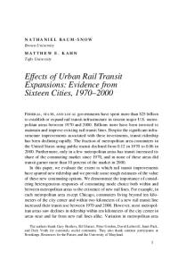
Figure 1: Crime rates across Chicago tracts. From left to right: total violent crime rates, homicide rates, assault & battery rates, and property crime rates. Green denotes low crime rates, red denotes high crime rates. day are workers, not residents (by my calculation over 300,000 people commute into this tract daily). It is reasonable to assume, then, that most people who are victims of crime in this tract—especially during the day—are not residents. The naive crime rate is misleading because it overestimates (in this case) the true probability of being the victim of a crime, which is the relevant statistic when assessing the crime risk in a given area. To calculate this “worker-adjusted” crime rate, I find the daytime population of each tract. The daytime population is simply the residential (“nighttime”) population plus the number of people working in the tract less the number of people who leave the tract when they go to work. I use commuting flows (along with an adjustment factor to compensate for the LEHD’s partial coverage) to calculate these numbers. I can then calculate the overall crime rate by averaging the daytime and nighttime crime rates, using the time stamp from the crime incident reports to determine when the crime was committed.13 Specifically, I calculate crime rate =

num. daytime crimes num. nighttime crimes + . daytime pop. nighttime pop.

(13)

Using this formula, the violent crime rate for the tract above drops from 2,700 to 1,460, which is intuitively more reasonable. (This modified measure still suffers from an upward bias as it neglects to account for tourists and other leisure visitors, of which there are many; but this is only a problem for a very small number of tracts.) Parameters

I set 1 − 𝛽 = 0.31, consistent with the empirical fact that the median expenditure

on rent in the Chicago metro area was roughly 31% in the 2015 ACS. I use the Bureau of Labor Statistics’ American Time Use Survey (averaged over the period 2011-2015) to estimate 𝛽ℓ , noting that 𝛽ℓ is the ratio of time spent in leisure activities to time spent working. I define working as 13

“Daytime” is between 6 AM and 6 PM, while “nighttime” is between 6 PM and 6 AM.

11

Violent Homicide (1st or 2nd degree) Aggravated assault or battery Firearm battery Robbery Criminal sexual assault Street violent crime Non-street violent crime Property

Total 110,321 2,124 44,170 8,477 57,844 6,093 75,941 34,290 495,151

Tract rates (per 100,000) Mean 25th 50th 75th 1043 347 659 1475 19 0 7 25 409 122 257 551 75 6 27 108 565 182 349 769 52 20 37 72 719 223 455 994 325 121 198 447 4546 2386 3579 5627

Table 1: Distribution of tract crime rates (per 100,000 population) in Chicago. Mean and quantiles are weighted by population, using simple (“naive”) crime rates. Totals are over 5-year period. all non-commuting work-related activities,14 while all remaining activities, with the exception of “personal care” (mostly sleeping and grooming) are considered leisure. This yields 𝛽ℓ = 4.96 for the average American over the period of interest. The average daily time spent on leisure, working, and commuting combined was 14.45 hours; therefore, in the expression for 𝑑𝑖𝑗 , the commuting time share is given by 𝜏𝑖𝑗𝑐 = 𝑡𝑖𝑗 × (2 × 5/7)/(14.45 × 60), where I assume that workers commute five out of seven days each week.15 I will back out the Fréchet shape parameter 𝜃 from the gravity regression in the next section. I assume, for the time being, that housing supply is fixed (𝛾 = 1). It is difficult, at this stage in the project, to estimate 𝛼𝑖 —which is driven by, among other things, zoning laws and geological constraints—for each location. Saiz (2010) does suggest a way forward in estimating the elasticity of housing supply; for now, I fix housing supply and treat my results as conservative short-run estimates.

4 Estimation results 4.1 Gravity I perform OLS regression on the linearized gravity equation (6), limiting my sample to origindestination pairs with positive commuting flows (𝑁 = 1.9 million), which yields 𝜃 = 3.54. Recall that 𝜃 controls the heterogeneity of commuter preferences: a higher 𝜃 implies lower heterogeneity; certain subpopulations will generally be less heterogeneous. We would expect, therefore, that performing the gravity regression on the subset of commuting pairs corresponding to residential and workplace locations in Chicago proper would yield a higher 𝜃; indeed, this regression gives 𝜃city = 5.52. The value of 𝜃 backed out from the full-sample regression implies that, in the case where there is no new residential construction, the population elasticity with respect to amenity, 𝜎, is 1.69; that 14 15

The ATUS does not report time spent commuting, so I rely on estimates from ACS. Strictly speaking, the round-trip commuting time is 𝑡𝑖𝑗 + 𝑡𝑗𝑖 , but I will assume symmetry in travel times.

12

log(amenity) (1) log(violent)

(2) ∗∗∗

(3)

(4) ∗∗∗

−0.250 (0.008)

(6) ∗∗∗

−0.343 (0.013)

(7)

(8) ∗∗∗

−0.110 (0.010)

−0.279∗∗∗ 0.210∗∗∗ (0.019) (0.023)

log(property)

−0.130 (0.017) −0.106∗∗∗ (0.014)

0.033 (0.022)

−0.308∗∗∗ (0.017)

log(combined) Controls Observations 𝑅2adj

(5)

Exog 781 0.673

Exog 781 0.431

Exog 781 0.705

Exog 781 0.497

−0.115∗∗∗ (0.014) All 781 0.788

All 781 0.772

All 781 0.788

All 781 0.775

Note: ∗ , ∗∗ , ∗∗∗ Significant at the 10, 5, and 1 percent levels, respectively.

Table 2: Results of (log) amenity regressions on (log) violent and property crime. is, a 1% increase in amenity leads to a 1.7% increase in population at a given location. Using data on housing prices 𝑟𝑖 , I can then back out residential amenity 𝐵𝑖 for each tract.16

4.2

Amenity regressions

I regress the log of residential amenity on several breakdowns of crime rates and controls. Table 2 shows the results of the first set of these regressions. When I include only exogenous controls (that is, control variables that are unlikely to be influenced by crime rates), the effect of violent crime is significant: a 10% increase in the violent crime rate reduces amenity by 2.5%, which would translate to a 4.2% drop in population (assuming the crime spike is localized). However, adding the remaining controls more than halves these figures to 1.1% and 1.9%, respectively. The latter can be seen as a conservative short-run estimate of the effect of violent crime, and this is the figure that I will use later in my analysis. The 𝑅2 of 0.67 in column (1) is fairly large: when compared to a regression of amenities on exogenous controls alone (𝑅2 = 0.28), we see that violent crime can explain around 39% of the variation in neighborhood amenities beyond these controls. Although the coefficient on property crime is large and significant absent other (non-control) regressors, it is clear from columns (3) and (7) that property crime actually has a negligible effect on amenity once violent crime is accounted for. Somewhat counterintuitively, the coefficient on property crime is actually large and positive in column (3) (and small and positive in column (7)); this is likely due to the fact that the property crime rate is actually capturing the existence of potential targets of these crimes (i.e., wealthier areas with more property that can be targeted) in the absence of the full panel of controls. When all controls are introduced, the measured effect of property crime remains slightly positive but is statistically insignificant. Table 3 shows the effects of violent crime broken down by type. Note that, in this log-log specification, I set crime rates of 0 to 1.17 In column (1), it appears that homicides have a large and sig16 17

Recall that 𝐵𝑖 implicitly includes residential capacity, which I will control for in the amenity regressions. 1 is sufficiently close to 0 given the magnitudes of the crime rates; see Table 1.

13

log(amenity) (1) log(homicide)

(2) ∗∗∗

−0.133 (0.005)

(3) ∗∗∗

(4)

(5) ∗∗∗

−0.040 (0.007)

−0.043 (0.006)

(6) ∗∗∗

−0.017 (0.006)

log(assault & battery)

−0.174∗∗∗ (0.016)

−0.056∗∗∗ (0.016)

log(robbery)

−0.036∗∗ (0.015)

−0.047∗∗∗ (0.013)

0.025∗∗ (0.010)

0.006 (0.009)

log(sexual assault) log(street)

−0.224∗∗∗ (0.018)

−0.098∗∗∗ (0.016)

−0.020 (0.019)

−0.014 (0.015)

log(non-street) Controls Observations 𝑅2adj

Exog 781 0.604

Exog 781 0.716

Exog 781 0.687

All 781 0.772

All 781 0.792

All 781 0.791

Note: ∗ , ∗∗ , ∗∗∗ Significant at the 10, 5, and 1 percent levels, respectively.

Table 3: Results of (log) amenity regressions on (log) violent crime, with breakdown by type. nificant effect on amenity; this, however, is belied by the results in columns (2), (4), and (5). In fact, when all types of violent crime are included with the full panel of controls, the coefficient on homicides shrinks to statistical insignificance. It turns out that assault and robbery dominate in both columns (2) and (5). This is not surprising: although homicides are especially tragic and receive the lion’s share of media coverage, they are far less common than assaults, batteries, and robberies (see Table 1); therefore, the fear of being assaulted or robbed generally figures most prominently in the minds of residents of high-crime areas. Furthermore, it appears that a large share—if not a majority—of homicides in Chicago are gang-related. Although concrete data on gang violence are largely absent (or haven’t been made public by the CPD), national media have reported on Chicago’s gang violence extensively in recent years, especially in light of Chicago’s homicide spike in 2016. University of Chicago Crime Lab (2017) reports, using data from the CPD, that 53% of homicide victims in 2015 had gang affiliations, though this is likely a lower bound on the true number, given the indirect or unofficial nature of many of these affiliations. That said, even gang violence directed at rival gangs often affects residents who are not gang members themselves, but Table 3 suggests—though by no means proves—that perhaps this effect is relatively small, once other types of crimes and determinants of amenity are accounted for. Table 4 shows the results of log-linear amenity regressions, which sheds further light on some of these questions by considering levels of crime rates. Notice that homicides dominate in column (6), which suggests that one additional homicide has a much larger effect on amenity than one additional assault or robbery. If, for instance, a neighborhood with a population of 5,000 experiences one additional homicide (while nothing else changes), amenity will decline by around 1.2%, 14

log(amenity) Thousands per 100,000 violent

(1)

(2)

(3)

∗∗∗

(5)

(6)

−1.802∗∗∗ (0.236)

−0.587∗∗ (0.275)

∗∗∗

−0.181 (0.006)

−0.079 (0.007) −5.670∗∗∗ (0.257)

homicide

(4)

−1.271∗∗∗ (0.336) −0.449∗∗∗ (0.043)

−0.140∗∗∗ (0.039)

robbery

−0.040 (0.026)

−0.057∗∗∗ (0.022)

sexual assault

0.660∗∗∗ (0.250)

0.140 (0.206)

assault & battery

Controls Observations 𝑅2adj

Exog 781 0.652

Exog 781 0.557

Exog 781 0.686

All 781 0.791

All 781 0.772

All 781 0.792

Note: ∗ , ∗∗ , ∗∗∗ Significant at the 10, 5, and 1 percent levels, respectively.

Table 4: Results of (log) amenity regressions on (linear) violent crime (in thousands per 100,000 population), with breakdown by type. compared with only 0.3% for an additional aggravated assault or battery (though note that the standard error on homicides is quite large). This is a fact that Table 3 obscures, because homicide rates tend to be much lower than rates of other types of violent crime. The positive coefficient on criminal sexual assault in columns (2) and (5) of Table 3 (and columns (3) and (6) of Table 4) may seem paradoxical, but it is more easily understood in light of the high likelihood of underreporting. It seems probable that sexual assaults are more likely to be reported in lower-crime and more prosperous neighborhoods, introducing the positive bias. Columns (3) and (6) of Table 3 also shed light on this result. Violent crime’s impact on amenity is carried entirely by street crimes; it appears that residents assign little or no weight to being victimized in their homes or other private establishments, possibly because these crimes are considered more targeted and less “random.” Sexual assault is generally a non-street crime; only 18% of sexual assaults in the sample (excluding those explicitly labeled “domestic”) are committed on the street, compared to 66% of homicides, 65% of assaults, and 77% of robberies. This goes a long way in explaining the apparent paradox.

5

Quantitative analysis

5.1 City-wide crime effects I’ve established in the previous section that a 10% localized increase in violent crime reduces the population at a given location (in the short run) by 1.9%. But crime increases (or decreases) are seldom local, especially at the tract level; furthermore, amenity changes in one location might affect 15

population and housing values at other locations. The benefit of a structural model, like the one used in this paper, is that it allows us to capture these non-local effects, in this case through the multilateral resistance Φ. What would be the effect of a 10% city-wide increase in violent crime? Naturally this depends on the geographic distribution of the increase. If the increase is concentrated in neighborhoods that already have high crime rates the total impact will be smaller than if it hits all or only lowcrime neighborhoods; this is because high-crime neighborhoods generally have lower population densities and because the proportional increase in crime would be smaller (since a priori crime is already high). Using (12) and the assumption that there is no migration into or out of the Chicago metro, it can be shown that a 10% increase in violent crime across all city tracts decreases city population by 1.22%. This is very close to the size of the effect found by Cullen and Levitt (1999). Why is this figure smaller than the 1.9% localized effect? When the crime increase is localized, it is basically costless (there are no moving costs in the model) for residents to relocate to neighboring tracts; these tracts might have slightly higher rents as new residents arrive, but commuting costs remain basically unchanged for these new arrivals. When the crime increase is city-wide (or at least impacts a large part of the city), the cost of relocation is now higher, partly because moving will make residents incur higher commuting costs and partly because city rents have declined, allowing residents who stay in the city to consume more housing; therefore fewer residents are willing to make the move. When the 10% total increase is limited to tracts with above-median crime rates, city population declines by only 0.72%; when the spike is restricted to tracts with below-median crime rates, the population drops by a much larger 2.82%. This hints that there may be an incentive for cities to concentrate their police forces in neighborhoods that already have lower crime rates, given that crime spikes in these neighborhoods could do much greater harm to the city’s coffers (and the city’s economy more generally).

5.2

West Side story

Violent crime in Chicago is generally concentrated on the West and South sides of the city (see Figure 1). What would happen to the city’s population if violent crime on the West Side were reduced to 750 per 100,000, just above the city-wide median? The structural model, along with the estimated parameters, can help us answer this question. I perform three related experiments. In all experiments, I assume housing stock is fixed (𝛾 = 1); I also assume the conservative estimate for the impact of violent crime—i.e., that a 10% crime reduction increases amenity by 1.1%. In the first experiment, I limit migration to the city of Chicago; that is, all new residents arriving on the West Side come from other parts of Chicago, so the total population of the city is unchanged. In this case, the population of the West Side grows by 55,100, or 11.4%. In the second experiment, I allow within-metro migration but prohibit migration into the metro area; now the West Side population grows by 64,300 (13.3%) and the Chicago population grows by 47,000 (1.7%). In the third experiment, I allow migration into the metro area as well; to do 16

this, I fix 𝜋̂𝑅𝑖 = 1 for tracts 𝑖 outside the West Side that have seen no changes in residential amenity (since we assume that metro outsiders will move to these areas until the population is the same as before). In this case, the West Side population grows by 68,500 (14.2%); Chicago’s population grows by the same amount since the populations of tracts outside the West Side are unchanged. If I use the high-end estimate for the crime effect (amenity elasticity of −0.25 with respect to violent crime), the West Side population would actually grow by 177,300 (36.8%). This figure should be interpreted cautiously: on the one hand it relies on amenity and infrastructure improvements not driven primarily or exclusively by decreases in violent crime, but on the other hand it also assumes fixed housing supply, which in the long run is an exceedingly conservative assumption.

6

Conclusion

Unsurprisingly, urban crime—primarily violent crime—is an important driver of residential amenity in cities, which in turn plays a major role in determining a metro area’s residential patterns. For Chicago I find that a 10% localized increase in the violent crime rate decreases amenity by 1.1% and population by 1.9%, though larger-scale changes in crime rates have more complicated effects on in- and outmigration, as I show in the previous section. My estimates suggest that the disamenity of crime is driven by violent, not property, crimes, and that, among violent crimes, aggravated assaults and batteries dominate (though individual homicides can play a large role as well). I emphasize that these estimates are likely conservative, because (i) they neglect changes in other amenities that might be driven, at least in part, by crime rates and (ii) they assume fixed housing supply. A natural extension of my analysis—and one I am currently implementing, leveraging incomedisaggregated data from the LEHD—would allow us to distinguish between low- and high-income residents, who generally have different consumption behavior (especially in housing expenditure) and likely have different responses to crime. It would also shed light on phenomena like gentrification, in which higher-income residents move into recently-improved lower-income neighborhoods and outbid many of the previous residents. A similar result could be achieved by making the residents’ utilities non-homothetic in housing, though this may compromise the tractability of the model. These extensions are discussed in more detail in the Appendix.

17

References Ahlfeldt, G. M., S. J. Redding, D. M. Sturm, and N. Wolf. “The economics of density: evidence from the Berlin Wall.” Econometrica 83.6 (2015): 2127–2189. Allen, T., C. Arkolakis, and X. Li. “Optimal city structure.” Mimeo Northwestern and Yale Universities (July 2015). Alonso, W. Location and Land Use: Toward a General Theory of Land Rent. Cambridge, Harvard University Press, 1964. Baum-Snow, N. “Did highways cause suburbanization?” The Quarterly Journal of Economics 122.2 (2007): 775–805. Chicago, City of. Data Portal, data.cityofchicago.org (2016). Cullen, J. B., and S. D. Levitt. “Crime, urban flight, and the consequences for cities.” The Review of Economics and Statistics 81.2 (1999): 159–169. Eaton, J., and S. Kortum. “Technology, geography, and trade.” Econometrica 70.5 (2002): 1741–1779. Glaeser, E. L. “Learning in cities.” Journal of Urban Economics 46.2 (1999): 254–277. ——, and J. Gyourko. “Urban decline and durable housing.” Journal of Political Economy 113.2 (2005): 345–375. ——, H. D. Kallal, J. A. Scheinkman, and A. Shleifer. “Growth in cities.” Journal of Political Economy 100.6 (1992): 1126–1152. Jacobs, J. The Death and Life of Great American Cities. New York, Random House, 1961. ——. The Economy of Cities. New York, Random House, 1969. Lucas, R. E., and E. Rossi-Hansberg. “On the internal structure of cities.” Econometrica 70.4 (2002): 1445–1476. McFadden, D. “The measurement of urban travel demand.” Journal of Public Economics 3.4 (1974): 303–328. Mills, E. S. “An aggregative model of resource allocation in a metropolitan area.” The American Economic Review 57.2 (1967), 197–210. Muth, R. F. Cities and Housing: The Spatial Pattern of Urban Residential Land Use. Chicago, University of Chicago Press, 1969. Newberry Library. “Chicago Homicide Rates per 100,000 residents, 1870–2000”. The Encyclopedia of Chicago. Chicago, University of Chicago Press, 2004. 18

Roback, J., “Wages, rents, and the quality of life.” Journal of Political Economy 90.6 (1982): 1257–1278. Saiz, A. “The geographic determinants of housing supply.” The Quarterly Journal of Economics 125.3 (2010): 1253-1296. Santos Silva, J.M.C., and S. Tenreyro. “The log of gravity.” The Review of Economics and Statistics 88.4 (2006): 641–658. Thaler, R. “A note on the value of crime control: evidence from the property market.” Journal of Urban Economics 5.1 (1978): 137–145. University of Chicago Crime Lab. Gun Violence in Chicago, 2016 (2017). U.S. Census Bureau. 2010 Census of Population and Housing, Population and Housing Unit Counts. U.S. Government Printing Office, 2012. ——. 2015 American Community Survey 5-Year Estimates, www.census.gov/programs-surveys/acs (2016). ——. Longitudinal Employer-Household Dynamics (LEHD) Origin-Destination Employment Statistics (LODES), lehd.ces.census.gov/data (2017). U.S. Department of Justice, Federal Bureau of Investigation. Crime in the United States, 2014 (2015). U.S. Department of Labor, Bureau of Labor Statistics. American Time Use Survey, 2011-2015 (2015).

19

Appendix A.1

Model extensions

In this section I outline several model extensions that guide current and future work on this project. Heterogeneous agents The baseline model outlined in the second section does not distinguish between workers on the basis of income class or skill group; the idiosyncratic preference shock 𝑧𝑖𝑗 implicitly captures these differences. One of the harsh realities of urban crime—past and present— is its disproportionate impact on poorer residents, as these residents usually have more limited mobility. Consequently, when crime is reduced in a given area, higher-income residents generally have a stronger response and lower-income residents might be priced out altogether (this is what is often called “gentrification”). To capture this income-specific effect, we can rewrite (4) as 𝑔 𝑔

𝑔 𝜋𝑖𝑗

𝑔

𝜃𝑔

⎛ 𝐵𝑖 𝐸𝑗 𝑤𝑗 ⎞ ⎟ ⎜ ∝⎜ ⎟ ⎜ 𝑔 1−𝛽𝑔 ⎟ 𝑑 𝑟 ⎠ ⎝ 𝑖𝑗 𝑖

,

(14)

where 𝑔 ∈ {𝐿, 𝐻} indexes for the income group (low or high). Notice that I allow all parameters and variables other than housing price (which is objective and location-specific) to vary across income groups. Specifically, high and low income groups might have different assessments of location desirability, certainly different wages, and likely different commuting costs (low-income groups often depend heavily on public transit). They are also likely to have different parameter values: low-income residents generally spend a larger share of their income on housing (1 − 𝛽𝐿 > 1 − 𝛽𝐻 ) and have less heterogeneous location preferences (𝜃𝐿 > 𝜃𝐻 ); they are therefore likely to have different population elasticities 𝜎, and will likely have differential responses to changes in crime rates. Non-homothetic housing preferences In lieu of (or in addition to) using different values of 𝛽 to account for differences in housing expenditure share across income groups, we can introduce a non-homotheticity into the worker’s utility function. For tractability, this approach would require me to drop the leisure term in the utility function and replace it with a general commuting cost function 𝑑𝑖𝑗 , which can be an exponential function of commuting time, as in Ahlfeldt et al. (2015). (1) then becomes 𝑢𝑖𝑗 (𝜔) =

𝐵𝑖 𝐸𝑗 𝑑𝑖𝑗

𝑞𝑖𝑗 (𝜔)𝛽 (ℎ𝑖𝑗 (𝜔) − ℎ)̄ 1−𝛽 𝑧𝑖𝑗 (𝜔),

where ℎ̄ is the minimum quantity of housing each worker must consume. This implies that workers will consume ℎ𝑖𝑗 = (1 − 𝛽)𝑤𝑗 /𝑟𝑖 + 𝛽ℎ̄ units of housing and 𝑞𝑖𝑗 = 𝛽𝑤𝑗 − 𝛽𝑟ℎ̄ units of the final good.

20

The gravity equation (4) becomes 𝜃 𝐵𝑖 𝐸𝑗 (𝑤𝑗 − 𝑟𝑖 ℎ)̄ ⎞ ⎛ ⎟ 𝜋𝑖𝑗 ∝ ⎜ ⎜ ⎟ . 1−𝛽 𝑑 𝑟 𝑖𝑗 𝑖 ⎝ ⎠

Notice that 𝜋𝑖𝑗 now scales with the difference between the wage at 𝑗 and the minimum housing expenditure required to live at 𝑖. Low-income workers may not be able to afford the minimum quantity of housing ℎ̄ in neighborhoods with high 𝑟𝑖 , helping us match the observation that poorer residents are typically concentrated in neighborhoods with lower housing prices (and lower-quality amenities). Agglomeration effects

Much of the recent literature in urban economics, notably Ahlfeldt et al.

(2015) and Allen et al. (2015), has emphasized the importance of agglomeration effects in models of urban geography. In the context of residential decisions, agglomeration effects can increase amenity by, for instance, stimulating social and productivity-improving interactions with neighbors. The agglomeration coefficient at 𝑖 can be written as 𝜓𝑖 = ∑ 𝑒−𝜌𝑡𝑖𝑟 𝜋𝑅𝑟 , 𝑟

where 𝜌 > 0 captures the rate at which these effects decay with distance. While it is straightforward, in principle, to estimate the impact of agglomeration effects (once 𝜌 is known), it complicates the comparative statics analysis, since the general equilibrium must be solved from scratch whenever amenities change. Qualitatively, agglomeration effects can compound the magnitude of crime reduction effects, as population increases themselves make a location more desirable in something of a virtuous cycle. Crime increases, in contrast, can initiate a vicious cycle in this model, matching what we often see in practice as well.

21