IEEE TRANSACTIONS ON MULTIMEDIA, VOL. 15, NO. 3, APRIL 2013

633

Video-to-Shot Tag Propagation by Graph Sparse Group Lasso Xiaofeng Zhu, Zi Huang, Jiangtao Cui, and Heng Tao Shen

Abstract—Traditional approaches to video tagging are designed to propagate tags at the same level, such as assigning the tags of training videos (or shots) to the test videos (or shots), such as generating tags for the test video when the training videos are associated with the tags at the video-level or assigning tags to the test shot when given a collection of annotated shots. This paper focuses on automatical shot tagging given a collection of videos with the tags at the video-level. In other words, we aim to assign specific tags from the training videos to the test shot. The paper solves the V2S issue by assigning the test shot with the tags deriving from parts of the tags in a part of training videos. To achieve the goal, the paper first proposes a novel Graph Sparse Group Lasso (shorted for GSGL) model to linearly reconstruct the visual feature of the test shot with the visual features of the training videos, i.e., finding the correlation between the test shot and the training videos. The paper then proposes a new tagging propagation rule to assign the video-level tags to the test shot by the learnt correlations. Moreover, to effectively build the reconstruction model, the proposed GSGL simultaneously takes several constraints into account, such as the inter-group sparsity, the intra-group sparsity, the temporal-spatial prior knowledge in the training videos and the local structure of the test shot. Extensive experiments on public video datasets are conducted, which clearly demonstrate the effectiveness of the proposed method for dealing with the video-to-shot tag propagation. Index Terms—Manifold learning, sparse coding, sparse group lasso, structure sparsity, video annotation, video tagging.

I. INTRODUCTION

T

HE issue of video tagging (a.k.a. “high-level feature extraction” or “concept detection” [1]–[4]) is well known as to automatically annotate video data with textual description of semantic concepts, such as objects, locations or activities. However, most of the existing methods on video tagging are only focused on propagating the tags or the concepts at the same level, such as the literatures in [5], [6], while a more fine-grained tagging at the shot level via learning from video-level tags is also important in many real applications.

Manuscript received February 01, 2012; revised June 04, 2012 and August 05, 2012; accepted August 07, 2012. Date of publication December 12, 2012; date of current version March 13, 2013. This work was supported in part by Australia Research Council DP1094678 and in part by the National Natural Science Foundation of China Under Grant No. 61173089. The associate editor coordinating the review of this manuscript and approving it for publication was Dr. Chong-Wah Ngo. X. Zhu, Z. Huang, and H. T. Shen are with School of Information Technology and Electrical Engineering, The University of Queensland, Brisbane, Australia (e-mail: [email protected]; [email protected]; [email protected]). J. Cui is with the School of Computer Science, Xidian University, Xian, China. Color versions of one or more of the figures in this paper are available online at http://ieeexplore.ieee.org. Digital Object Identifier 10.1109/TMM.2012.2233723

Fig. 1 shows an example video clip of Queensland flood consisting of three shots. The provided video-level tags are “Queensland flood”, “clean-up”, “urban”, “river side”, and “car”. By performing video-to-shot tag propagation, the tag “clean-up” is assigned to the last shot, which will be directly retrieved while searching for the event of “clean-up”. By assigning tags to shots, the content of interest can be retrieved efficiently without the scan against entire videos. In this paper we aim to address the problem of propagating the known video-level tags to specific shots, and call such an interesting topic the V2S issue. We also define the process of tag propagation as the one assigning the shots with tags based on the video-level tags. Moreover, the process does not care whether the test videos containing the test shots have tags. Due to the expensive labor cost, it is not practical to implement tag propagation manually. Thus efficient and accurate tagging methods are in high demand. Unfortunately, most existing methods of video tagging (e.g., [7], [8]) focus on propagating tags at the same level. For example, given a collection of training videos with tags at the video level, the test video can only be annotated at the video level while the tags of its individual shots cannot be specified. While treating a video as a bag (i.e., a bag of frames), multiple instance and multi-label (MIML) learning [9], [10] could be applied. However, video data is a complex data type containing visual and temporal information, which cannot be handled by the simple MIML models. Hence, to solve the V2S issue is practical as well as challenging. In this paper, we format the V2S issue as a reconstruction model by which we find the correlations of visual features between the test shot and the training videos. The derived correlations are used to propagate the tags of the training videos to the test shot. More specifically, the paper first proposes a novel graph sparse group lasso (GSGL) method to perform shot reconstruction1 for a given test shot, by regarding the shots in the video corpus as the bases and each video as a group of shots. During the reconstruction process, we reasonably assume that the videos selected for the reconstruction process shall preserve both the intra-group sparsity (i.e., the sparsity within the group) and the inter-group sparsity (i.e., the group-wise sparsity). Moreover, the GSGL involves certain prior knowledge within the video corpus (such as spatial-temporal information of videos) and the local structure (i.e., the local structure of manifold in the domain of manifold learning) between the test shot and the video corpus, into the process of shot reconstruction. 1We define shot reconstruction as the process which linearly reconstructs the visual features of a given shot by the visual features of the known videos in this paper. Moreover, we alternately use the two concepts, i.e., test shot and query shot in this paper. So do the concepts between the training videos and the video corpus.

1520-9210/$31.00 © 2012 IEEE

634

IEEE TRANSACTIONS ON MULTIMEDIA, VOL. 15, NO. 3, APRIL 2013

Fig. 1. A video clip of Queensland flood consisting of three shots.

After the reconstruction process, we obtain the reconstruction correlation of visual features between the test shot and the video corpus, in which the visual feature of the test shot is linearly reconstructed by parts of the shots in some of training videos. We further propose a statistical model to assign the video-level tags to the test shot with the corresponding probability. Moreover, in this paper we apply the proposed solution on the V2S issue into two scenarios. More specifically, given a set of annotated videos, on the one hand, given an video with video-level tags, we aim to localize these tags to each individual shot. On the other hand, simply given a test shot, we assign it with semantic tags automatically. The contributions of the proposed solution for solving the V2S issue are presented as follows: • The paper proposes an efficient solution to the V2S issue, by extending the previous work [11]. The proposed solution casts the V2S issue as a reconstruction process in which the test shot is represented by parts of shot in some of the training videos. • The proposed GSGL method simultaneously considers the intra-group sparsity and prior knowledge in one video, the inter-group sparsity across the videos, and the local structure of the test shot. Its objective is to enforce the information for the reconstruction process. Although some lasso-style methods (such as, lasso [12]–[14], group lasso [15] and sparse group lasso [16], [17]) can be developed to reconstruct the test shot by the training videos, to the best of our knowledge, the GSGL is the first work that simultaneously considers these four constraints within one single reconstruction model. Moreover, the GSGL is the first model considering the local structure of the video corpus into the framework of the sparse group lasso. • Extensive experiments are conducted on real data sets to illustrate the effectiveness of our proposal. The results show that the proposed method outperforms the state-of-the-art and baseline algorithms for dealing with the V2S issue in terms of average precision and Hamming loss on the tagging assignments. In the rest parts of the paper, we briefly review the related literatures on video tagging in Section II. The following sections are the notations, the preliminary and the details of the proposed method for solving the V2S issue respectively. The experimental results are shown in Section VI followed by the conclusion in Section VII. II. RELATED WORK Many learning models and systems have been proposed to automatically assign keywords or concepts onto videos, such as

the literatures [18], [19]. In this section, we give a brief review of existing methods on this topic. Video tagging (or annotation) can usually be formulated as multiple instance and multi-label (MIML) learning over individual videos or shots, via employing different kinds of learning models, such as multi-label learning [7], [20], active learning [21], [22], online learning [2], [23], and so on. Traditional methods on video tagging can be categorized into the methods over individual shots and the methods over sequential shots [8]. The existing work on the methods over individual shots detect concepts within individual shots independently to exploit all kinds of correlations of concepts within individual shots via different methods, such as a random walk in [24] and multi-label classifiers in [7]. Recently some learning models (such as multiple concept detectors [25] and multi-label classifiers [7]) are used to learn the relationship among tags at the shot level, by treating video shots as independent instances. To further improve the performance of video tagging, a lot of research has been done to exploit the spatial correlations among tags within each shot via machine learning methods, such as Bayesian network [26], conditional random fields (CRF) [27], among others [28]. Actually, the study on the video tagging over individual shots are only the extension of image annotation methods to video domain [8] because they treated tags (or concepts) within individual shots independently, while the temporal information embedded in the videos is ignored. In real applications, the video is usually temporally informative, thus researchers attempt to utilize temporal information to enhance video tagging. By regarding the temporal information in the videos into the process of video annotation, Lie et al., [8] categorized the existing methods working on the sequential shots into three categories, including the only-temporal methods, the temporal-after-annotation methods and the spatial-temporal methods. The only-temporal methods (e.g., [7], [29], [30]) were designed to only model the temporal information into the learning process via machine learning methods. For example, Xie and Chang [29] modeled the temporal dynamics of low-level features (e.g., color and motion) for specific video event detections via hidden Markov models (HMM); Yi et al. [30] regarded the sequence of shots in videos as a chain structure via the conditional random field method; Qi et al. [7] modeled the similarity between sequences of low-level features as a temporal kernel. Gargi and Yagnik [31] used a wavelet decomposition of frame-level feature time-series to simultaneously learn discriminative features and their temporal support while remaining independent of position within the videos. The temporal-after-annotation methods (e.g., [32], [33]) were designed to refine the temporal consistency after annotating the individual shots. For example, Liu et al. [32] incorporated temporal consistency into active learning to detect multiple video concepts; Wang et al. [33] achieved the similar objective for refining the tags (or the concepts) via random walk. The spatial-temporal methods were designed to simultaneously model the spatial and temporal information. For example, Ebadollahi et al. [34] simultaneously used the spatial and temporal contexts of higher-level concepts to assist event/action

ZHU et al.: VIDEO-TO-SHOT TAG PROPAGATION BY GRAPH SPARSE GROUP LASSO

detection; Naphade et al. [26] took the spatial co-occurrence and the temporal dependency of tags into account for modeling the pair-wise relationships of tags via a probabilistic Bayesian network; Weng et al. [35] proposed several fusion methods to model spatial correlations and temporal consistencies of concepts; Li et al. [8] proposed a unified learning framework to capture both spatial and temporal correlations of semantic concepts by formulating video annotation as a sort of sequence multi-labeling issue. Unsupervised learning is also widely used in video tagging. For example, Siersdorfer et al. [5] first detected the duplication and overlap between two videos, and then designed two automatic tagging rules for propagating the video-level tags to a new coming video; Following the former work, Zhao et al. [6] focused on efficiently searching for similar videos by local features such that the tags from similar videos can be effectively recycled for tagging. However, both of them are focused on propagating video tags at the same level. III. NOTATIONS A. Notations and Video Representations In this paper, the vector norm (i.e., ) of the vector is defined as , where the of the vector is defined as . The matrix norm (i.e., ) of a matrix is defined as

.

B. Video Representation Given the video corpus containing training videos , we extract the visual feature of each video with shots2 , , , where is the dimensionality of the feature space representing shots. Thus, , where means the total number of the shots in . To consider all shots as a whole, we can also represent the video corpus as , where , represents a shot. Different visual features can be used for shot representation according to the different applications. In this paper, we describe shots by 256-dimension (256-D) Local Binary Pattern (LBP) features. To further capture the characteristics of videos, we also keep the duration of every shots and denote this temporal vector as . A binary matrix is designed to store the tags of each video, where is the total number of unique tags in the training videos. when the -th tag in the vocabulary appears in the -th video. Otherwise, . IV. PRELIMINARY In this section, we analyze the advantages and disadvantages of existing lasso-style methods (such as the lasso, the group 2Each

shot is represented by its key-frame.

635

lasso and the sparse group lasso) to show the motivation of the proposed method in this paper.

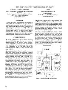
A. Lasso The reconstruction estimation for the given data can be obtained by minimizing a loss function under penalized constraints (or regularization terms). The reconstruction estimation of lasso (i.e., Least Absolute Shrinkage and Selection Operator, in [12]–[14]) is defined as follows: (1) where represents the test shot, represents the bases (in this paper, the bases are the training videos), and is the sparse codes of the (a.k.a., the weight of bases, or the coordinates of the test shot in the training videos). is a trade-off parameter. Usually, the larger value of shrinks its corresponding sparse codes to zero. Ideally, the “pseudo norm” (i.e., , a.k.a., ) means to count the total number of nonzero elements in a vector. The is a perfect sparsity but its solution is NP-hard [13]. Usually, the is employed to approximate the in real applications since it can also generate many zero elements as well as is with obviously computational benefits. Moreover, it is convex and has been shown that its results are identical or approximately identical to the corresponding results under practical conditions [13], [16]. The reconstruction estimation in (1) with the penalty is also called as basis pursuit [14]. While applying to the V2S issue, the lasso needs to be further improved. First, the lasso tends to make the selection based on the strength of individual variables (i.e., shots of the training videos) rather than the others strength, such as the groups of input variables (i.e., videos). This often results in selecting more variables (shots) to represent the test shot than necessary. Second, the lasso with regularizer generates the element-sparsity (such as Fig. 2(a)) thus the test shot is represented by the shots rather than videos. In this case, although the lasso can sparsely represent the test shot, it selects more videos, e.g., selecting totally three shots from both two training videos in Fig. 2(a). That will result in more computational cost and introduce more noise. Moreover, such a representation ignores the group effect inherent in the video. That is, the video consisting of several shots should be regarded as one group. Or the test shot should be represented by the video rather than the shots since we only have the tags of the video-level. Third, the solution of the lasso depends on how the factors are orthonormalized [15]. If any factor is reparameterized through a different set of orthonormal contrasts, the lasso may obtain a different set of factors in the solutions. So the orthonormal constraint in the lasso is not practical in real applications. Due to the limitations of the lasso aforementioned, our first motivation is to generate the video-level sparsity, i.e., the intergroup sparsity. Existing group lasso helps us to achieve it.

636

IEEE TRANSACTIONS ON MULTIMEDIA, VOL. 15, NO. 3, APRIL 2013

Fig. 2. An illustrative on three sparse learning models for comparing their sparsity. In this example, the video corpus contains two training videos consisting of three shots and two shots respectively. The test shot is supposed to be reconstructed by the these two videos. (a) The lasso generates the element-sparsity (i.e., zero element) through the whole column. (b) The group lasso generates the inter-group sparsity (i.e., the sparsity through the group), such as the sparsity in the second video but not in the first video. (c) The sparse group lasso (including the proposed graph sparse group lasso) generates the inter-group sparsity as well as the intra-group sparsity, i.e., the sparse group lasso first selects the inter-group sparsity (i.e., the second group), then generates the element-sparsity in the non-zero group (i.e., the first element in the first group).

B. Group Lasso According to the literature [15], with a vector a symmetrically positive definite matrix define:

and , we can

(2) Given the bases, trices

, and positive definite ma, the group lasso is defined as: (3)

where . The regularizer (we call it “ norm” in this paper) penalizes all regression coefficients in one group as a single feature. Thus it leads to the inter-group sparsity, i.e., the sparsity through the whole group while its corresponding is large enough. The first interesting characteristic on the in the group lasso is that we have many reasonable choices for the kernel matrices . For example, while setting (where is a constant and is an identity matrix), the reguis the , i.e., larization . Such a derived regularizer ensures to generate the inter-group sparsity. The second interesting characteristic is that we can include different kinds of useful prior knowledge into the objective function. For example, we can include prior knowledge into and we will address the details in Section V-B. Considering all the elements in one video as a whole group makes the group lasso lead to the scenario in which all the sparse codes in one video are zeros. This assures that the test shot is represented by the training videos rather than their shots, such as Fig. 2(b) where the text shot is represented by the second video only. We call such a sparsity as the inter-group sparsity (or the group-wise sparsity) in this paper. However, the group lasso does not yield the sparsity within a group. That is, if the coefficient vector for the video

(e.g., the first video in Fig. 2(b)), the value in the vector tend to be nonzero. In this way, the group lasso tends to automatically include all the shots in the video (i.e., all the shots in the second video in Fig. 2(b)) to represent the test shot once the video is selected. So the redundant noise (or the irrelevant shots to the test shot) maybe be included into the process of the shot reconstruction. In real applications, the tags of a video are usually compressed, so the test shot should be represented by parts of shots in the videos [37]. We call such a sparsity as the sparsity within the group or the intra-group sparsity. Besides without inducing the intra-group sparsity, the group lasso also does not relax the constraint of orthonormalized factors as appearing in the model of the lasso [17]. C. Sparse Group Lasso To overcome the above two drawbacks found in the group lasso, the sparse group lasso (e.g., [16], [17]) was designed by adding an norm regularizer into the original group lasso for achieving both the inter-group sparsity and the intra-group sparsity, as well as relaxing the constraint of orthonormalized factors. The sparse group lasso is defined as:

(4) where , the first regularizer penalizes the whole reconstruction error of all encoding shots, i.e., to control the overall sparsity of the reconstruction model (or the intragroup sparsity), and the second regularization term achieves the inter-group sparsity. The sparse group lasso includes both the lasso (i.e., ) and the group lasso (i.e., ). It combines regularizer and regularizer together to select only part of shots from a small number of training videos whose shots are mostly highly correlated to the test shot. The sparse group lasso is more suitable for the V2S issue than either the lasso or the group lasso. With the sparse group lasso, a training video will not be selected to represent the test shot if the corresponding is shrunken to 0. Take Fig. 2(c) as an example, only the first video is selected to represent the test video. In the meanwhile, only part of shots are used for shot reconstruction. In summary, the sparse group lasso just selects a small number of videos whose shots mostly have strong correlations with the test shot for the shot reconstruction. The unrelated shots from the selected videos are also ignored. However, further improvement on the sparse group lasso is desired. First, the sparse group lasso penalizes each factor with same weight as the lasso and the group lasso. That is, same weight for each component on (or ) is used to assess their relative importance. In real applications, this will also produce bias towards the large coefficients. Second, we expect to take advantages of prior knowledge (i.e., the spatial-temporal information in the training videos, the local structure of the test shot) to strengthen the performance of the shot reconstruction. V. APPROACH This section first describe the framework presented in Fig. 3 of the proposed method for handling the V2S issue. Then we

ZHU et al.: VIDEO-TO-SHOT TAG PROPAGATION BY GRAPH SPARSE GROUP LASSO

637

Fig. 3. The framework of the proposed approach for handling the V2S issue. The first step includes the process of shot extraction, the process of the visual information extraction of the shots, the process of tag parse, and the process of the temporal information extraction. The following steps are shot reconstruction and tag propagation respectively.

focus on the details of the second step including the details on the proposed method and its implementation. Finally, we talk about the proposed tag propagation rule. A. Framework As shown in Fig. 3, the proposed framework includes three steps, video preprocessing (i.e., tag extraction and shot extraction), shot reconstruction and tag propagation. In more detail, we first extract the tags and detect the shots of the training videos. As introduced in the previous section, the LBP feature is used to represent videos, denoted as . The tag matrix of the video corpus is denoted as . The vector records the temporal information of each video. In the second step, we perform the shot reconstruction by proposing a novel graph sparse group lasso model (GSGL), which is the key step for solving the V2S issue in this paper. Given a column vector (i.e., the visual feature vector) of the test shot, we consider the visual features of the video corpus as the bases where there are bases (i.e., totally shots in the video corpus). Moreover, each video is regarded as one group. That is, there are groups (i.e., videos) consisting of variables. The objective of the proposed GSGL is to approximately represent the visual feature of the given shot by the visual features of part of videos in the video corpus. To effectively solve the V2S issue, we expect to take advantage of the inherent prior knowledge of the data for finding correlated videos to the test shot. The inherent prior knowledge usually obtained without any cost includes the inherent structures of the data (e.g., a video as a group), the spatial-temporal information in the training videos, the local structure of the test shot, and so on. Therefore, the proposed GSGL takes into account two important constraints, such as inter-group sparsity and intra-group sparsity, and prior knowledge among the training videos. These constraints strengthen the extracted relationship between the training videos and the query shot. For example, the sparsity constraint makes the proposed solution use a part of shots (induced by the ) in a part of training videos (induced by the ) to represent the test shot. This can decrease the complexity of the algorithm and the adverse impact of the

noise. The local structure makes the shot reconstruction represent the test shot with the videos as similar as possible to it. The constraints (e.g., the group sparsity and the temporal-spatial information of the video) preserve the inherent characteristics of the video. For example, one video consisting of several shots should be regarded as a whole group, which is ensured by the group sparsity, i.e., decided by the . After the shot reconstruction, the GSGL outputs the sparse codes of the test shot , which is actually the correlation between the test shot and the video corpus. In the step of tag propagation, the tags of the test shot are obtained by combining its sparse codes and the temporal information of the training videos. Note that the derived relationship is only the one between the test shot and part of the shots in the parts of the video corpus due to the introduction of the inter-group sparsity and the intra-group sparsity. Therefore, the tags of the test shot can be efficiently propagated from the tags of part of the shots in a small number of the training videos. B. Graph Sparse Group Lasso (GSGL) To consider the temporal-spatial information into the solution to the V2S issue, we assign a temporal weight on each shot for alleviating the bias issue and a spatial weight for penalizing non-dense videos. Both the information within individual shots (i.e., the temporal weight) and the relationship among the shots within each video (i.e., the spatial weight) are utilized for achieving an effective solution for solving the V2S problem. Such a revised sparse group lasso model was called as the weighted sparse group lasso (WSGL) [11]. Besides the temporal-spatial information carried by training videos, neighborhood information of the test shot is also considered in our model. We aim to preserve the local structure of the test shot in the original feature space after performing the GSGL. In other words, the similar training videos to the test shot in the original feature space will be also close it when representing them in sparse codes by applying GSGL. It ensures that the tags of the test shots can be propagated from its similar videos as much as possible. To achieve that, we first build the similarity vector between the test shot and the video corpus,

638

IEEE TRANSACTIONS ON MULTIMEDIA, VOL. 15, NO. 3, APRIL 2013

then combine the similarity vector into the objective function of the WSGL. The objective function of the graph sparse group lasso (GSGL) is defined as:

(i.e., variable) while the existing methods consider variables equally. The temporal weight of the -th shot in the -th video is de, while the weight vector fined as . over the the -th video is denoted as D. Spatial Weighting

(5) where and are the temporal weight and the spatial weight respectively, which will be further discussed in Section V-C and Section V-D, is the weight between the test shot and the training data and will be further discussed in Section V-E. , and is the codes of -th shot of the video corpus. The value of can be obtained via Theorem 1 defined in Section V-E. More specifically, to generate the codes (i.e., new representations) for each training shot , we regard as in (8) and denote as the matrix without the training shot . Therefore, in (8), matrix does not contain the vector , i.e., while optimizing . The length of vector is because it does not contain , i.e., . Finally, we obtain via Theorem 1. Note that the process for calculating the values of is off-line. In shot reconstruction, the GSGL regards the entire video corpus as the basis space, where each video is naturally a group consisting a set of variables, i.e., shots. Given a test shot , the GSGL aims to reconstruct by the shots from via taking into account the predefined weights on each shot. The weighting issue is the key point to distinguish our GSGL method from the conventional sparse group lasso method. Moreover, the proposed method includes prior knowledge within the base space. Such a flexibility in turn can produce different amounts of shrinkage for different factors. The local structure of the test shot is the key point to distinguish the proposed GSGL from our previous WSGL. The GSGL adds one more constraint (that is, the first regularization term in (5)) for achieving a better reconstruction performance. In the next subsections, we first explain the details on temporal weight and spatial weight , and then embed the local structure of the test shot into the derived objective function. C. Temporal Weighting It is natural that long shots within a video should make much contribution to the process of video tagging than short shots. In other words, given a video with a set of tags, generally, most of the tags could be used for describing the content of the long shots. Thus, in the process of shot reconstruction, long shots with stronger association with the video-level tags, are preferred to provide a better performance on shot tagging. By taking into account this issue, we define the temporal weight for each shot

Besides the temporal information extracted from individual shots, we also consider the spatial information within each video. Spatial Standard Deviation (SSD) is applied to reveal the intrinsic relationships among the shots in a video. For the -th video consisting of shots, its SSD is formally defined as , where is the -th key frame and is the mean frame feature vector of the -th video, and the superscript stands for the -th dimension of the corresponding vectors. According to the mathematical meaning of the standard deviation, the smaller the is, the closer the shots in the -th video are. The video with a small SSD is called dense video (or dense group). We assume that dense videos should be selected with higher priority resulting in a higher group sparsity in shot reconstruction. Less the videos being selected can reduce the noise introduced to the reconstruction model to some extend. Thus, the SSD can be used as a penalty to the non-dense videos in the GSGL model. In this paper, such an SSD is formally called spatial weight, which is denoted as . That is, is a normalized vector of . E. Local Structure Video corpus are used as the bases for reconstructing the test shot, so the basis space is the space spanned by the videos. According to the theory on manifold learning [38], [39], it is important to preserve the original local structure of the test shot in the basis space. In other words, preserving the local structure makes the test shot could be represented by its similar shots or videos. More specifically, in the training process of the V2S issue, we map training data into the basis space to obtain their new representations , while assuring that the local structure of is preserved in the basis space, according to the principle of manifold learning. In the test process, following by existing literatures, such as [39], [40], we also expect to make the local structure of the test shot be preserved in the basis space, for obtaining better performance. For achieving these objectives, following Gao et al., [40], we employ graph to characterize the local structure of data and add the constrain of Laplacian graph (i.e., the second term in (5)) to achieve the local structure preservation. Note that Gao et al., [40] added Laplacian graph constraint in the objective function of lasso while ours is designed for space group lasso. To generate a -nearest-neighbor graph for the video corpus, ( we use a heat kernel is a tuning parameter, we set in this paper) to build a weight matrix . The value of is used to measure the closeness of the visual features of two shots and , and we set to avoid the problem of scale in this paper. Given a weight matrix , we use the Euclidean distance to measure the smoothness between and , where (or )

ZHU et al.: VIDEO-TO-SHOT TAG PROPAGATION BY GRAPH SPARSE GROUP LASSO

is the projection of the -th shot (or -th shot) in the new space spanned by the video corpus, that is,

639

Note that since is a positive-definite matrix, we can solve by the Cholesky decomposition method presented in [41]. After the transformation via Theorem 1, we set , , the objective function in (5) is converted into

(6) We denote as a diagonal matrix. The entries of are the column (or row, since is symmetric) sums of , i.e., . Thus is a Laplacian matrix. Usually, such a form defined in (6) is called Laplacian prior of the video corpus. Given a test shot, we first calculate its nearest neighbors in the video corpus and generate its similarity vector , to preserve the similarity between the test shot and each shot in the video corpus. Here we follow the idea from the literature [40]. That is, we suppose that the test shot does not affect the graph used in the video corpus, and the sparse codes for the video corpus are fixed. Hence, to build nearest neighbors of the test shot, rather than optimizing the (6), we just change it to optimize:

(7) where , is the projections of -th shot in the space spanning by the video corpus. F. Final Objective Function In this section, we first integrate the first two terms in (5), and then convert the derived results into the standard form of the sparse group lasso. This can be obtained by the following Theorem 1. Theorem 1: The optimization issue on , i.e., the first two terms in (5), is equivalent to: (8) where

, .

Proof: Denote have:

, according to (7), we

(9)

(10) where . In the GSGL, each weight coefficient implies the contribution of the corresponding component to the reconstruction model. First, the weighted -norm is used to penalize each shot such that the coefficients of irrelevant shots (i.e., with higher weight) are shrunken to zero. At the same time, the weighted -norm reduces the shrinkage bias towards the larger coefficients of significant variable. Second, the weighted -norm penalizes the coefficients of significant videos such that the dense videos are firstly selected. Moreover, the local structure makes the shot reconstruction to select the similar shots and videos of the test shot to represent the test shot. G. Implementation Since we convert our original objective function in (5) into the standard form of the sparse group lasso (i.e., (10)), we can solve it following the work [17], [42] and summarize our solution in Algorithm 1. More generally, after generating the form in (10), we part the general optimization procedure on the sparse group Lasso into two sequential steps, i.e., inter-group sparsity selection followed by intra-group sparsity section. In the step of inter-group sparsity selection, we check which group is not used to reconstruct the test shot , i.e., the corresponding coefficient vector is equal to zero. Otherwise, while is nonzero, it will be implemented in the step of intra-group sparsity selection. Actually, the intergroup sparsity is decided by the -norm. The step of intra-group sparsity selection first focuses on deciding whether in is equal to zero or nonzero. In this step, we will leave the group with alone, and focus on the groups with nonzero coefficient vector. More concretely, in the group with nonzero coefficient vector , we first distinguish which element is zero or not. If is zero, we will leave it alone. Then we optimize the objective function over nonzero coefficient with all other coefficients fixed to obtain the value of . The process can be achieved by employing the one-dimensional optimization method. Actually, the intra-group sparsity in the selected group (i.e., its coefficient is nonzero) is decided by the -norm. The optimization procedure continues to perform these two steps until a convergence condition is met. We give the more details on the process of the inter-group sparsity and the intragroup sparsity as follows.

640

IEEE TRANSACTIONS ON MULTIMEDIA, VOL. 15, NO. 3, APRIL 2013

“ ” if and only if “ in (11), denote we set

Algorithm 1: Sparse Group Lasso Algorithm

and

”. To do that, , then we can obtain:

Input: (12)

Out // Learn local structures offline;

Due to

, we also obtain:

according to (7);

1: Obtain

// Obtain the spatial-temporal information; 2: Calculate

and

otherwise

;

is equal to zero, we Hence, for checking whether the vector first compute the values of according to (13), then plug into (12) to obtain the value of . Furthermore, we will set if . Otherwise, we will implement the step of intra-group sparsity selection listed in the next subsection to decide which element (in nonzero vector ) would be zero or nonzero. 2) Intra-Group Sparsity Selection: Again, we need to know which element in the nonzero vector is equal to zero or nonzero. If , according to (11), we can obtain:

// Convert (5) into (10); 3: Obtain the result of (9); // Optimizing (10); 4: for // inter-group sparsity; 5:

if

6: 7:

(13)

else // intra-group sparsity;

8:

if

9:

(14) According to the definition of the subgradient equations, it needs to satisfy the condition . Hence, we first check whether the is satisfied. If so, we set . Otherwise, we optimize the objective function to obtain , i.e.,

;

10:

else

11: ; 12: 13:

(15)

end end

14: end 15: return ; 1) Inter-Group Sparsity Selection: First, for the -th video (i.e., , we denote its corresponding coand the residual efficient , we obtain the subgradient equations of the objective function with respect to the j-shot of the th video, and set the result to zero:

(11)

where

if , otherwise . , otherwise the vector , where , . Then we check whether the vector is equal to zero. According to the above subgradient equations, we know that: if

Obviously, the optimization in (15) is the sum of a convex differentiable function (i.e., first term and third term) and a separable penalty (i.e., second term). That belongs to the one-dimensional optimization problem with respect to , and the solution can be obtained by employing the existing optimization algorithms, such as, all kinds of gradients descent algorithm. In this paper, we use the fast iterative shrinkage-thresholding algorithm (FISTA), which has been proven to converge in function values as [43], [44], where is the iteration counter.3 H. Tag Propagation By solving the objective function (10), we obtain an optimal , which represents the correlation between the test shot and the corpus videos. The importance of the -th video in the shot reconstruction is measured by , which is an integration of the importance of each shot (i.e., ) within the video. The length of 3Actually, both the training process and the test process need to build nn graph (or vector) and perform sparse group lasso. In general, the complexity (where is the training size). In our of building nn graph is about experiments, to reconstruct one test shot should take time about 0.15s, 0.6s, and 42s for dataset Kodal-s, Kodal-L and TV07 respectively in a modern PC.

ZHU et al.: VIDEO-TO-SHOT TAG PROPAGATION BY GRAPH SPARSE GROUP LASSO

each shot is also taken into account. The higher the score is, the more important the -th video is to reconstruct the test shot. As each video in the corpus is associated with a set of tags, the possibility of the -th tag in the vocabulary assigned to the test shot is calculated by , where when the -th tag belongs to the -th video while , otherwise. After ranking the probability of each tag in descending order, the tags at the top ( , 5, 10 and 15 respectively in our experiments) are allocated to the test shot as the most possible tags. VI. EXPERIMENTAL ANALYSIS In this section, we evaluate the performance of the proposed GSGL with the state-of-the-art algorithms on solving the V2S issue by testing average precision (AP) and Hamming loss (HL) on two real video datasets, i.e., Kodak’s Consumer Video Benchmark dataset [45] (shorted for Kodak) and a dataset from TREC Video Retrieval Evaluation 2007 (shorted for Trecvid07). Moreover, we apply both the proposed method and the comparison methods into two scenarios. That is we perform the task of tagging the test shot extracted from the training videos as well as tagging the test shot not included in the training videos. A. Experiments Setup 1) Datasets: The Kodak dataset has 25 concepts over 1358 videos consisting of 5166 shots. The number of keyframes of Kodak varies from 5 to 40. In our experiments, the entire videos (i.e., 1358 videos consisting of 5166 shots) are considered as the first video corpus named Kodak-l, while a number of 293 videos containing no less than five shots in each video are selected as the second video corpus named Kodak-s, in which there are total 2588 shots. We select 285 shots whose number of tags is larger than two as the test dataset.4 The number of test tags varies from 2 to 5, and the average number of test tags is about 2.98. Moreover, in our experiments the test dataset is included in the dataset Kodak-l but it is not included in the dataset Kodak-s. The Trecvid07 dataset has 36 concepts over 110 videos consisting of 21532 shots. The number of keyframes of Trecvid07 varies from 5 to 881. The distribution of the concepts over 110 videos in Trecvid07 is very imbalance. For example, all 110 videos have the tags “face” and “person”. In our experiments, we delete these two tags such that there are 34 concepts in our Trecvid07 dataset. Moreover, we select all 110 videos as the video corpus and 551 shots whose number of tags is no less than seven as the test data. Finally, the number of test tags varies from 7 to 11, and the average number of test tags is about 7.5. Moreover, the test shots come from the training datasets. Kodak dataset have parts of video-level data, the left part of Kodak dataset and the Trecvid07 dataset have shot-level tags. We combine the shot-level tags of the shots in one video to form the video-level tags of this video in our experiments. Both dataset Kodak and dataset Trecvid07 provide the shots extracted and the temporal information. Therefore, in our experiments we characterize the visual content of each key frame by extracting their Local Binary Patterns (LBP) [46]. The LBP 4The

test dataset has no overlapping with the dataset Kodak-s.

641

is a type of feature used in computer vision, and is a powerful feature for texture classification. The LBP operator is defined as a gray-scale invariant texture measure, derived from a general definition of texture in a local neighborhood. In our implementation, LBP assigns a value to each pixel by comparing its 8 neighbor pixels with the center pixel value, and then transforms the result to a binary value. Furthermore, the histogram of the values is accumulated as a local descriptor. In this way, we obtain 256-dimension LBP visual features. 2) Comparison Algorithms: The proposed GSGL method simultaneously takes the factors into account, such as the intergroup sparsity, the intra-group sparsity, the temporal-spatial information and the local structure of the test shot. In the experiments, five baseline methods including NN, group lasso (GLasso) [47], Bi-layer sparse coding (LRA) [48], sparse group lasso (SGL) [17] and WSGL [11], are compared with the proposed method GSGL. • NN: NN method is a popular method on multiple instance and multi-label (MIML) learning [10]. We used it as the baseline of the other algorithms. In our experiments, we set the value of as 50 and 100. The better performance with the setting between and is reported in the performance study. • GLasso: the group lasso only considers the inter-group sparsity. • LRA: the LRA algorithm contains implicit group effect as well as uses the Bi-layer sparsity. • SGL: the sparse group lasso simultaneously considers inter-group sparsity and intra-group sparsity without considering any prior knowledge. • WSGL: the WSGL takes the factors (such as inter-group sparsity, intra-group sparsity and temporal-spatial information) into account, but ignores the local structure of the test shot. 3) Evaluation Metrics: Average precision (AP) and Hamming loss (HL) are used in our experiments to evaluate the effectiveness of all the algorithms. Given the ground truth label matrix (where is the number of instances and is the number of tags in the vocabulary) and the prediction one obtained by the algorithm for solving the V2S issue. Average precision (AP) is defined as: (16) The Hamming loss measuring the recovery error rated is defined as: (17) where is the XOR operation, a.k.a. the exclusive disjunction, and “Card” is the cardinality operation. To evaluate the performance of the methods on either MIML or the V2S issue with the two evaluations, such as AP and HL, the definitions show that the larger (or smaller) the performance on AP (or HL) is, the better the method should be.

642

IEEE TRANSACTIONS ON MULTIMEDIA, VOL. 15, NO. 3, APRIL 2013

Fig. 4. Average precision of the GSGL on the different datasets (i.e., Kodak-s (left), Kodak-l (middle) and Trecvid07 (right)) with different setting on parameters and while fixing parameters for datasets Kodak-s, Kodak-l and Trecvid07 respectively. (a) Kodak-s; (b) Kodak-l; (c) Trecvid07.

Fig. 5. Hamming loss of the GSGL on the different datasets (i.e., Kodak-s (left), Kodak-l (middle) and Trecvid07 (right)) with different setting on parameters and while fixing parameters for datasets Kodak-s, Kodak-l and Trecvid07 respectively. (a) Kodak-s; (b) Kodak-l; (c) Trecvid07.

4) Experimental Setting: In our experiments, we set the values of parameters for the comparison methods by following the instructions in their papers. For example, In WSGL, we set for two Kodak datasets and for the dataset Trecvid07. We perform hold-out validation on training datasets (i.e., 60% training data for the training process and 40% training data for the validation process) to select the parameter combination of the test process for each algorithm. We repeat this process ten runs for each dataset. We report average results and the standard deviation among ten runs. Similar to the literatures, e.g., [49], we also perform statistical significance test with a significance level of 0.05 via student t-test5 between our experimental results and the ones of the comparison algorithms. In our experiments, we use each algorithm to generate multiple shot-level tags for the test shot, then we rank the tags according to the proposed tag propagation. The results of top ( , 5, 10 and 15) are reported in the follow experiments. In each case, we compare the value of average prediction and hamming loss among all the algorithms. 5http://en.wikipedia.org/wiki/Student’s_t-test

B. Parameters’ Sensitivity In this part we test different setting on parameters (i.e., , , ) in our GSGL model for achieving the best experimental results. There are three parameters in the GSGL: 1) is used to control intra-group sparsity; 2) is used to control inter-group sparsity; 3) is for the trade-off of the weight between the reconstruction error and the local structure in (10). In our experiments we set for two Kodak datasets and for the dataset Trecvid07, we also set for these three datasets. The performance on both average prediction and Hamming loss for the GSGL are illustrated from Fig. 4 to Fig. 7, where both Fig. 4 and Fig. 5 for the parameters and , and both Fig. 6 and Fig. 5 explain the variation on the parameters and . According to the experimental results, it is clear that the proposed GSGL is sensitive to the parameters’ setting. As can be seen from Fig. 4 and Fig. 5, on one hand, the setting on parameter is sensitive to the dataset. That is, different datasets need to set various values of ; On the other hand, the

ZHU et al.: VIDEO-TO-SHOT TAG PROPAGATION BY GRAPH SPARSE GROUP LASSO

643

Fig. 6. Average precision of the GSGL on the different datasets (i.e., Kodak-s (left), Kodak-l (middle) and Trecvid07 (right)) with different setting on parameters and while fixing parameters and . (a) Kodak-s; (b) Kodak-l; (c) Trecvid07.

Fig. 7. Hamming loss of the GSGL on the different datasets (i.e., Kodak-s (left), Kodak-l (middle) and Trecvid07 (right)) with different setting on parameters and while fixing parameters and . (a) Kodak-s; (b) Kodak-l; (c) Trecvid07.

GSGL achieves better performance while setting some values of parameter , such as or for datasets Kodak-l and Kodak-s, , or for dataset Trecvid07. According to the results in both Fig. 6 and Fig. 7 and the theory on the sparse group lasso in [16], [17], we can know larger value on both -norm (i.e., the larger value on ) and norm (i.e., the larger value on ) generate higher sparsity. Moreover, -norm and -norm control the intra-group sparsity and the inter-group sparsity respectively. However, we can also find that either the higher sparsity or the lower sparsity does not ensure to obtain the better performance on either AP or HL. Moreover, different datasets needs to be tuned various settings on the parameters. Such a sensitivity is natural since the sparse learning models are always sensitive to the parameters’ setting [11], [16], [17]. As shown in the literature [11], both larger value on and larger value on make the WSGL achieve higher average precision and lower Hamming loss. However, due to adding the local structure penalty into the process of shot reconstruction in (10), the GSGL does not show same scenario but it provides better performance on AP and HL than the WSGL shown in the follow comparison experiments.

C. The Comparison on AP and HL The performance of average precision (AP) and Hamming loss (HL) on all comparison algorithms are presented in Fig. 8 and Fig. 9. It is clear that our GSGL outperforms the others with different evaluations on the different datasets. The group lasso considers the inter-group sparsity but ignores either the intra-group sparsity or prior knowledge, so we can see its performance is the worst in the sparse algorithms, or even worse than the ones of the NN method in our experiments. The LRA contains implicit group effect and uses the Bi-layer sparsity to filter the redundancy, so it is the better than the group lasso in the most case. The sparse group lasso takes both the inter-group sparsity and the intra-group sparsity into account, thus its performance is better than those of either the group lasso or the LRA. However, the sparse group Lasso does not utilize prior knowledge, the WSGL, which includes prior knowledge as well as solves the magnitude bias issue, achieves the better performance than the sparse group lasso. The NN method, as a popular MIML method, can be regarded as a sparse learning model with fixed

644

IEEE TRANSACTIONS ON MULTIMEDIA, VOL. 15, NO. 3, APRIL 2013

Fig. 8. The comparison on the performance of average precision of different algorithms on the different datasets (i.e., Kodak-s (left), Kodak-l (middle) and Trecvid07 (right) with different setting on the parameter . Note that the error bars shown in the bars represent standard deviation among ten runs. The results shown in the figures are significantly better than others, with a significance level of 0.05. For better viewing, please see the original color pdf file. (a) Kodak-s; (b) Kodak-l; (c) Trecvid07

Fig. 9. The comparison on the performance of Hamming loss of different algorithms on the different datasets (i.e., Kodak-s (left), Kodak-l (middle) and Trecvid07 (right)) with different setting on the parameter . Note that the error bars shown in the bars represent standard deviation among ten runs. The results shown in the figures are significantly better than others, with a significance level of 0.05. For better viewing, please see the original color pdf file. (a) Kodak-s; (b) Kodak-l; (c) Trecvid07

sparsity.6 In our experiments, the NN method, which maybe take group effect into account due to constructing the relationship of nearest neighbor, is sometimes better than the group lasso and the LRA, but the NN method is worse than the sparse group lasso style methods (e.g., the sparse group lasso, the WSGL and the proposed GSGL) due to not considering the intra-group sparsity. Due to considering the prior knowledge (such as, the temporal-spatial information and the local structure) in the reconstruction process, the performance of the GSGL is better than both the sparse group lasso (without considering any prior knowledge) and the WSGL (without taking the local structure into account) since more information maybe improve the efficiency of the reconstruction model. Hence, it is feasible to add the local structure into the existing WSGL model. According to the proposed experimental results, we also know all the algorithms achieve better performance while the values of are or for datasets Kodak-l and Kodak-s, or for dataset Trecvid07. It is because 6In other words, the NN method can be informally regarded as representing the test shot with the fixed training videos, i.e., generates non-zero coeffisparsity cient for each test shot, or we can say the NN method leads to for each test shot. But the aforementioned sparse algorithms are with different sparsity for different test shots according to their optimization results.

that the average number of ground truth tags of the test shots are about 2.98 for the two Kodak datasets and 7.5 for dataset Trecvid07. The process of the tag propagation will increase the possibility of introducing noise while employing the larger value on the number of . VII. CONCLUSION AND FUTURE WORK In this paper we introduce a practical and challengeable issue, i.e., the V2S issue which aims to allocate the known videolevel tags to the shots. A novel solution is proposed by designing a new graph sparse group lasso. To achieve effective tag propagation, the proposed model considers two sparsity features (i.e., inter-group sparsity and intra-group sparsity) and takes prior knowledge (such as the temporal-spatial information on the videos and the local structure between the test shot and the video corpus) into account. Experimental results on real datasets show that the proposed method outperforms the existing methods on dealing with the V2S issue. In future we will improve the current model by employing available external information, such as the information from cross-media domains. We will also focus on improving the effectiveness of tag propagation based on existing excellent image tagg methods, such as the literature [50]–[52].

ZHU et al.: VIDEO-TO-SHOT TAG PROPAGATION BY GRAPH SPARSE GROUP LASSO

REFERENCES [1] A. Ulges, D. Borth, and T. Breuel, “Visual concept learning from weakly labeled web videos,” Video Search and Mining, vol. 287, pp. 203–232, 2010. [2] J. Yang and A. G. Hauptmann, “(un)reliability of video concept detection,” in Proc. Int. Conf. Content-based Image and Video Retrieval, 2008, pp. 85–94. [3] Y. Yang, F. Nie, D. Xu, J. Luo, Y. Zhuang, and Y. Pan, “A multimedia retrieval framework based on semi-supervised ranking and relevance feedback,” IEEE Trans. Pattern Anal. Mach. Intell., to be published. [4] Z.-J. Zha, L. Yang, T. Mei, M. Wang, Z. Wang, T.-S. Chua, and X.-S. Hua, “Visual query suggestion: Towards capturing user intent in internet image search,” ACM Trans. Multimedia Comput., Commun., Appl., vol. 6, no. 3, pp. 1–19, 2010. [5] S. Siersdorfer, J. S. Pedro, and M. Sanderson, “Automatic video tagging using content redundancy,” in ACM Special Interest Group on Information Retrieval, 2009, pp. 395–402. [6] W.-L. Zhao, X. Wu, and C.-W. Ngo, “On the annotation of web videos by efficient near-duplicate search,” IEEE Trans. Multimedia, vol. 12, no. 5, pp. 448–461, 2010. [7] G.-J. Qi, X.-S. Hua, Y. Rui, J. Tang, T. Mei, M. Wang, and H.-J. Zhang, “Correlative multilabel video annotation with temporal kernels,” ACM Trans. Multimedia Comput., Commun., Appl., vol. 5, no. 1, pp. 3:1–3:27, 2008. [8] Y. Li, Y. Tian, L.-Y. Duan, J. Yang, T. Huang, and W. Gao, “Sequence multi-labeling: A unified video annotation scheme with spatial and temporal context,” IEEE Trans. Multimedia, vol. 12, no. 8, pp. 814–828, 2010. [9] Z.-J. Zha, X.-S. Hua, T. Mei, J. Wang, G.-J. Qi, and Z. Wang, “Joint multi-label multi-instance learning for image classification,” in Proc. IEEE Conf. Computer Vision and Pattern Recognition, 2008, pp. 1–8. [10] Z.-H. Zhou, M.-L. Zhang, S.-J. Huang, and Y.-F. Li, “Miml: A framework for learning with ambiguous objects,” CoRR, vol. abs/0808.3231, 2008. [11] X. Zhu, H. T. Shen, and Z. Huang, “Video-to-shot tag allocation by weighted sparse group lasso,” in Proc. Int. Conf. Multimedia, 2011, pp. 1501–1504. [12] B. A. Olshausen and D. J. Field, “Emergence of simple-cell receptive field properties by learning a sparse code for natural images,” Nature, vol. 381, no. 6583, pp. 607–609, 1996. [13] B. Efron, T. Hastie, L. Johnstone, and R. Tibshirani, “Least angle regression,” Ann. Statist., vol. 32, pp. 407–499, 2004. [14] S. S. Chen, D. L. Donoho, Michael, and A. Saunders, “Atomic decomposition by basis pursuit,” SIAM J. Sci. Comput., vol. 20, pp. 33–61, 1998. [15] M. Yuan and Y. Lin, “Model selection and estimation in regression with grouped variables,” J. Roy. Statist. Soc., Series B, vol. 68, pp. 49–67, 2006. [16] J. Peng, J. Zhu, A. Bergamaschi, W. Han, D.-Y. Noh, J. R. Pollack, and P. Wang, “Regularized multivariate regression for identifying master predictors with application to integrative genomics study of breast cancer,” Ann. Appl. Statist., vol. 4, no. 1, pp. 53–77, 2010. [17] J. Friedman, T. Hastie, and R. Tibshirani, “A note on the group lasso and a sparse group lasso,” ArXiv e-prints, 2010. [18] M. Bertini, G. D’Amico, A. Ferracani, M. Meoni, and G. Serra, “Sirio, orione and pan: An integrated web system for ontology-based video search and annotation,” in Proc. Int. Conf. Multimedia, 2010, pp. 1625–1628. [19] C. Snoek and M. Worring, “Concept-based video retrieval,” Found. Trends Inf. Retriev., vol. 2, no. 4, pp. 215–322, 2008. [20] Y. Yang, Y. Zhuang, F. Wu, and Y. Pan, “Harmonizing hierarchical manifolds for multimedia document semantics understanding and cross-media retrieval,” IEEE Trans. Multimedia, vol. 10, no. 3, pp. 437–446, 2008. [21] S. Ayache and G. Qunot, “Trecvid 2007 collaborative annotation using active learning,” in Proc. TRECVID 2007 Workshop, 2007. [22] Z.-J. Zha, M. Wang, Y.-T. Zheng, Y. Yang, R. Hong, and T.-S. Chua, “Interactive video indexing with statistical active learning,” IEEE Trans. Multimedia, vol. 14, no. 1, pp. 17–27, 2012. [23] Z.-J. Zha, L. Yang, T. Mei, M. Wang, and Z. Wang, “Visual query suggestion,” in Proc. ACM Int. Conf. Multimedia, 2009, pp. 15–24. [24] W. H. Hsu, L. S. Kennedy, and S.-F. Chang, “Video search reranking through random walk over document-level context graph,” in Proc. Int. Conf. Multimedia, 2007, pp. 971–980.

645

[25] C. G. M. Snoek, M. Worring, J. C. van Gemert, J.-M. Geusebroek, and A. W. M. Smeulders, “The challenge problem for automated detection of 101 semantic concepts in multimedia,” in Proc. Int. Conf. Multimedia, 2006, pp. 421–430. [26] M. R. Naphade, I. Kozintsev, and T. S. Huang, “Factor graph framework for semantic video indexing,” IEEE Trans. Circuits Syst. Video Technol., vol. 12, no. 1, pp. 40–52, 2002. [27] W. Jiang, S.-F. Chang, and A. C. Loui, “Context-based concept fusion with boosted conditional random fields,” in Proc. IEEE Int. Conf. Acoustics, Speech, and Signal Processing, 2007, pp. 949–952. [28] Y.-G. Jiang, J. Wang, S.-F. Chang, and C.-W. Ngo, “Domain adaptive semantic diffusion for large scale context-based video annotation,” in Proc. Int. Conf. Computer Vision, 2009, pp. 1420–1427. [29] L. Xie and S. fu Chang, “Structure analysis of soccer video with hidden Markov models,” Pattern Recognit. Lett., pp. 767–775, 2002. [30] J. Yi, Y. Peng, and J. Xiao, “Refining video annotation by exploiting inter-shot context,” in Proc. Int. Conf. Multimedia, 2010, pp. 1103–1106. [31] U. Gargi and J. Yagnik, “Solving the label resolution problem in supervised video content classification,” in Proc. ACM Int. Conf. Multimedia Information Retrieval, 2008, pp. 276–282. [32] Y. Liu, F. Wu, Y. Zhuang, and J. Xiao, “Active post-refined multimodality video semantic concept detection with tensor representation,” in Proc. Int. Conf. Multimedia, 2008, pp. 91–100. [33] C. Wang, F. Jing, L. Zhang, and H.-J. Zhang, “Image annotation refinement using random walk with restarts,” in Proc. Int. Conf. Multimedia, 2006, pp. 647–650. [34] S. Ebadollahi, L. Xie, S. fu Chang, and J. R. Smith, “Visual event detection using multi-dimensional concept dynamics,” in Proc. IEEE Int. Conf. Multimedia and Expo, 2006, pp. 881–884. [35] M.-F. Weng and Y.-Y. Chuang, “Multi-cue fusion for semantic video indexing,” in Proc. Int. Conf. Multimedia, 2008, pp. 71–80. [36] D. Luo, C. Ding, and H. Huang, “Towards structural sparsity: An explicit l2/l0 approach,” in Proc. Int. Conf. Data Mining, 2010, pp. 344–353. [37] J. Liu, S. Ji, and J. Ye, “Multi-task feature learning via efficient l2,1norm minimization,” in Proc. Int. Conf. Uncertainty in Artificial Intelligence, 2009, pp. 1–8. [38] M. Belkin, P. Niyogi, and V. Sindhwani, “Manifold regularization: A geometric framework for learning from labeled and unlabeled examples,” J. Mach. Learn. Res., vol. 7, pp. 2399–2434, 2006. [39] Y. Yang, Y. Zhuang, F. Wu, and Y. Pan, “Harmonizing hierarchical manifolds for multimedia document semantics understanding and cross-media retrieval,” IEEE Trans. Multimedia, vol. 10, no. 3, pp. 437–446, 2008. [40] S. Gao, I. W.-H. Tsang, L.-T. Chia, and P. Zhao, “Local features are not lonely—Laplacian sparse coding for image classification,” in Proc. IEEE Conf. Computer Vision and Pattern Recognition, 2010, pp. 3555–3561. [41] G. H. Golub and C. F. V. Loan, Matrix Computations (3rd ed.). Baltimore, MD: Johns Hopkins Univ. Press, 1996. [42] F. Wu, Y. Han, Q. Tian, and Y. Zhuang, “Multi-label boosting for image annotation by structural grouping sparsity,” in Proc. Int. Conf. Multimedia, 2010, pp. 15–24. [43] A. Beck and M. Teboulle, “A fast iterative shrinkage-thresholding algorithm for linear inverse problems,” SIAM Journal . Imag. Sciences, vol. 2, pp. 183–202, 2009. [44] J. Liu, S. Ji, and J. Ye, “Slep: Sparse learning with efficient projections,” Tech. Rep., Arizona State Univ. 2009. [45] A. Yanagawa, A. C. Loui, J. Luo, S.-F. Chang, D. Ellis, W. Jiang, L. Kennedy, and K. Lee, “Kodak consumer video benckmark data set: Concept definition and annotation,” Columbia University ADVENT Tech. Rep., p. 246-2008-4, 2008. [46] T. Ojala, M. Pietikhen, and D. Harwood, “Performance evaluation of texture measures with classification based on Kullback discrimination of distributions,” in Proc. Int. Conf. Pattern Recognition, 1994, pp. 582–585. [47] H. Zou and T. Hastie, “Regularization and variable selection via the elastic net,” J. Roy. Statist. Soc. Series B, vol. 67, no. 2, pp. 301–320, 2005. [48] X. Liu, B. Cheng, S. Yan, J. Tang, T.-S. Chua, and H. Jin, “Label to region by bi-layer sparsity priors,” in Proc. Int. Conf. Multimedia, 2009, pp. 115–124. [49] Y. Yang, D. Xu, F. Nie, S. Yan, and Y. Zhuang, “Image clustering using local discriminant models and global integration,” IEEE Trans. Image Process., vol. 19, no. 10, pp. 2761–2773, Oct. 2010.

646

IEEE TRANSACTIONS ON MULTIMEDIA, VOL. 15, NO. 3, APRIL 2013

[50] X. Li, C. Snoek, and M. Worring, “Learning tag relevance by neighbor voting for social image retrieval,” in Proc. ACM Int. Conf. Multimedia Information Retrieval, 2008, pp. 180–187. [51] Y. Yang, Y. Yang, Z. Huang, H. T. Shen, and F. Nie, “Tag localization with spatial correlations and joint group sparsity,” in Proc. CVPR, 2011, pp. 881–888. [52] Y. Yang, F. Wu, F. Nie, H. T. Shen, Y. Zhuang, and A. G. Hauptmann, “Web and personal image annotation by mining label correlation with relaxed visual graph embedding,” IEEE Trans. Image Process., vol. 21, no. 3, pp. 1339–1351, Mar. 2012. Xiaofeng Zhu is pursuing the Ph.D. degree in the School of Information Technology and Electrical Engineering, The University of Queensland, Brisbane, Australia. His research interests mainly include machine learning, pattern recognition, and data mining.

Zi Huang received the B.Sc. degree from the Department of Computer Science, Tsinghua University, Beijing, China, and the Ph.D. degree in computer science from the School of Information Technology and Electrical Engineering, The University of Queensland, Brisbane, Australia. She is a Lecturer and Australian Postdoctoral Fellow in the School of Information Technology and Electrical Engineering, The University of Queensland. Her research interests include multimedia search, information retrieval, and knowledge discovery.

Jiangtao Cui received the Ph.D. degree from Xidan University, Xian, China, in 2005. He is a Professor in the School of Computer Science, Xidian University. His research interests are mainly on high-dimensional database management, multimedia content analysis, and cloud computing.

Heng Tao Shen received the B.Sc. degree (with 1st class Honours) and the Ph.D. degree from the Department of Computer Science, National University of Singapore, in 2000 and 2004, respectively. He then joined the University of Queensland, Brisbane, Australia, as a Lecturer (June 2004–March 2007), Senior Lecturer (April 2007–December 2009), Reader (January 2010–December 2011) and Professor (January 2012–Present). He is a Professor of Computer Science and ARC Future Fellow in the School of Information Technology and Electrical Engineering, The University of Queensland. His research interests include Multimedia/Mobile/Web Search, Database Management, P2P/Cloud Computing, etc. He has extensively published and served on program committees in most prestigious international publication venues of interests. Prof. Shen is the winner of the Chris Wallace Award for outstanding Research Contribution in 2010 from CORE Australasia.