What Is the Importance of Monetary and Fiscal Shocks in Explaining US Macroeconomic Fluctuations? Barbara Rossi∗
Sarah Zubairy†
January 15, 2011
Abstract This paper analyzes the importance of monetary and fiscal policy shocks in explaining US macroeconomic fluctuations, and establishes new stylized facts. The novelty of our empirical analysis is that we jointly consider both monetary and fiscal policy, whereas the existing literature only focuses on either one or the other. Our main findings are twofold: fiscal shocks are relatively more important in explaining medium cycle fluctuations whereas monetary policy shocks are relatively more important in explaining business cycle fluctuations; and failing to recognize that both monetary and fiscal policy simultaneously affect macroeconomic variables might incorrectly attribute the fluctuations to the wrong source. Keywords: Monetary policy, government spending, fiscal policy, business cycle fluctuations, medium cycle. Acknowledgments: We are grateful to the editor, two referees, and seminar participants at the Empirical Macro Study Group at Duke University for comments. J.E.L. Codes: E1, E5, E6, C5. ∗
Department of Economics, 213 Social Sciences, Duke University, P.O. Box 90097, Durham, NC 27708.
Phone: (919) 660 1801. Fax: (919) 684 8974. E-mail:
[email protected] † Canadian Economic Analysis Department, Bank of Canada, 234 Wellington St, Ottawa, ON K1A0G9, Canada. Phone: (613) 782 8100. Fax: (613) 782 7163. E-mail:
[email protected]
1
1
Introduction
The main contribution of this paper is to jointly analyze the importance of fiscal and monetary policy shocks in explaining US macroeconomic fluctuations. The existing empirical literature lacks such an analysis, as it separately considers either monetary policy or fiscal policy; the two are never examined together. For example, Christiano, Eichenbaum and Evans (2000, 2005) and Romer and Romer (1989, 1994) focus only on monetary policy shocks, whereas Blanchard and Perotti (2002), Perotti (2004, 2007), Ramey and Shapiro (1998), Ramey (2008) and Gali et al. (2007) only focus on government spending shocks.1 Since both monetary and fiscal policy simultaneously affect fluctuations in macroeconomic time series data, it is important to qualitatively analyze their roles and to quantitatively evaluate their importance in explaining these fluctuations. This paper has two main findings, both in the form of new stylized facts. The first stylized fact we uncover is that fiscal and monetary policy shocks have different effects on macroeconomic fluctuations, depending on their frequencies. In particular, we show that fiscal policy shocks are most important for explaining medium cycle fluctuations in output, consumption and hours, whereas monetary policy shocks are most important for explaining business cycle fluctuations in those three variables. Figure 1 clearly shows this point. The figure plots de-trended output (solid line) along with the fluctuations of output “attributed to monetary policy shocks” (dotted line) and those “attributed to fiscal shocks” (dashed line).2 The figure suggests that the output fluctuations attributed to fiscal shocks are a medium-run phenomenon, whereas those attributed to monetary policy shocks are a shortrun phenomenon. We then proceed to carefully support our results by using both spectral variance decompositions as well as forecast error variance decompositions. The limited role of public spending shocks in driving business cycle fluctuations in output has been recognized earlier in the literature on estimating medium-scale DSGE models. However, by focusing only on business cycle frequencies, this literature has missed the empirically important effects of fiscal shocks at medium cycles, which we uncover in this paper. The second stylized fact we establish is that failing to consider fiscal and monetary variables simultaneously in empirical analyses leads researchers to incorrectly attribute economic fluctuations to the wrong source. For instance, an important drawback of existing analyses 1
Some papers like Fatas and Mihov (2001), Perotti (2004) and Caldara and Kamps (2006) study the
effects of government spending shocks and include T-bill rates in their VARs, but do not consider joint effects of fiscal and monetary shocks. 2 The latter are obtained via “counterfactual”experiments. See Section 3 for more details.
2
that focus only on monetary policy shocks is that they ignore the importance of fiscal shocks altogether. In particular, we show that the large fluctuations experienced in Gross Domestic Product (GDP) at the beginning of the 1990s were due to fiscal shocks related to the Gulf War episode rather than to monetary policy. Similarly, omitting monetary policy variables in the VAR may lead to incorrectly attributing fluctuations in 1973 and 1980 to fiscal shocks rather than to their true cause, the monetary policy shocks. Finally, our empirical results provide an additional stylized fact in the current debate on the identification of government spending shocks. In a series of papers, Perotti (2007), and Ramey (2008) disagree on the effects of government spending shocks on certain macroeconomic variables (see also Blanchard and Perotti, 2002). We show that the government spending shocks identified in the two papers have significantly different effects on output at different frequencies: the government spending shock identified by Perotti (2007) mainly affects medium frequency components of macroeconomic variables, whereas Ramey’s (2008) shock equally affects all frequencies. The paper is structured as follows. The next section provides a description of the data. Section 3 evaluates the importance of fiscal and monetary policy shocks via counterfactual analyses. Section 4 shows more detailed empirical results based on spectral and forecast error variance decompositions. Section 5 shows how the inclusion of fiscal policy affects our understanding of US monetary policy in the last two decades and, vice versa, how the inclusion of monetary variables affect the interpretation of fiscal policy shocks. Section 6 discusses the implications of our findings for the Perotti (2007) and Ramey (2008) debate. Section 7 concludes.
2
Data Description
This paper analyzes the effects of monetary and fiscal policy shocks in a Vector Autoregressive (VAR) framework. Our basic VAR is the following: Zt = K + Γt + A (L) Zt−1 + B (L) εR t + ut
(1)
where t = 1, ..., T, Zt = (Gt , Xt′ , rt )′ , Gt is government spending, rt is the federal funds rate, and Xt is a vector of macroeconomic variables including GDP (Yt ), hours worked in the non-farm business sector (ht ), non-durables and services consumption (ct ), gross private investment and durable consumption (it ), real wage in the non-farm business sector (wt ), and GDP deflator inflation (πt ). All variables except the interest rate are in logs, and the 3
real values are deflated by using the GDP deflator. The VAR includes a constant (K), a time trend (Γt),3 as well as a “narrative”measure of the government spending shocks discussed in Ramey (2008). The inclusion of the latter helps us avoid Ramey’s (2008) criticism regarding government spending shocks identified by VAR procedures.4 Data are quarterly, from 1954:IV to 2006:IV. A(L) and B(L) are set to be lag polynomials of degree 4 to be consistent with the existing literature on monetary and fiscal policy shocks. We identify the fiscal and monetary policy shocks by using a Cholesky decomposition where government spending is ordered first and the federal funds rate last. That is, the structural shocks, εt , are obtained as: ut = A0 εt , where A0 is lower triangular. The government spending and monetary policy shocks are, respectively, the first and the last elements of the vector εt .5
3
The Importance of Fiscal and Monetary Policy Shocks: a Counterfactual Analysis
This section evaluates the relative importance of fiscal and monetary policy shocks in explaining US macroeconomic fluctuations by using historical counterfactual analyses. We will first focus on GDP and ask the question: how much of the volatility in US GDP is explained by each of the two shocks? Then, we will verify the robustness of our results for other variables. To answer this question, we first estimate the VAR described by eq. (1) and then, conditional on the VAR parameter estimates, we perform a counterfactual analysis where we assume that the economy is driven only by each individual shock, one-at-a-time. To be { }T precise, partition εt according to eq. (1) as: εt = (εg,t , ε′X,t , εr,t )′ . By setting ε′X,t t=1 = 0, 3
We specify a VAR with variables in levels and a deterministic time trend in order to be consistent with
the existing empirical works on fiscal shocks. The shocks identified with our procedure are close to i.i.d. shocks in terms of persistence and other characteristics. 4 Ramey (2008) shows that the government spending shocks identified by a narrative procedure using dummy variables associated with the episodes of military build-up in Ramey and Shapiro (1998) Grangercause government spending shocks identified in a structural VAR with government spending ordered first. By including the dummy variables in our VAR, our results are robust to this criticism. 5 The BIC criterion selects one lag for the VAR, and all the main qualitative results presented in this paper continue to hold with this choice of lag length. For completeness, the Not-for-Publication Appendix (Rossi and Zubairy, 2010) reports the impulse responses to both government spending and monetary policy shocks identified in eq. (1). The main results in the paper are robust to changing the order of the variables in Xt .
4
{εr,t }Tt=1 = 0 in the estimated VAR, we obtain the path of GDP that would have been observed if only government shocks were present, which we refer to as the “counterfactual }T { with εg,t ” (labeled Yg,t ). On the other hand, by setting ε′X,t t=1 = 0, {εg,t }Tt=1 = 0, we obtain the path of GDP that would have been observed if only monetary policy shocks were present, which we refer to as the “counterfactual with εr,t ” (labeled Yr,t ). Figure 1 shows the results. A few striking empirical stylized facts are clearly visible in the figure. First, monetary policy shocks seem to contribute mostly to short-run fluctuations in GDP, whereas government spending shocks seem to contribute mostly to medium-run fluctuations. Second, government spending shocks seem to generate more persistent GDP fluctuations than monetary policy shocks. This empirical evidence suggests that monetary policy shocks might most likely be important for explaining business cycle fluctuations in GDP, whereas fiscal shocks might most likely explain medium term fluctuations in GDP. To further investigate this issue, we extract the business and medium cycle components of GDP by using the bandpass filter (Baxter and King, 1999). We follow Stock and Watson (1999) and identify output at business cycle frequencies to be fluctuations between 6 and 32 quarters, labeled YtBC . We follow Comin and Gertler (2006) to identify medium cycle fluctuations, which are fluctuations at frequencies between 32 and 200 quarters, labeled YtM C .6 The top right panel in Figure 2 shows GDP’s medium cycle fluctuations, and the top right panel in Figure 3 shows the business-cycle fluctuations. The left side panels in the same figures, on the other hand, show the counterfactual with fiscal policy shocks (top left panel in Figure 2) and monetary policy shocks (top left panel in Figure 3). It is visually clear that output fluctuations at business cycle frequencies are strongly correlated with the historical counterfactual due to monetary policy shocks, Yr,t , and, at the same time, the output fluctuations at medium cycle frequencies are instead strongly correlated with the historical counterfactual due to the fiscal shock, Yg,t . This suggest our first main empirical stylized fact: Stylized fact #1: Fiscal shocks are mainly responsible for medium cycle fluctuations in output, whereas monetary policy shocks are mainly responsible for its business cycle fluctuations. 6
Comin and Gertler (2006) refer to frequencies between 2-200 quarters as the medium cycle, and fre-
quencies between 32-200 quarters as the medium cycle component. In this paper, however, we refer to the frequencies between 32-200 quarters as the medium cycle, so that business and medium cycle frequencies do not overlap.
5
This is a novel empirical fact, with noteworthy implications for policy analysis. In fact, for example, our finding implies that monetary policy is more effective at stabilizing output fluctuations at business cycle frequencies while fiscal policy is more effective at stabilizing output in the medium/long run. Interestingly, the recent literature on estimating macroeconomic models has analyzed the importance of fiscal shocks in medium-scale DSGE models and has found that the contribution of fiscal shocks for explaining output fluctuations is negligible.7 Our analysis corroborates these findings. However, by focusing on business cycle frequencies, this literature has missed the empirically important effects of fiscal shocks at medium cycles, which instead our analysis uncovers. The same pattern also arises for other important macroeconomic variables, such as consumption and hours worked. As shown in Figures 2 and 3, the medium cycle components of these variables clearly track the fluctuations in those series due to the government spending shock, whereas their business cycle components track the fluctuations explained by the monetary policy shock. This suggests that our findings are quite general, and not exclusively valid for output. In the case of investment, we find that monetary policy shocks are still very important for explaining business cycle fluctuations, but the link between medium cycle fluctuations and fiscal shocks seems more tenuous. This might be related to the fact that investment fluctuations are much more volatile than fluctuations in the other macroeconomic variables. To quantitatively assess the strength of the correlation between the business/medium cycle components of GDP and the GDP counterfactuals due to fiscal and monetary shocks, Figure 4 shows cross correlations at various leads and lags. In the left panel, the solid line depicts the correlation between the counterfactual due to fiscal shocks and the business cycle ( ) BC component of output at various leads and lags, corr Yg,t , Yt+j . The dotted line in the same panel depicts the correlation between the counterfactual due to monetary policy shocks and ( ) BC the business cycle component of output, corr Yr,t , Yt+j . The figure shows that monetary policy shocks are much more important in explaining business cycle fluctuations. In the right panel of Figure 4, the solid line reports the correlation between the counterfactual due to fiscal shocks and the business cycle component of output at various leads and ( ) BC lags, corr Yg,t , Yt+j . The dotted line reports the correlation between the counterfactual 7
For instance, Smets and Wouters (2007) find that for horizons close to 4 quarters, the forecast-error
variance of output due to government spending shock is less than 10 %. Justiniano et. al (2008) carry out a spectral decomposition and find that government spending shocks explain only 2 % of fluctuations in output at business cycle frequencies.
6
( ) MC due to fiscal shocks and the medium cycle component of output, corr Yg,t , Yt+j . According to the figure, indeed the correlation between the counterfactual due to fiscal shocks and the medium cycle component is substantially larger than that with the business cycle component, and the highest correlation is contemporaneous. To conclude, the counterfactual analyses in this section suggest that monetary policy shocks are more important in explaining business cycle fluctuations in three macroeconomic variables (output, consumption and hours) than the fiscal policy shocks, whereas medium cycle fluctuations are driven to a greater extent by fiscal policy shocks than monetary policy shocks. The next section will provide additional empirical evidence to directly assess whether this is the case.
4
Spectral and Forecast Error Variance Decompositions
In order to further substantiate our claim that fiscal shocks are mainly responsible for medium cycle fluctuations, this section directly quantifies the effects of these shocks by using spectral variance decompositions as well as forecast error variance decompositions. As we will show, both decompositions strongly support our first stylized fact. First, let us consider spectral variance decompositions. Table 1 shows the contribution of both fiscal shocks (upper panel) and monetary policy shocks (bottom panel) at the frequencies that are typically associated with business and medium cycle frequencies. The upper panel shows that fiscal shocks are much more important at medium cycles than business cycles for output, consumption, and hours. The lower panel shows instead that, for the same variables, monetary policy shocks are more relevant at business cycle frequencies.8 By comparing both panels in the table, it is clear that fiscal shocks are more relevant than monetary policy shocks at medium cycles, and that monetary policy shocks are more relevant than fiscal shocks at business cycle frequencies. The results clearly support our first empirical stylized fact. Note that the contribution at medium frequency components of government spending shocks are significantly different than those at business cycle frequencies for GDP, 8
Our paper is not the only paper that finds sizable effects of monetary policy shocks at business cycle
frequencies. For example, Stock and Watson (2001, Table 1) find that monetary policy shocks account for 11% and 18% of the total variance of unemployment at Business Cycle frequencies of 8 and 12 quarters’ horizon. Altig et al. (2005) also carry out a structural VAR exercise, and find the contribution of monetary shocks in explaining output at business cycle frequencies is around 16%, which is close to our estimate.
7
hours as well as consumption. Figure 5 shows that our results hold regardless of the definition of frequencies associated with business and medium cycles. In Figure 5, the solid line depicts the percentage of variance in GDP explained by a government spending shock at various frequencies, and the dashed line depicts the percentage contribution of the monetary policy shock. The contribution of the government spending shock at any given frequency is constructed as a ratio of the following two components: at the numerator, the spectral density of GDP assuming that only the government spending shock affects GDP; at the denominator, the spectral density when all shocks are allowed to affect GDP. Similarly for monetary policy. The figure shows the contributions for both business and medium cycle frequencies, between
2π 200
and
2π , 6
that is
6-200 quarters.9 Notably, our empirical results in Table 1 could be strengthened by assuming a slightly different definition of medium cycle. In fact, note that at medium cycle frequencies the variance of the spectrum due to each of the two shocks intersect. This happens around a frequency equal to 0.10, corresponding to 63 quarters. If we redefine the business cycle to be between 8 and 63 quarters, and the medium cycle to be between 63 and 200 quarters, our results would be even stronger, as there is a monotonic increase in the spectrum of GDP due to fiscal shocks at low frequencies. Next, we turn to forecast error variance decompositions. These provide additional empirical evidence on the contribution of each shocks in explaining the fluctuations in each of the macroeconomic variables. Table 2 shows that the percentage variance of macroeconomic fluctuations due to fiscal shocks is higher at longer horizons; in particular, for GDP the percentage variance due to fiscal shocks is largest at 34 quarters. On the other hand, the percentage variance due to monetary policy shocks is higher at shorter horizons; for example, in the case of GDP, the percentage variance due to monetary policy shocks is largest at 12 quarters.10 The table also reports asterisks to highlight when the FEVDs at short and long 9
More in detail, the contribution of each shock at any given frequency is calculated as follows. First,
calculate the spectral density of the linearly detrended Zt based on the structural shocks that are not ( ) ( )′ −1 anticipated by Ramey’s (2008) events, SZ (ω) = H e−iω CC ′ H eiω , where H (L) ≡ [I − A (L) L] and C = A−1 . The spectral density of Zt assuming only the j th shock hits the economy is given by (0 −iω ) ( )′ j SZ (ω) = H e CDj C ′ H eiω , where Dj is a matrix of zeros except for a unity in the j th diagonal element. Let SZj k (ω) denote the k, k element of SZj (ω). The fraction of variance in the k − th variable in ∑8 Zt due to shock j at frequency ω is given by: SZj k (ω)/SZk (ω), where SZk (ω) = j=1 SZj k (ω), which we report multiplied by 100. More details are given in Technical Appendix of Altig et. al (2005), pages 110-112. Government spending shocks correspond to j = 1, and monetary policy shocks correspond to j = 8. 10 Our finding regarding monetary policy shocks are qualitatively similar to the forecast error variance decomposition results in Christiano et. al (2005).
8
horizons are different, and shows that the differences are significant for a variety of series. Therefore, forecast error variance decompositions also strongly support our first stylized fact. In unreported results, we also investigated the robustness of our main findings to subsample analysis, the inclusion of taxes, different monetary policy identification schemes, and changes in trend due to the great productivity slowdown. More in detail, first, we verified that our results are robust to sub-sample analysis by dividing the data into sub-samples identified consistently with the Great Moderation and imposing a structural break in 1984:1 (McConnel and Perez-Quiros, 2000, Stock and Watson, 2002 and 2003).11 Second, we verified that our results are robust to the inclusion of taxes by estimating the same VAR as eq. (1) except that now Zt = (Gt , Tt , Xt′ , rt )′ , where Tt are tax receipts net of transfers.12 Third, we verified that our results are robust to other monetary policy identification schemes by considering alternative VARs that include nonborrowed reserves, total reserves and money supply (M1) following the benchmark recursive identification schemes discussed in Christiano et al. (2000, Section 4.2). We estimate the same VAR as in eq. (1), except that Zt = (Gt , Xt′ , rt , trt , nbrt , mt )′ , where trt is total reserves, nbrt is nonborrowed reserves plus extended credit, mt is a measure of money supply (M1).13 We also consider a monetary policy shock identified as a shock to nonborrowed reserves in a VAR with the following ordering: Zt = (Gt , Xt′ , nbrt , rt , trt , mt )′ . We finally demonstrate the robustness to alternative de-trending procedures due to the concern that linearly de-trending output with a constant time trend might induce low frequency movements in the presence of a substantial productivity slowdown such as that of 1973. One might be concerned that it is the government shock that captures those low frequency movements, since it is the most important shock at medium cycles. For these reasons, we also consider a VAR estimated with a break in trend: Zt = K + Γ1 t + Γ2 dt t + A (L) Zt−1 + B (L) εR t + ut , where dt is a dummy variable equal to one after 1973:1 and zero otherwise. The dummy variable captures the break in trend associated with the great productivity slowdown (see Baily and Gordon, 1988).14 See Rossi 11
Due to the smaller sample size of the two sub-samples, we select the VAR lag length to be one, as
suggested by the BIC criterion. 12 The tax variable is defined exactly as in Blanchard and Perotti (2002). Mertens and Ravn (2009) study the effects of tax changes identified on the basis of narrative evidence of Romer and Romer (2010), and conclude that tax shocks account for close to 20 % of variation in output at business cycle frequencies. 13 Following Christiano et al. (2000), these additional monetary variables are ordered after the federal funds rate (rt ), so that the information set of the monetary authority includes current and lagged values of Gt and Xt , and lagged values of the other monetary variables. 14 We also verified that our main results are robust to estimating a stochastic rather than a deterministic trend, using a VAR where Zt = (∆Gt , ∆ (Yt − ht ) , ht , ct − Yt , it − Yt , Yt − ht − wt , πt , rt )′ .
9
and Zubairy (2010) for detailed empirical results based on these specifications.
5
Interaction between Fiscal and Monetary Policy Shocks
Since existing studies focus only on monetary policy shocks and completely ignore the importance of fiscal shocks, or vice versa, this section demonstrates that failing to consider fiscal and monetary variables simultaneously in empirical analyses leads researchers to incorrectly attribute economic fluctuations to the wrong source.
5.1
How does the inclusion of fiscal policy affect our understanding of US monetary policy?
In principle, including fiscal shocks may have consequences for the identification of monetary policy shocks. The goal of this section is to evaluate whether this is the case in practice by studying whether adding fiscal policy in the structural VAR leads us to re-assess the importance of monetary policy shocks in specific episodes. Our benchmark is a VAR without government spending, that is: e + Γt e +A e (L) Wt−1 + u Wt = K et
(2)
where Wt = (Xt′ , rt )′ are the endogenous variables, and the monetary policy shock is identified via a Cholesky decomposition where the interest rate is ordered last. We will denote the monetary policy shock estimated in the benchmark VAR by εer,t .15 Similarly, we will estimate the monetary policy shock in the basic VAR in eq. (1) and denote it by εbr,t . Figure 6 plots the difference between the monetary policy shocks estimated in VARs with and without the government spending, εbr,t − εer,t . The figure shows that the inclusion of fiscal policy significantly changes the interpretation of certain episodes. The most striking example is the Gulf War episode, dated 1990:3. By omitting fiscal shocks in the VAR, one would attribute the large fluctuations in GDP at that time to monetary policy shocks, whereas GDP fluctuations around that time were mainly driven by the fiscal event. It is also interesting to analyze whether the inclusion of fiscal policy substantially changes traditional forecast error variance decompositions (FEVD) and impulse responses for monetary policy shocks. Figure 7 plots the percentage change in the FEVD of GDP due to 15
e0 εet , and A e0 is lower triangular. Note that εer,t is the last element in the identified εet vector, where u et = A
10
monetary policy shocks resulting from the inclusion of fiscal policy relative to a baseline scenario with no fiscal variables.16 Negative values indicate that including fiscal policy variables in the VAR decreases the percentage of the forecast error variance of GDP that monetary policy shocks explain at the selected horizons. Due to our finding that fiscal policy explains mostly medium cycle fluctuations, we focus on 40 quarters ahead FEVD. Such FEVD are estimated recursively over centered rolling windows in order to capture important events such as the Gulf War episode. The choice of the window size reflects a trade-off between consistent estimation and the ability to capture time variation. Our choice of a window size of 100 quarters ensures sufficiently precise estimation while still leaving enough observations to recover the evolution of the relative FEVD over time. Figure 7 shows that the relative contribution of monetary policy shocks in explaining output fluctuations substantially decreases when we include fiscal policy in the VAR. This happens in particular in two episodes: around the Gulf War episode (1990) and in the late seventies, thus showing that not all the output fluctuations that the literature attributes to monetary policy in the seventies are directly related to monetary policy actions. Impulse response analysis confirms these conclusions. Figure 8 analyzes how the impulse response function of GDP to a monetary policy shock is affected by the inclusion of fiscal variable in the VAR. The figure plots the impulse response function of GDP to a monetary shock in a VAR with and without government spending. We find that the presence of government spending in the VAR affects the responses to a monetary shock differently in different periods. We selected two representative sub-samples, before and after 1980:4. Figure 8 shows that excluding fiscal variables in the VAR results in incorrectly attributing some of the fiscal shocks’ effects on GDP to monetary shocks at medium to longer horizons.
5.2
How does the inclusion of monetary policy affect our understanding of US fiscal policy?
Unlike in the case of monetary policy, where changes are implemented rather promptly, for fiscal policy the legislative process can take some time. During the delay in the announcement and the implementation of new fiscal policy measures, the agents in the economy may acquire information on these measures and react accordingly. Therefore, by excluding the monetary 16
m m m m Technically, this is (F EV Dbaseline −F EV Dnog )/(F EV Dnog ), where F EV Dbaseline is the FEVD of GDP
m due to monetary policy shock in the baseline VAR, and F EV Dnog is the FEVD of GDP due to monetary
policy shock in a VAR with no fiscal variable.
11
policy variable (the federal funds rate, in our case), we might be ignoring the information that lagged values of the interest rate carry about changes in current government spending, which eventually affects our measure of the government spending shock.17 To assess whether the exclusion of monetary policy significantly changes our understanding of the fiscal policy transmission mechanism, we run a VAR without the federal funds rate, that is: Ξt = K + Γt + A (L) Ξt−1 + B (L) ϵR t + ut
(3)
where Ξt = (gt , Xt′ )′ are the endogenous variables, and the government spending shock is identified via a Cholesky decomposition where government spending is ordered first. We will denote the government spending shock estimated in the benchmark VAR described in eq. (3) by εg,t .18 VAR specifications omitting the monetary policy variable such as eq. (3) are reported by Blanchard and Perotti (2002) and Ramey (2008). Similarly, we will estimate the government spending shock in the basic VAR in eq. (1) and denote it by εbg,t . Figure 9 plots the difference between the government spending shocks estimated in VARs with and without the federal funds rate, εbg,t − εg,t . The figure shows that the inclusion of the proxy for monetary policy affects the interpretation of fiscal shocks for some specific dates that Romer and Romer (2004) associate with a monetary policy shock. For instance, the big spike that we observe in Figure 9 around 1973:4 corresponds to the large monetary policy shocks identified by Romer and Romer (2004, Table 2) around September-October 1979. Similarly, the large difference between the two shocks around 1980:2, corresponds to the monetary shock identified by Romer and Romer (2004) in February-May 1980. This demonstrates that if one does not include a measure of monetary policy in the analysis, one would attribute the fluctuations in GDP in 1973:4 and 1980:2 to fiscal shocks, whereas in reality GDP fluctuations were mainly driven by monetary policy shocks at that time. Figure 10 plots the percentage change in the FEVD of GDP due to fiscal policy shocks resulting from the inclusion of monetary policy relative to a baseline scenario with no monetary variables. Due to our finding that monetary policy mainly explains short run fluctuations in output, we focus on 4 quarters ahead FEVD. Figure 10 demonstrates that the relative contribution of fiscal policy shocks in explaining output fluctuations substantially decreases when we exclude monetary policy in the VAR, especially during the late seventies and early 17
Yang (2007), in the same spirit, shows that by including lagged interest rates and prices in the VAR,
the responses to a tax shock are altered, thus suggesting that these variables contain information about macroeconomic variables related to current tax changes. 18 Note that εg,t is the first element in the identified εt vector, where ut = A0 εt , and A0 is lower triangular.
12
eighties, during the same time periods in which Romer and Romer (2004) identify unusual monetary policy shocks. Therefore, the interaction of monetary and fiscal policy variables is crucial for understanding the relative importance of fiscal shocks in explaining output fluctuations in the short run. Figure 11 analyzes how the response of GDP to a government spending shock is affected by the inclusion of monetary policy variables in the VAR. The figure shows that excluding monetary variables in the VAR results in incorrectly failing to attribute important medium to long-run effects of fiscal policy on output and attribute larger effects of fiscal shocks on GDP at short horizons, especially before 1980:4. Overall, the results in this section suggest our second stylized empirical fact: Stylized fact #2: Failing to recognize that both monetary policy and fiscal policy simultaneously affect macroeconomic variables might incorrectly attribute macroeconomic fluctuations to the wrong source.
6
Comparing Two Leading Methodologies for Identifying Fiscal Shocks
In the current literature there are two main alternative schemes used to identify government spending shocks.19 This section compares these competing approaches, and shows that the shocks identified by the two procedures have very different implications at business and medium cycles. We also investigate possible explanations for these differences. Let us start by briefly describing the two approaches. In the first approach, the government spending shock is identified by the assumption that government spending does not react contemporaneously to other macroeconomic variables – see Blanchard and Perotti (2002), Fatas and Mihov (1999) and Perotti (2007), among others. Following this approach, typically the government spending shock, denoted here by εP erotti,t , is estimated via a Cholesky decomposition in the following VAR: Zt = K1 + Γ1 t + A1 (L) Zt−1 + u1,t
(4)
where Zt = (Gt , Xt′ , rt )′ and government spending is ordered first. Notice that the VAR no longer includes the “narrative” measure of the government spending shocks discussed in 19
There is yet another alternative approach in identifying fiscal shocks using sign restrictions that is not
considered here. See Mountford and Uhlig (2002).
13
20 Ramey (2008), εR t . In what follows, we will refer to εP erotti,t as “Perotti’s shock”.
In the second approach, episodes of military build-ups in US history are identified as spending shocks via a narrative approach – see Ramey and Shapiro (1998), Burnside et al. (2004) and Ramey (2008), among others. We focus on the database provided by Ramey (2008), which is much richer than the Ramey and Shapiro’s (1998) military dates for two reasons. First, the database includes additional dates associated with the unfolding of events that induced newspapers to start forecasting significant changes in government spending, thereby including many more episodes than those in Ramey and Shapiro (1999). A second advantage of Ramey’s (2008) database is that it provides a quantitative measure of the extent of the expected military buildups, estimated by the present discounted value of the change in the anticipated government spending. This measure thus includes both episodes of increases and decreases in government spending. Following this approach, the time series of government spending shocks, labeled εRamey,t , is estimated in the following VAR: Zt = K2 + Γ2 t + A2 (L) Zt−1 + u2,t
(5)
( )′ ′ where Zt = εR , X , r . The government spending shock in this case is identified via a t t t Cholesky decomposition where the “narrative” measure of the government spending shocks discussed in Ramey (2008), εR t , is ordered first. In what follows, we will refer to εRamey,t as “Ramey’s shock”.21 Figure 12 analyzes the contribution of both government spending shocks, εP erotti,t and εRamey,t , at different frequencies. The figure shows the fraction of the variance of GDP due to each shock at different frequencies. The dashed line is the contribution of the government spending shock and the solid line is the contribution of the monetary policy shock. The upper panel shows results for Perotti’s government spending shock, whereas the lower panel focuses on Ramey’s government spending shock. It is pretty clear that Perotti’s government spending shock is mainly associated with medium cycles, whereas Ramey’s government spending shock affects both business and medium cycle frequencies equally. This is an additional difference regarding the effects of fiscal shocks identified via recursive ordering versus narrative approaches that is worth pointing out. Table 3 provides further empirical evidence by reporting the contribution of the two fiscal policy shocks in explaining the fluctuations in each of the macroeconomic variables at various horizons via forecast error variance decompositions. The table shows that the per20 21
εP erotti,t is the first element in the identified ε1,t , where u1,t = A1,0 ε1,t and A1,0 is lower triangular. εRamey,t is the first element in the identified ε2,t , where u2,t = A2,0 ε2,t , and A2,0 is lower triangular.
14
centage variance of fluctuations in GDP, hours and consumption due to Perotti’s government spending shock is bigger than that of Ramey’s government spending shock in general, but especially so at long horizons. In particular, the contribution to the forecast error variance of the shock identified via Perotti’s (2007) approach to both GDP and consumption is about 30% at medium to long horizons (20 to 40 quarters) whereas that of the shock identified via Ramey’s (2008) approach is never more than 3% at those horizons. Unreported results show that the contribution of Ramey’s government spending shock in explaining the volatility of most macroeconomic variables equally affects all horizons (reaching a maximum around 17 quarters for output), whereas the contribution of Perotti’s government spending shock increases with the forecast horizon (reaching a maximum around 30 quarters for output). The empirical evidence for real wages is more mixed, although it remains true that the importance of Perotti’s government spending shock is much larger than that of Ramey’s government spending shock at longer horizons. In what follows, we investigate why the two shocks have different contributions at business and medium cycle frequencies. The explanation that we consider is that Perotti’s shock is not persistent, but it propagates through the economy via government spending, which is a persistent process, whereas the law of motion of Ramey’s shock is much less persistent. In order to verify our conjecture on the role of persistence, we perform Monte Carlo simulations aided by an estimated structural dynamic stochastic general equilibrium model (DSGE) model in Zubairy (2010). The model is based on a medium-scale micro-founded DSGE model featuring various nominal and real rigidities, as introduced by Smets and Wouters (2003) and Christiano et. al (2005). Zubairy (2010) further develops the fiscal side of the economy, and introduces distortionary taxes on labor and capital income, a transmission mechanism for the propagation of government spending shocks in the economy and detailed fiscal rules, governing the behavior of the various fiscal instruments. The model features eight sources of uncertainty which include preference shocks, technology shocks, monetary policy shock and fiscal shocks and fits the data reasonably well. See Zubairy (2010) for more details. We perform the following exercise: we simulate data on government spending, output, hours, consumption, investment, wages, inflation and the interest rate based on the model using the parameter estimates in Zubairy (2010), with the same sample size as in the data. In the model, government spending is given by the following process, gt = ρg gt−1 + ρg,y yt−1 + εg,t , where based on estimates of the DSGE model, ρg,y = −0.0032, and ϵg,t is an iid normal random variable with a variance of 0.0152 . Our objective is to study how the contribution of Perotti’s shock changes at medium cycle frequencies depending on the persistence of the 15
government spending process. The baseline case corresponds to estimated median values of parameters, where ρg is 0.92. The low persistent spending case corresponds to the case where we simulate data with ρg = 0.5. The highly persistent spending case corresponds to ρg = 0.98. Figure 13 shows the contribution of the government spending shock at different frequencies for the three cases. Note that in the low persistent government spending case, the share of variance of output explained by government spending shocks at low frequencies is very low, whereas it becomes very high in the high persistent spending case. This means that, even though εg,t is a one time shock, the high persistence implies that government spending takes a long time to come back to steady state and thus has persistent effects, which show up at low frequencies. We conclude that persistence can potentially explain the differences that we find between Ramey’s and Perotti’s identifications.
7
Conclusions
This paper establishes two novel stylized facts. First, we show that fiscal policy shocks are relatively more important in explaining medium cycle fluctuations in output whereas monetary policy shocks are relatively more important in explaining business cycle fluctuations. While there is a wide literature on DSGE models that also finds that the contribution of fiscal shocks is negligible in explaining output fluctuations at business cycles, our results are important because they imply that, by focusing on business cycles, this literature is missing the effects of fiscal shocks at medium cycles. These empirical results are robust to different monetary policy identification schemes, the inclusion of taxes, and time variation due to the Great Moderation and the productivity slowdown of 1973. Second, we show that failing to take into account that both monetary and fiscal policy shocks simultaneously affect macroeconomic variables incorrectly attributes some macroeconomic fluctuations to the wrong source. It would be interesting to investigate whether the differences that we find when we jointly consider monetary and fiscal policy could be attributed to differences in policy rules or differences in the identified shocks, and to evaluate the extent of the interaction between monetary and fiscal authorities. However, an answer to these questions would require a theoretical structural model. We therefore leave these issues to future research. Finally, our empirical results add an interesting new stylized fact to the current debate on the effects of fiscal policy shocks. We show that the shock identified by Ramey (2008) affects both business and medium cycle frequencies equally, whereas the shock identified by Perotti (2007) mainly affects medium cycle frequencies. 16
References [1] Altig, D., L. Christiano, M. Eichenbaum and J. Linde (2005), “Firm-Specific Capital, Nominal Rigidities and the Business Cycle”, NBER Working Paper 11034. [2] Baily, M.N., and R.J. Gordon (1988), “The Productivity Slowdown, Measurement Issues, and the Explosion of Computer Power”, Brookings Papers on Economic Activity (2), 347-420. [3] Baxter, M. and R. King (1999), “Measuring the Business Cycle: Approximate BandPass Filters for Economic Time Series”, Review of Economics and Statistics, 81, 575-593. [4] Blanchard, O. and R. Perotti (2002), “An Empirical Characterization of the Dynamic Effects of Changes in Government Spending and Taxes in Output”, Quarterly Journal of Economics, 117-4, 1329-1368. [5] Burnside, C., M. Eichenbaum and J. Fisher (2004), “Fiscal Shocks and Their Consequences”, Journal of Economic Theory, 115, 89-117. [6] Caldara, D. and C. Kamps (2006), “What Do We Know About the Effects of Fiscal Policy Shocks? A Comparative Analysis ”, Computing in Economics and Finance Papers 257. [7] Christiano, L., M. Eichenbaum and C. Evans (2000), “Monetary Policy Shocks: What Have We Learned and to What End”, in: Taylor, J.B. and Woodford, M., eds. Handbook of Macroeconomics, Vol. 1A. Elsevier, North-Holland. [8] Christiano, L., M. Eichenbaum and C. Evans (2005), “Nominal Rigidities and the Dynamic Effects of a Shock to Monetary Policy”, Journal of Political Economy, 113-1. [9] Comin, D. and M. Gertler (2006), “Medium-Term Business Cycles”, American Economic Review, 96(3), 523-551. [10] Fatas, A. and I. Mihov (2001), “The Effects of Fiscal Policy on Consumption and Employment: Theory and Evidence”, CEPR Discussion Papers 2760. [11] Gali, J., D. Lopez-Salido and J. Valles (2007), “Understanding the Effects of Government Spending on Consumption”, Journal of the European Economic Association, 5(1), 227-270. 17
[12] Justiniano, A., G. Primiceri and A. Tambalotti (2008), “Investment Shocks and Business Cycles”, CEPR Discussion Papers 6739. [13] McConnell, M. and G. Perez-Quiros (2000), “Output Fluctuations in the United States: What Has Changed Since the Early 1980’s?”, American Economic Review, 90(5), 14641476. [14] Mertens, K. and M. O. Ravn (2009) “Empirical evidence on the aggregate effects of anticipated and unanticipated US tax policy shocks”, National Bank of Belgium Research Series 200911-13. [15] Mountford, A. and H. Uhlig (2002) “What are the Effects of Fiscal Policy Shocks?”, CEPR Discussion Papers 3338. [16] Perotti, R. (2004), “Estimating the Effects of Fiscal Policy in OECD Countries”, mimeo, Bocconi University. [17] Perotti, R. (2007), “In Search of the Transmission Mechanism of Fiscal Policy”, NBER Macroeconomics Annual 2007. [18] Ramey, V. and M. Shapiro (1998), “Costly Capital Reallocation and the Effects of Government Spending”, Carnegie Rochester Conference Series on Public Policy 48, 145-194. [19] Ramey, V. (2008), “Identifying Government Spending Shocks: It’s All in the Timing” mimeo. [20] Romer, C.D. and D.H. Romer (1989), “Does Monetary Policy Matter? A New Test in the Spirit of Friedman and Schwartz”, NBER Macroeconomics Annual 4, 121-170. [21] Romer, C.D. and D.H. Romer (1994), “Monetary Policy Matters”, Journal of Monetary Economics 34, 75-88. [22] Romer, C.D. and D.H. Romer (2004), “A New Measure of Monetary Shocks”, American Economic Review, 94(4), 1055-1084. [23] Romer, C.D. and D.H. Romer (2010), “The Macroeconomic Effects of Tax Changes: Estimates Based on a New Measure of Fiscal Shocks”, American Economic Review 100, 763-801. 18
[24] Rossi, B. and S. Zubairy (2010), “Not-Publication-Appendix to: What is the Importance of Monetary and Fiscal Shocks in Explaining US Macroeconomic Fluctuations?”, mimeo, Duke University and Bank of Canada. [25] Smets, F. and R. Wouters (2007), “Shocks and Frictions in the US Business Cycles: A Bayesian Approach ”, American Economic Review, 97(3), 586-606. [26] Stock, J. H. and M. W. Watson (1999), “Business Cycle Fluctuations in US Macroeconomic Time Series”, in: Taylor, J.B. and Woodford, M., eds. Handbook of Macroeconomics, Vol. 1A. Elsevier, North-Holland. [27] Stock, J. H. and M.W. Watson (2001), “Vector Autoregressions”, Journal of Economic Perspectives, 101-115. [28] Stock, J. H. and M.W. Watson (2002), “Has the Business Cycle Changed and Why?,” in: M. Gertler and K. Rogoff (eds.), NBER Macroeconomics Annual. [29] Stock, J. H. and M.W. Watson (2003), “Has the Business Cycle Changed? Evidence and Explanations”, FRB Kansas City Symposium, Jackson Hole. [30] Yang, S. S. (2007), “Tentative evidence of tax foresight”, Economic Letters, 96, 30-37. [31] Zubairy, S. (2010), “On Fiscal Multipliers: Estimates from a Medium-Scale DSGE Model ”, Bank of Canada Working Paper.
19
Table 1: Spectral Decomposition. Business Cycle component π ( 16
−
π 3)
Medium Cycle component π ( 100 −
π 16 )
A. Percentage contribution of εg,t GDP
3.7
35.9*
Hours
5.0
26.4*
Consumption
4.4
33.6*
Investment
2.7
6.6
Wages
3.3
17.6
Inflation
3.8
20.6
20.3
10.6
B. Percentage contribution of εr,t GDP Hours
19.5
7.8
Consumption
23.1
21.1
Investment
21.1
26.0
Wages
6.0
11.8
Inflation
19.8
12.9
Note: Panel A (top) shows the contribution of the government spending shock at the business and medium cycle frequencies. Panel B (bottom) shows the contribution of the monetary policy shock at the same frequencies. (*) denotes that the contribution at medium cycle frequencies is significantly different from the contribution at business cycle frequencies at the 10% significance level.
20
Table 2: Forecast Error Variance Decomposition. 4 quarters
8 quarters
20 quarters
40 quarters
ahead
ahead
ahead
ahead
GDP
4.8
9.9*
30.3*
35.0*
Hours
2.5
10.1*
13.0*
7.4*
Consumption
6.1
13.7*
32.1*
23.2*
Investment
0.7
0.8
3.8
5.1*
Wages
2.4
4.1
5.7
12.8
Inflation
4.3
5.0
3.1
7.6
GDP
5.9
15.7
15.2
12.5
Hours
7.4
14.4
10.9
10.7
Consumption
9.4
20.1
16.8
12.3
Investment
6.2*
19.0
22.4
22.4
Wages
2.6*
6.8
12.7
11.5
Inflation
5.4*
6.0*
18.2
15.3
A. Percentage variance due to εg,t
B. Percentage variance due to εr,t
Note: Panel A (top) reports the contribution of government spending shocks. Panel B (bottom) reports the contribution of monetary policy shocks. (*) in the top panel denotes that the selected FEVDs of εg,t are significantly different from the benchmark FEVD at 4 quarters ahead at the 10% significance level. (*) in panel B denotes that the selected FEVDs of εr,t are significantly different from the benchmark FEVD at 40 quarters ahead at the 10% significance level.
21
Table 3: Forecast Error Variance Decompositions: Perotti’s recursive ordering and Ramey’s narrative identifications. 4 quarters
8 quarters
20 quarters
40 quarters
ahead
ahead
ahead
ahead
GDP
6.3
12.1
27.1
27.0
Hours
3.9
11.1
10.7
6.1
Consumption
5.6
14.3
31.0
20.5
Wages
2.3
4.1
4.9
7.2
GDP
0.2
2.1
3.4
2.9
Hours
0.8
2.0
1.9
3.9
Consumption
1.1
0.7
0.5
1.4
Wages
0.3
0.9
1.8
2.1
A. Percentage variance due to εP erotti,t
B. Percentage variance due to εRamey,t
Note: Panel A (top) reports the contribution of government spending shock identified by eq. (4). Panel B (bottom) reports the contribution of government spending shock identified by eq. (5).
22
Figure 1: Historical Counterfactual Decomposition of GDP.
GDP Counterfactual GDP with εg,t
0.06
Counterfactual GDP with εr,t
Linearly Detrended Log Real Per Capita GDP
0.04
0.02
0
−0.02
−0.04
−0.06
−0.08
1955
1960
1965
1970
1975
1980 Time
1985
1990
1995
2000
2005
Note: The solid line is GDP, the dashed line is the GDP counterfactual associated with only government spending shocks, and the dotted line is the GDP counterfactual associated with only monetary policy shocks.
23
Figure 2: Historical Counterfactual Decomposition at Various Frequencies. Counterfactual with ε
Medium Cycle component
g,t
0.04 0.02 0 −0.02 −0.04
GDP
0.02 0 −0.02 1960 1970 1980 1990 2000 Counterfactual with εg,t
Medium Cycle component 0.02
Consumption
Hours
0.01
0
0
−0.02
−0.01 1960 1970 1980 1990 2000
1960 1970 1980 1990 2000
Counterfactual with εg,t
Medium Cycle component
0.02 0.02
0.01 0
0
−0.01
−0.02 1960 1970 1980 1990 2000
1960 1970 1980 1990 2000
Counterfactual with εg,t
Medium Cycle component 0.1
0.04 Investment
1960 1970 1980 1990 2000
0.02
0
0 −0.1
−0.02 1960 1970 1980 1990 2000
1960 1970 1980 1990 2000
Note: The figure plots counterfactual analyses associated with the fiscal policy shock (left panel), and the medium cycle components of the macroeconomic series (right panel).
24
Figure 3: Historical Counterfactual Decomposition at Various Frequencies. Counterfactual with ε
Business Cycle component
r,t
0.04
0.02
0.02
GDP
0
0
−0.02
−0.02
−0.04 1960 1970 1980 1990 2000
1960 1970 1980 1990 2000
Counterfactual with εr,t
Business Cycle component
Consumption
Hours
0.01
0.01
0
0
−0.01
−0.01
−0.02
−0.02 1960 1970 1980 1990 2000
1960 1970 1980 1990 2000
Counterfactual with εr,t
Business Cycle component
0.01 0 −0.01 −0.02
0.01 0 −0.01 −0.02 1960 1970 1980 1990 2000
1960 1970 1980 1990 2000
Counterfactual with εr,t
Business Cycle component
Investment
0.1
0.1
0
0
−0.1
−0.1 1960 1970 1980 1990 2000
1960 1970 1980 1990 2000
Note: The figure plots counterfactual analyses associated with the monetary policy shock (left panel), and the business cycle components of the macroeconomic series (right panel).
25
Figure 4: Cross-correlations of Counterfactuals and Business/Medium Cycle Components of GDP. 0.8
0.8 BC
BC
corr(Yg,t, Yt+j ) 0.6
Cross−correlations
corr(Yg,t, Yt+j )
BC corr(Yr,t, Yt+j )
MC
0.4
0.4
0.2
0.2
0
0
−0.2
−0.2
−0.4 −15
−10
−5
0 5 Value of j
10
corr(Yg,t, Yt+j )
0.6
−0.4 −15
15
−10
−5
0 5 Value of j
10
15
Note: In the left panel, the solid line is the cross-correlation between counterfactual GDP due BC to government spending shock (Yg,t ) and the business cycle component of GDP (Yt+j ); the BC dashed line is correlation between counterfactual GDP due to monetary shock (Yr,t ) and Yt+j .
In the right panel, the solid line is the cross-correlation between counterfactual GDP due to BC ; the dashed line is correlation between Yg,t and government spending shock (Yg,t ) and Yt+j MC the medium cycle component of GDP (Yt+j ). The x-axis denotes different values of j.
26
Figure 5: Robustness to Definitions of Business-Medium Cycle. 80 contribution of ε
g,t
contribution of εr,t
70 MC component
BC component
Percentage contribution
60
50
40
30
20
10
0
0
0.1
0.2
0.3
0.4
0.5 0.6 Frequency
0.7
0.8
0.9
1
Note: The figure plots the fraction of variance of GDP due to each shock at different frequencies. The dashed line is the contribution of the government spending shock and the solid line is the contribution of the monetary policy shock.
27
Figure 6: Time Series of Monetary Policy Shocks Differences. 0.6
Monetary policy shocks differences
0.4 0.2 0 −0.2 −0.4 −0.6 −0.8 Gulf War
−1
1960
1965
1970
1975
1980 1985 Time
1990
1995
2000
2005
Note: The figure plots the difference between the monetary policy shocks estimated with and without government spending, εbr,t − εer,t . The dotted line shows 90% confidence bands for the null hypothesis that the two shocks are equal, in expectation.
Figure 7: Percentage Change in 40 quarters ahead FEVD of Monetary Policy Shocks when including Fiscal Policy Variables.
Percentage change in 40 quarters ahead FEVD
0.3 0.2 0.1 0 −0.1 −0.2 −0.3 −0.4 −0.5 −0.6 −0.7 1970
1975
1980 Time
1985
1990
Note: The figure plots the percentage difference between the FEVD of GDP due to monetary policy shocks estimated in VARs with and without government spending, for a centered rolling window of 100 quarters.
28
Figure 8: Impulse Responses of GDP to the Monetary Policy Shock, with and without Fiscal Variables. −3
8
−3
1956:1−1980:4
x 10
3
6
1976:1−2000:1
x 10
Baseline case With no fiscal variables
2
4 1
2 0
0
−2
−1
−4 −2
−6 −8
0
10
20
30
−3
40
0
10
20
30
40
Note: The solid line shows the response for the baseline VAR and the dashed line shows the response for the VAR without government spending.
Figure 9: Time Series of Fiscal Policy Shocks Differences.
Fiscal policy shocks differences
0.6
0.4
0.2
0
−0.2
−0.4 1973:4 1960
1965
1970
1980:2 1975
1980 1985 Time
1990
1995
2000
2005
Note: The figure plots the difference between the fiscal policy shocks estimated with and without the federal funds rate in the VAR, εbg,t − εg,t . The dotted line shows 90% confidence bands for the null hypothesis that the shocks are equal, in expectation.
29
Figure 10: Percentage Change in 4 quarters ahead FEVD of Fiscal Policy Shocks when including Monetary Policy Variables.
Percentage change in 4 quarters ahead FEVD
1.2 1 0.8 0.6 0.4 0.2 0 −0.2 −0.4 −0.6 −0.8 1970
1975
1980 Time
1985
1990
Note: The figure plots the percentage difference between the FEVD of GDP due to fiscal policy shocks estimated in VARs with and without federal funds rate, for a centered rolling window of 100 quarters.
Figure 11: Impulse Responses of GDP to a Government Spending Shock, with and without Monetary Variables. −3
6
−3
1956:1−1980:4
x 10
1.5
1981:1−2005:4
x 10
Baseline case With no monetary variables
5
1
4 0.5 3 0 2 −0.5
1 0
0
10
20
30
−1
40
0
10
20
30
40
Note: The solid line shows the response for the baseline VAR and the dashed line shows the response for the VAR without the Federal Funds rate.
30
Figure 12: Comparison of Perotti’s (2007) and Ramey’s (2008) Fiscal Shocks.
80 contribution of ε
Perotti,t
Percentage contribution
70
contribution of εr,t
60
MC component
BC component
50 40 30 20 10 0
0
0.1
0.2
0.3
0.4
0.5 0.6 Frequency
0.7
0.8
0.9
1
80 contribution of ε
Ramey,t
Percentage contribution
70
contribution of εr,t
60
MC component
50
BC component
40 30 20 10 0
0
0.1
0.2
0.3
0.4
0.5 0.6 Frequency
0.7
0.8
0.9
1
Note: The figure plots the fraction of variance of GDP due to each shock at different frequencies. The dashed line is the contribution of the fiscal policy shock and the solid line is the contribution of the monetary policy shock. The upper panel identifies the government spending shock via eq. (4) whereas the lower panel focuses on eq. (5).
31
Figure 13: Ramey vs. Perotti: Is the difference due to persistence? 50 contribution of εg,t − baseline case
45
contribution of εg,t− low persistent spending contribution of εg,t− high persistent spending
Percentage contribution
40 35 30 25 20 15 10 5 0
0
0.2
0.4
0.6 Frequency
0.8
1
Note: The figure plots the contribution of a government spending shock in the structural DSGE model of Zubairy (2010).
32