Women in Politics. Evidence from the Indian States∗ Irma Clots-Figueras† Department of Economics, Universidad Carlos III de Madrid September 11, 2008

Abstract This paper uses panel data from the 16 larger states in India during the period 19672000 to study the effects of female political representation in the State Legislatures on public goods, policy and expenditure. It finds that the politicians’ gender matters for policy, but that their social position, i.e. their caste, should be taken into account as well. Female legislators who won seats reserved for lower castes and disadvantaged tribes invest more in health and early education and favour "women-friendly" laws, such as amendments to the Hindu Succession Act, designed to give women the same inheritance rights as men. They also favour redistributive policies, such as land reforms. In contrast, female legislators from higher castes do not have any impact on "women-friendly" laws, oppose land reforms, invest in higher tiers of education and reduce social expenditure. The causal effect of female legislators is estimated by taking advantage of the existence of close elections between women and men. JEL classification: D70, H19, H41, H50,O10. Keywords: gender, caste, policy, India.

∗ I thank Oriana Bandiera for her encouragement and very helpful comments and suggestions. I am also grateful to Tim Besley and Robin Burgess for their very useful comments and the data provided. † Correspondence: Departamento de Economía, Universidad Carlos III de Madrid, C/ Madrid, 126, 28903 Getafe (Madrid). Spain. Email: [email protected]. CC:[email protected], Tel +34-91 6248667, Fax +34-91 6249875

1

1

Introduction

In India, as in many other countries in the world, women are underrepresented in all political positions, even though they make up approximately one half of the population. While the proportion of women who voted increased during the 1990s, women are still not well represented in political life. In a representative democracy all sectors of the society should have a say in the policy-making process. But, does female representation matter for policy determination? Do parliaments where women have higher representation adopt different policies? In political economy models where candidates can commit to specific policies and only care about winning, political decisions only reflect the electorate’s preferences (Downs 1957). In this sense, female political representation should not have a differential impact on policy decisions as the median voter equilibrium prevails. In fact, as long as women vote, their preferences would be represented by the candidate elected, irrespective of the candidate’s gender. However, if complete policy commitment is absent, the identity of the legislator does in fact matter for policy decisions (Besley and Coate 1997; Osborne and Slivinski 1996). In particular, increasing a group’s political representation will increase its influence on policy. The issue of female political representation has become increasingly important in India. Reservation for women in Panchayats (local governments) is already in place, but not in State and National governments. In September 1996, the Indian Government introduced a Bill in Parliament, proposing the reservation of one third of the seats for women in the Lok Sabha (Central Government) and the State Assemblies. Since then, this proposal has been widely debated in several parliamentary sessions, without an agreement being reached. Those who are in favour of this reservation argue that increasing female political representation will ensure a better representation of their needs, while even those who oppose the reservation bill acknowledge the fact that female politicians behave differently than male politicians. Clearly, reservation would change the nature of political competition by changing the set of candidates available for each seat, altering voters’ preferences or by changing the candidates’ quality. This paper explores the effect of an exogenous increase in female representation which took place without any institutional change. The identification strategy used in this paper takes advantage of the detailed data collected on female candidates in India from 1967 until 2001. It is based on the fact that female candidates who won in a close election against a man will be elected in similar constituencies 2

as male candidates who won in a close election against a woman. As an instrument for the fraction of seats in the state won by a female politician I use the fraction of seats in the state won by a female politician in a close election against a man. The idea behind the instrument is that a male or a female candidate who wins in a close election can be considered to a large extent random, and thus, the gender of the legislator effect can be correctly identified by comparing constituencies where a woman was elected to those where a man was elected. However, even if the outcomes of close elections can be considered as good as random, the presence of close elections between a man and a woman in a given state and year is not random. For this reason, I control for the fraction of seats in the district that had close elections between women and men in both the first and second stages. The effect on the policy variables of the existence of close elections between women and men is controlled for in the second stage and partialled out of the instrument in the first stage. I focus on state governments as these control most of the social and economic expenditure and have the power to implement most of the development policies in India. Importantly, the different Indian states use the same budgetary classification, and have similar institutional and electoral settings. Thus, using panel data from these states not only offers the advantage of data comparability, it also solves the unobserved heterogeneity problems present in crosscountry studies1 . In the state and national parliaments some seats can only be contested by Scheduled Caste or Scheduled Tribe candidates. These two population groups constitute the most disadvantaged sector of Indian society, both socially and economically. In Indian society, caste determines economic and social opportunities and it can constitute an important aspect of the politician’s identity, shaping their behaviour in policy. Thus, in this paper the impact of both general and SC/ST female legislators will be identified separately, as they may have different policy preferences. In addition, if the cost of running for election is higher for women than for men, female legislators will probably belong to the elite. Thus, the fact that some seats are reserved for low castes, which are not part of the elite, allows me to identify separately the effect of low caste female legislators and to distinguish the gender effects from the elite, or class, effects. In order to have a complete picture of the effect of female legislators, I use data on different 1

These 16 states account for more than 95 per cent of the total population in India. They are Andhra Pradesh, Assam, Bihar, Gujarat, Haryana, Jammu & Kashmir, Karnataka, Kerala, Madhya Pradesh, Maharashtra, Orissa, Punjab, Rajashtan, Tamil Nadu, Uttar Pradesh and West Bengal.

3

types of public goods and two types of laws: one that is targeted towards the poor and another one which is targeted towards women. I have also collected detailed data on state budgets to identify the expenditure priorities of these legislators. I find that female legislators have a differential impact on public goods, policy and expenditure decisions if we compare them to their male counterparts. They invest more than men in schools, female teachers in primary education and beds in hospitals and dispensaries. But, more importantly, whether these female legislators belong to a Scheduled Caste or Scheduled Tribe reserved seats also has an impact. In particular, Scheduled Caste and Scheduled Tribe female legislators invest more in health and lower levels of education and favour "womenfriendly" laws, such as amendments to the Hindu Succession Act, designed to give women the same inheritance rights as men. They also favour redistributive policies, such as land reforms. In contrast, general female legislators do not have any impact on "women-friendly" laws, they oppose land reforms, invest in higher tiers of education and reduce social expenditure. The fact that men and women have different political preferences has been documented in the literature. For instance, women have been shown to favour redistribution, to support child-related expenditures, and to be more liberal; see, for example, Lott and Kenny (1999), Edlund and Pande (2002), Edlund, Haider and Pande(2005), and Alesina and La Ferrara (2005). It has also been shown that women tend to direct their income towards children in the household more than men do. See, for example (Lundberg, Pollak and Wales (1997)). In addition, there is evidence that an increase in women’s income improves girls’ wellbeing in the family: Duflo (2003), Thomas (1990). This can be translated into women’s behaviour once in government. This paper contributes to a larger body of literature which analyses similar issues using US data. Thomas (1991) shows that states with higher female representation in parliament introduce and pass more priority bills dealing with issues of women, children and families than their male counterparts or women in states with lower female representation. Thomas and Welch (1991) find that women in state houses in 12 states in the US place more priority than men on legislation concerning women, family issues and children. Case (1998), finds that the state’s child support enforcement policies tightened as the number of women legislators in the state grew. Besley and Case (2000) show that the fractions of women in upper and lower state houses are highly significant predictors of state workers compensation policy. Besley and Case (2002) find that women in the legislature apply pressure to increase family assistance, and to strengthen child support 4

laws. Rehavi (2003) finds that an increase in female representation during the 1990’s led to an increase in Public Welfare Expenditure. Svaleryd (2002) finds that a larger share of women in the majority in Swedish municipalities increases expenditure on childcare, relative to care for the elderly. This paper contributes to this literature by separately identifying the gender and the caste of the legislators and finding that both matter for policy decisions. The existing literature on India focuses on the effect of different reservation policies. In a recent paper, Chattopadhay and Duflo (2004) show that the reservation of one third of the seats for women in Panchayats (local governments) of West Bengal and Rajasthan has a positive impact on investment in infrastructures relevant to women’s needs. Pande (2003), analyses how the reservation of seats for Scheduled Castes and Scheduled Tribes in the State Assemblies increases the volume of transfers that these groups receive. This paper contributes to this literature by identifying the effects of gender and caste separately. To the best of my knowledge, this is the first paper to analyze the causal effect of female representation in the state governments of India on policy outcomes. This paper is organized as follows: Section 2 gives some institutional background and describes the data used in this study. Section 3 discusses the empirical strategy. Section 4 describes the results obtained. Section 5 shows some robustness checks and Section 6 concludes.

2

Background and Data

2.1

Institutions

The Vidhan Sabhas (State Legislative Assemblies) are directly elected bodies that carry out the administration of the government in the states of India and have the freedom to decide most of the expenditure and the budget they will allocate to development policies. Reservation for women in the State Legislative Assemblies has been debated since September 1996, when the Government introduced a Bill in Parliament proposing the reservation of one third of the seats for women, both in the Central Government and the State Legislative Assemblies. To date, an agreement has not been reached, even though reservation for women in Panchayats (local governments) is already in place. The states and union territories are divided into single-member constituencies where firstpast-the-post elections are held. The boundaries of assembly constituencies are drawn to 5

make sure that constituencies have the same population size. Thus, the assemblies vary in size, according to the population. Electors can cast one vote each for a candidate, the winner being the candidate who gets more votes. The democratic system in India is based on the principle of universal adult suffrage, and any Indian citizen who is registered as a voter and is over 25 years of age is allowed to contest elections to the Central Government or State Legislative Assemblies. Candidates for the State Legislative Assemblies should be residents of the same state as the constituency they wish to represent. The 1950 Indian Constitution provides for political reservation for Scheduled Castes and Scheduled Tribes. According to articles 330 and 332 of the constitution, before every national and state election, a number of jurisdictions will be reserved for these groups. Both Scheduled Castes and Scheduled Tribes tend to be socially and economically disadvantaged, and they constitute about 25% of the total population in India. There are two criteria for the reservation of jurisdictions: the population concentration of SC/ST groups in that constituency and the dispersion of reserved jurisdictions within a particular state2 .

2.2

Data

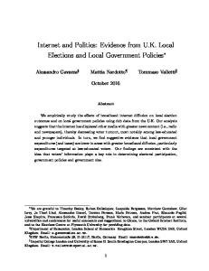
The aim of this paper is to estimate the causal effect of female representation in the State Legislatures, both in general and Scheduled Caste and Scheduled Tribe seats, on expenditure, public goods and different laws passed by the states in India. For this I use a dataset collected on state politicians in India during the period 1967-2000 which includes data on laws, public goods and expenditures. The electoral data have been collected from the electoral reports published by the Election Commission of India. From these reports information was gathered on individual candidates for the state elections in India from 1967-2001: their gender, political party, whether they contested for an SC/ST reserved seat or not, and for female candidates the votes they received and information about who were they running against. More details on the construction of the variables used in this study are shown in the data appendix. Figure 1 shows variation across election years and states of both SC/ST and general female representation. SC/ST and general female representation has been low in all states during the time period under consideration. In fact, between 1967 and 2001 at most 11% of the seats have been won by a general woman and 5% of the seats have been won by an SC/ST woman. 2

For a more precise definition of Scheduled Castes and Scheduled Tribes see Pande (2003).

6

Moreover, different states follow different trends in both general and SC/ST female political representation. [FIGURE 1 HERE] Table 1 shows descriptive statistics on the electoral variables used in this study. During this time period, 3.6% of the seats were won by women, 2.8% in general seats and 0.8% in SC/ST reserved seats. Despite the fact that female political representation is very low for all states in India, both general and SC/ST female representatives are shown to have an effect on policy decisions. Due to the way decisions are taken in the State Legislatures in India, even if female legislators do not constitute a "critical mass" in any voting procedure, they can still convince other legislators during or before the discussions, and they can also introduce proposals that are then voted by the legislature. Mishra (2000) presents evidence from the debates in the Orissa Legislative Assembly showing that female legislators introduce proposals in the legislature, participate in the debates and try to convince their male counterparts of their ideas. This is true for both general and SC/ST female legislators. [TABLE 1 HERE] In order to have a broader view of the effects of female representation, I use as dependent variables laws, educational inputs, public goods and budget expenditures. To obtain direct evidence on whether female politicians favour women and the poor in policymaking, two measures of laws enacted are used: one serving the interests of the poor and the other serving women’s interests. For the first one I use the cumulative number of land reforms designed to tackle poverty enacted by the different states in India during 1968-1992. The types of land reforms used are Tenancy Reforms, Abolition of Intermediaries reforms and Land Ceiling legislation3 . The "women-friendly" policy variable used is a dummy variable which equals one the year a given state has made an amendment to the Hindu Succession law, with data taken from 1968-2000. These amendments are designed to ensure that both women and men have the same inheritance rights. Then I analyze the effect of female representation on some educational inputs and public goods measures. For educational inputs I use the number of teachers per 1000 individuals in primary, middle and secondary institutions, together with the fraction of female teachers in each type of institution. In addition I use information on the number of secondary, middle, 3

I use the land reform measure created by Besley and Burgess (2000). Details on this variable can be found there.

7

and primary schools per every thousand individuals. This will give an approximate idea of the supply of education. I also use data on other public goods measures, such the number of hospitals, dispensaries and beds in hospitals and dispensaries per every 1000 individuals. This will give information on health provisions. Descriptive statistics for all these variables are shown in Table 2. [TABLE 2 HERE] Finally, I analyse the impact of female legislators on different components of the state budget. For this I have collected data on actual Revenue and Capital expenditure for each state and year. All the states in India use the same budgetary classification, so expenditures from different states can be safely compared. Revenue expenditure is defined as expenditure on current consumption of goods and services of the departments of Government, expenditure on Legislature, State Administration, tax collection, debt servicing, interest payments and grants-in-aid to various institutions. Capital expenditure is defined as expenditure devoted to acquiring or creating assets of a material and permanent nature or to reduce liabilities. Revenue expenditure in each one of the state’s budgets is divided among two main categories: Development expenditure and Non-Development expenditure. Development expenditure is money allocated to the maintenance of capital assets, both economic and social. Non-Development expenditure is directed towards current and consumption expenditures of the government. Total Capital Disbursements are divided into two main categories: Total Capital Outlay and Discharge of Internal Debt. Total Capital Outlay is mainly composed of Development expenditure, which includes both Social and Economic Services. Discharge of Internal Debt includes different types of loans. Figure 2 shows graphically how all the different expenditure categories are organized in both the capital and the revenue budgets in all the Indian states. The larger expenditure categories for which there were enough observations in both the capital and revenue budgets are selected, and capital and revenue expenditures are aggregated for each one. I then use the share of Total Expenditure devoted to each type of expenditure as an expenditure measure. This measure can be used to understand whether female politicians have an effect on the overall budget allocation. Descriptive statistics for the expenditure variables appear in Table 2. A budget reclassification took place in 1972, which means that budget data for the period 1967-1972 cannot be safely compared for all the expenditure categories to 8

budget data from later periods. For this reason I focus on the time period 1972-2000 for the expenditure variables. The nominal variables are deflated using the Consumer Price Index for Agricultural Labourers (CPIAL) and the Consumer Price Index for Industrial Workers (CPIIW). The reference period used is October 1973-March 1974. [FIGURE 2 HERE]

3

Empirical Strategy

To analyse the effects of having female representation in both SC/ST and general seats in the State Assemblies on government expenditure, public goods and laws enacted, I use panel data for the 16 main states in India during the period 1968-2000. The main difficulty is to assess the causal effect of female representation on the different policy outcomes. To illustrate this, assume that the first empirical specification to be tested is:

Yit = αi + β t + γFit + Xit δ + uit

(1)

Where Yit is the measure of expenditure, public goods or policy for state i in year t. αi and β t are state and year fixed effects, Fit is the fraction of seats occupied by women in the state assemblies4 as elected in the previous elections, and Xit stands for other control variables included in the regression which vary across state and over time and can also have an effect on the dependent variables of interest. Even though state fixed effects control for permanent differences across states in female representation and the outcome variables, and year fixed effects control for nationwide shocks in female representation and the outcome variables, I cannot rule out the existence of an omitted variable that varies across states and over time and affects both female representation and the outcome variables. Thus, the OLS estimates reported in this econometric specification would be biased, and specification 1 would not allow the effect of female representation on the dependent variables of interest to be correctly identified. The same identification challenge is faced when dividing female politicians according to whether they contested for an SC/ST reserved seat or not: 4

If each legislator has one vote, the fraction of legislators that are female will respresent the weight that female politicians have in the legislature.

9

Yit = αi + β t + ϕF genit + θF scstit + Xit δ + uit

(2)

Where F genit is the fraction of seats won by general women as elected in the previous elections and F scstit is the fraction of seats won by SC/ST women as elected in the previous elections. As before, the omitted variable could affect the dependent variable and be correlated with the fraction of seats in the state won by general and SC/ST female politicians. To be clear, if women are elected in constituencies where there is a “preference for female politicians”, this variable will affect how many general and SC/ST female legislators are elected, thus, biasing the results obtained.

3.1

Identification Strategy

In order to identify the causal effect of female politicians, what is needed is an exogenous variation on who ultimately wins the seat. For this, I take advantage of the existence of close elections between a female and a male candidate, elections in which the winner beat the runner up by a very small number of votes5 . As an instrument for the fraction of seats won by a female politician I use the fraction of seats won by a female politician in a close election against a male politician. Female candidates who barely won the elections against a man do so in constituencies where there is no clear "preference for female politicians", and are ex-ante comparable to constituencies in which male candidates win by a very small margin of votes against female candidates. In very close elections, if there is an element of uncertainty about the final outcome, the winner will be determined by chance (turnout, or other elements related to the election day). Then, in elections in which the first two candidates are of different genders, either the female or the male candidates could have won the election and, thus, the fact that the female candidate won the seat instead of the male can be considered as good as random. I instrument the fraction of seats won by female politicians, with the fraction of seats won by female politicians who won "by chance", or due to this randomness. Having controlled for the fraction of seats in the state that had close elections between 5

Close elections are defined as those in which the winner beat the runner up by less than 3.5% of votes. In the robustness checks section I run the regressions in which close elections are defined by different margins and results do not change.

10

female and male candidates in both stages, the exclusion restriction is satisfied, as the existence of close elections between women and men in a given state and year may not be a random event. However, the outcome of a close election can be considered as good as random, and since I consider close elections between a male and a female candidate, the gender of the winner can also be considered as good as random. Thus, the fact that there have been close elections between a female and a male candidate generates "near-experimental" causal estimates of the effect that female political representation has on the policy variables. The first stage regression is:

Fit = αi + β t + κF Cit + µT Cit + Xit δ + εit

(3)

Fit is the fraction of seats in the state that were won by a female politician as elected in the previous elections. The instrument for this variable is F Cit , the fraction of seats in the state won by a woman in a close election against a man. In order to construct the instrument I use data on the vote share received by each one of the female candidates in state elections in India during then period 1967-1999, together with the margins of votes obtained against the winner or, in the case they won the elections, data on the runners-up and the margin of votes obtained against them. For the election years I use female representation as it was in the previous elections, under the assumption that newly elected legislators may not have much power during the first year6 . Moreover, this controls for the fact that some of the elections are held at the end of the year, when decisions have already taken place. The year fixed effects control for nationwide shocks or policies that were implemented in all states at the same time. The state fixed effects control for state specific characteristics that do not vary over time. The second stage regression is specification 4, Yit is the policy outcome variable for state i at time t. Since observations in the same state and electoral cycle could be correlated, I compute the robust standard errors clustered at the state and electoral cycle7 .

Yit = αi + β t + γFit + λT Cit + Xit δ + uit

(4)

I control for T Cit , the fraction of seats in the state in which there were close elections 6

Results are robust to including the contemporaneous female representation variable in the election years. This is available from the author on request. 7 I cannot cluster at the state level as I only have included 16 states in the sample.

11

between women and men in both stages. The fraction of seats that had close elections between men and women controls for the fact that the existence of this type of close election may not be a random event. However, the outcome of a close election can be considered as good as random, meaning that the winner’s gender in close elections between women and men can be considered as good as random as well. To be clear, the impact of the existence of close elections between women and men on the policy variables should be controlled for in specification 4 and partialled out of the instrument in specification 3. To identify the effects of female politicians who contested for SC/ST seats separately from the effect of female politicians who contested for general seats, a similar strategy is used, but I now take advantage of the fact that some seats in the State Assemblies are reserved for the Scheduled Castes and Tribes. I then divide the female representation variable according to whether female politicians were contesting in an SC/ST reserved seat or not. The reason behind dividing female representatives is that female legislators who won the election for a general seat might have different policy preferences than female legislators who won the election for an SC/ST seat. India provides the opportunity of exploiting mandated political reservation for SC/STs to divide the female representation variable according to the type of seat for which they contested. The comparison of SC/ST and general female legislators provides evidence on whether the identity of the legislator is defined by both gender and caste, allowing the distinction between gender and caste effects. If the cost of running for election is higher for women than for men, female legislators will be of comparatively higher classes than men legislators. Thus, the female representation variable may only indicate class, not gender. This will not be the case for SC/ST female legislators, as they come from the poorest section of the society. I instrument the fraction of seats won by SC/ST female politicians by the fraction of seats won by SC/ST women in a close election against an SC/ST man, defining close elections in the same way as before8 . Similarly, I instrument the fraction of seats won by a general woman by the fraction of seats won by a general woman in a close election against a general man. I then estimate a first stage regression similar to 3 separately for SC/ST and general female politicians and a second stage regression of the form: 8

There has almost never been a case in which an SC/ST legislator won a non-reserved seat. This implies that knowing whether a seat is reserved or not, one can know the caste of the legislator who wins that seat.

12

Yit = αi + β t + ϕF genit + θF scstit + λT Cit + Xit δ + uit

(5)

In these regressions I also control for T Cit in both stages, as the existence of close elections cannot be considered a random event. In all regressions I include as control variables the proportion of seats won by each one of the parties in each election, in order to distinguish the effect of gender from the effect of party ideology9 . Other control variables include the real net state domestic product per capita, the share of rural population over total population, and a dummy for the year before the elections took place. All these variables could affect the dependent variable in different ways: the rural population variable and the real net state domestic product per capita could give an idea of the economic backwardness of the state, which can also influence the policy decisions adopted. The dummy variable for the year before the elections takes into account that legislators might adopt different policies just before elections, in order to increase their probability of being re-elected. Other controls are the fraction of seats reserved for SC/STs as this can also affect the type of policies applied. As reservation for lower castes is a function of the SC/ST population, it is also controlled for in the regressions. I also include state-specific time trends in the regressions. The identification strategy is based on the regression discontinuity design, although it is not directly used in this study. To do this, I would need to relate each particular legislator to a policy decision, and decisions are taken by the whole legislature. Since in India, State Assemblies are composed by many legislators who choose a single expenditure measure or policy each year, I used close elections as an instrument. Regression discontinuity has been widely used and was first introduced in the context of elections by Lee (2001) for incumbency advantage and Pettersson-Lidbom (2001) for the effect of party control on fiscal policies. Regression discontinuity has been used as an instrument by Angrist and Lavy (1999) to estimate the impact of class size on educational achievements and by Rehavi (2003), who used close 9

There are eight main party groups: Congress, Hard Left, Soft Left, Janata, Hindu, Regional, Independent candidates and other parties. Congress parties include Indian National Congree Urs, Indian National Congress Socialist Parties and Indian National Congress. Hard Left parties include the Communist Party of India and Communist Party of India Marxist. Soft Left parties include Praja Socialist Party and Socialist Party. Janata parties include Janata, Lok Dal, and Janata Dal parties. Hindu parties include the Bharatiya Janata Party. Regional parties include Telegu Desam, Asom Gana Parishad, Jammu & Kashmir National Congress, Shiv Sena, Uktal Congress, Shiromani Alkali Dal and other state specific parties.

13

elections between women and men in the US as an instrument to estimate the effect of female politicians at the state level on expenditures. In the same spirit, to identify the causal effect of female politicians I use as an instrument for female representation the fraction of seats in the state won by a woman in a close election against a man.

3.2

Validity of the Identification Strategy

To identify the effect of female politicians, both in aggregate and for general and SC/ST seats I take advantage of the fact that some of these female politicians won in close elections against men. For this to be a valid identification strategy, one should show that the fraction of close elections won by women in a given state and year cannot be predicted by any other state characteristic. This is done in Table 3. I have tried to predict the fraction of close elections between women and men won by women per state and election year. This is done for all seats, and then separately for SC/ST reserved seats and for unreserved seats. I run a regression with these variables as dependent variables and different state characteristics on the right hand side, controlling for state and year fixed effects. Even though this is not proof of exogeneity, reassuringly, variables such as electoral turnout, the proportion of seats in close elections contested by the different parties, the proportion of reserved seats, political competition10 , the proportion of seats that had close elections in the past, the proportion of seats won by women in the past and literacy rates do not have any effect on the fraction of close elections between women and men won by women. [TABLE 3 HERE] In addition, if the outcome of a close election is to be considered random, it should be observed that states and electoral years in which more men than women won in close elections have similar characteristics as compared to states and electoral years in which more women than men won. In other words, both types of states and years should only differ in the fraction of close elections won by female politicians. In Table 4 different characteristics are compared for both types of states and years for three cases, those in which more men/women won, those in which more SC/ST men/women won and those in which more general men/women won. I report the difference between the mean of each variable for both groups, together with the 10

Political competition is defined as minus the absolute value of the absolute difference in the share of seats occupied by the dominant political party and its main competitor. See Besley and Burgess (2002).

14

corresponding standard error. I use information on the proportion of seats won by female politicians in elections that were not close, the number of female candidates per seat, male and female turnout, the proportion of reserved seats, newspaper circulation per capita and real net state domestic product. None of the differences are significant and they are all very small. [TABLE 4 HERE] Identification comes from variation across states and years in the proportion of seats won by women in a close election against a man, having controlled for the fraction of seats that had close elections between women and men. In order to derive policy implications from the results obtained, it is useful to check that states and electoral years which had more close elections between women and men do not have different characteristics than the rest. In Table 5, I compare different characteristics for states and years which had more or fewer close elections than the median. I use information on the fraction of urban population, male and female literacy rates, the fraction of seats that are reserved for SC/STs, male and female turnout, newspaper circulation per capita and the proportion of seats won by the different political parties. Given that both types of states and electoral years are very similar in those characteristics, I can argue in favour of the external validity of the results obtained11 . [TABLE 5 HERE] Finally, candidate and constituency characteristics should be very similar as well, whether female or male candidates won the election. This is shown in Table 6. Male and female candidates who won in close elections against a candidate of the other gender did so in constituencies where there were the same number of female candidates, where the winner was the incumbent the same number of times, in constituencies that had the same number of close elections in the past, and where turnout was the same and the winner received the same number of votes. This happens for all seats, for general seats and for SC/ST reserved seats. Interestingly, the winner receives around 40% of the votes, while the runner up receives more than 36.5% of the votes; this leaves any other potential candidates with 23.5% of the votes, which is a large difference between the winner and the runner up. [TABLE 6 HERE] 11

It is important to still include the fraction of seats won in close elections between women and men in both stages in the 2SLS, as the test in Table 5 does not take into account intertemporal variation.

15

4

Results

4.1

Laws

As a first step, in this section I explore the effects of having female representation in the State Assemblies in India in two types of policies, one which is directly targeted to women and another one which targets the poor. The different states in India have had the power to amend different national laws and to implement different types of land reforms during the time period under consideration. The first policy to be analyzed directly favours women, as it gives them inheritance rights. The Hindu Succession Act (1956) deals with intestate succession among Hindus12 . It includes the concept of the Mitakshara Joint Family, under which on birth, the son acquires a right and interest in the family property. According to this, a son, grandson and great grandson constitute a class of coparcenaries, based on birth in the family. Under this system, joint family property devolves by survivorship within the coparcenary, but no female is a member of the coparcenary. During the time period under consideration, five states in India have recognized that a daughter needs to be treated equally and become a coparcener in her own right in the same way as the son. The state of Kerala in 1975 abolished the right to claim any interest in any property belonging to an ancestor during his or her lifetime. They abolished the Joint Hindu Family system, solving the gender differentials in inheritance rights13 . The other four states, namely Andhra Pradesh, Tamil Nadu, Maharashtra and Karnataka amended the Hindu Succession law by removing the gender discrimination in the Mitakshara Coparcenary system14 . A variable is created which is equal to one if the state has legislated in favour of the abolition of gender discrimination in that particular year or in the past and zero otherwise. The second policy to be analyzed benefits the poor. Land reforms can be considered redistributive policies, aimed at improving the poor’s access to land in developing countries. 12

Hindus constitute approximately 80% of the population in India. However, this law applies to anyone who is not a Muslim, Christian, Parsi or Jew by religion. 13 The Kerala Joint Family System (Abolition) Act, 1975. 14 The Hindu Succession (Andhra Pradesh Amendment) Act 1986. The Hindu Succession (Tamil Nadu Amendment) Act 1989. The Hindu Succession (Maharashtra Amendment) Act 1994. The Hindu Succession (Karnataka Amendment) Act 1994. The Hindu Succession Act was further amended in 2005 to give women equal inheritance rights as men. However, 2005 is not included in the time period studied here.

16

Besley and Burgess (2000) classify land reform acts into four main categories according to the purpose they were designed for. The first category is called Tenancy Reform, which regulates tenancy contracts and attempts to transfer ownership to tenants. The second category of land reforms consists of attempts to abolish intermediaries. Intermediaries worked under feudal lords and collected rents for the British. They were known for extracting high rents from the tenants. The third category of land reforms implements ceilings on land holdings. The fourth category of land reforms was designed to allow consolidation of disparate land-holdings. In this study I use a cumulative measure of the first three types of land reforms, which were the ones primarily designed to tackle poverty. The variable used is equal to the sum of the cumulative number of land reform acts in each category passed in the state. Results for these policies are reported in Table 7. Columns 1, 2, 5, and 6 contain results for the OLS regressions, while columns 3, 4, 7 and 8 give results for the 2SLS regressions. OLS results do not show any effect of female political representation, whether considered in aggregate or dividing female legislators according to whether they contested in an SC/ST reserved seat or not, nor for the Hindu Succession Law (columns 1 and 2), or the Land Reforms (columns 5 and 6). However, as discussed before, OLS results can be contaminated by omitted variable bias. 2SLS results give a different picture. Results for the Hindu Succession Law are reported in columns 3 and 4 of this table. In this case women representatives do not have any impact on these amendments when considered in aggregate. In contrast, when dividing the female representation variable according to whether they contested for an SC/ST reserved seat or not, only SC/ST women legislators have a positive and significant effect on this variable. Surprisingly, general female legislators do not have an effect on this variable. The fact that no effect is found for general female legislators might be due to their class position. In fact, elite women will be less likely to favour women-friendly policies if class and gender effects go in opposite directions. Low caste women, since reservations are already made for SC/ST people, will be more likely to perceive themselves as representatives for women as well as representatives for the Scheduled Castes and Scheduled Tribes. [TABLE 7 HERE] Results for land reforms give a more precise idea of the importance of caste as well as gender in determining policy. While female politicians do not have a significant effect on land reforms, once SC/ST and general women legislators are considered separately in the 17

regressions, general female legislators have a negative and significant effect on land reforms while SC/ST have a positive and significant effect; see columns 7 and 8. This is consistent with the fact that general women legislators may be part of the elite and will then oppose these reforms. Given that SC/STs are poorer, results obtained for land reforms clearly reflect the caste effect. The 2SLS coefficients are very different in magnitude from the OLS ones, especially for SC/ST female legislators. This could indicate that SC/ST female legislators are elected where more laws benefiting women and the poor are needed. First stage regressions are reported in Table 8 for both samples; the fraction of female legislators that won in a close election against a man is a strong predictor of the fraction of seats in the state won by a woman. This is also true when dividing the female representation variable according to whether the female legislator contested for an SC/ST reserved seat. [TABLE 8 HERE] Taken together, these results point to the fact that the identity of the legislator influences policy decisions, but that both gender and caste should be taken into account, as there may be important class differences by gender that could determine the preferences of the legislators and, as a consequence, the policies applied. The reference category here is men, meaning that SC/ST female legislators increase the amount of pro-women and pro-poor legislation more than men, and general female legislators decrease the amount of pro-poor legislation more than men. However, the coefficients for SC/ST and general female legislators are also significantly different from one another15 , proving that caste as well as gender matters.

4.2

Education

The second set of variables used to identify whether male and female legislators have different policy preferences are education variables. In this section I look at the effect of female representatives on certain educational input measures, in order to analyse their impact on the supply of education. Educational policies are mainly decided by the state governments, so it is interesting to analyze whether female representation at the state level increases the amount of educational inputs provided. Given that it has been documented in the literature that women tend to support child related expenditures more than men, it is as well interesting to analyze whether female politicians invest in education more than men. In addition, given that SC/STs 15

This is available from the author on request.

18

individuals have had difficulties accessing education, caste should also be taken into account. I first use the number of primary, middle and secondary schools per thousand individuals. Results are shown in Panel A of Table 9, while first stages for all samples used in these regressions are shown in Panel B. OLS results are shown in columns 1 and 2 (primary schools), 5 and 6 (middle schools) and 9 and 10 (secondary schools).These results could be contaminated by omitted variable bias, but they show that female representatives are positively correlated with the number of middle schools per thousand individuals, but not with the number of primary and secondary schools. While SC/ST female politicians are positively correlated with the number of secondary schools, general female politicians are only positively correlated with the number of middle schools. Results for the corresponding 2SLS regressions are reported in columns 3 and 4 (primary schools), 7 and 8 (middle schools) and 11 and 12 (secondary schools). Results are quite different, and the difference between the 2SLS and the OLS coefficients is positive in all cases, which could indicate that female politicians are elected where more education is needed, or where there are fewer educational inputs16 . In fact, results show that female political representation has a positive effect on the number of primary, middle and secondary schools per thousand individuals. The largest effect is found in primary schools, even if the coefficient is only significant at the 10% level. When dividing the female representation variable according to whether the female politicians contested for an SC/ST seat or not, SC/ST female politicians have a positive effect on primary and secondary schools, while general female politicians increase the number of middle and secondary schools. By increasing SC/ST female representation by 1 percentage point17 , the number of primary schools per 1000 individuals increases by 0.03 units, which is 4% of the average. Their coefficient for secondary schools is smaller, but by increasing female representation by 1 percentage point, the number of schools per 1000 individuals increases by 0.004 units, which is also 4% of the average. By increasing general female representation by 1 percentage point, the number of middle and secondary schools increase by 0.003 and 0.0014 units per 1000 individuals, which is 1.5% and 1.4% of the average respectively. [TABLE 9 HERE] As another educational input, I use the number of teachers per 1000 individuals in each 16 17

As before, this is especially true for SC/ST female politicians. The standard deviation is 0.09, see Table 1.

19

type of schools. Results are shown in Panel A of Table 10. OLS results are shown in columns 1 and 2 (primary), 5 and 6 (middle) and 9 and 10 (secondary). Results for the corresponding 2SLS regressions are reported in columns 3 and 4 (primary), 7 and 8 (middle) and 11 and 12 (secondary). First stages for these regressions are the same as those reported in Table 9. As another educational input, I use the number of teachers per 1000 individuals in each type of schools. Results are shown in Panel A of Table 10. OLS results are shown in columns 1 and 2 (primary), 5 and 6 (middle) and 9 and 10 (secondary). Results for the corresponding 2SLS regressions are reported in columns 3 and 4 (primary), 7 and 8 (middle) and 11 and 12 (secondary). First stages for these regressions are the same as those reported in Table 9. Results for the 2SLS specifications show no effect of female politicians on the number of teachers, this holds for the three education tiers. However, having divided the female representation variable according to whether the female politicians contested for an SC/ST reserved seat or not, SC/ST female politicians increase the number of teachers per 1000 individuals in primary education and decrease it in middle education. In contrast, general female politicians do not have any effect in any of the tiers. [TABLE 10 HERE ] Finally, I analyse the impact of female politicians on the fraction of teachers that are female in primary, middle and secondary schools. There is some evidence that the presence of female teachers may encourage girls to go to school, thus, it is interesting to understand whether female politicians have had any impact on the number of female teachers per each type of schools. Results are provided in Panel B of Table 1018 . 2SLS results suggest that female politicians increase the proportion of teachers that are female in primary schools; in fact, a 1 percentage point increase in female representation increases the proportion of teachers that are female by 0.013, which is around 5% of the average. However, no results are found for teachers in middle and secondary schools. Having considered SC/ST and general female politicians separately, SC/ST female politicians increase the fraction of teachers that are women in primary education, while general female politicians increase the fraction of teachers that are women in secondary education. Taken together, these results show that female politicians increase the number of schools in all education tiers and increase the proportion of teachers that are female in primary education. 18

First stage regressions are those in Table 9.

20

However, once they have been divided according to whether they were contesting for an SC/ST reserved seat or not, SC/ST female legislators seem to put more emphasis on lower levels of education than general female legislators do. In fact, their effect on primary education is always significantly different from the effect of general female legislators on primary education19 . The fact that only SC/ST female legislators have an effect on primary education can be explained by the fact that SC/ST individuals, especially SC/ST women, have less access to education, so they will be more likely invest in lower tiers of education. In contrast, general women have more access to higher tiers of education, and thus they invest in middle and secondary schools once in politics.

4.3

Health

Results obtained so far show that the identity of the legislator is indeed defined by gender and caste, as general and SC/ST female politicians choose different policies. Moreover, results suggest that they choose policies that may benefit their groups more. However, it is also interesting to see whether female politicians also favour investment in other public goods, like those related to health provision. Health in India is a very important welfare issue for which the preferences of male and female politicians could differ. I use information on the number of hospitals, dispensaries and beds in hospitals, and dispensaries per thousand individuals to get an idea of their effect on health provision. Results are shown in Panel A of Table 11. First stage regressions for each of the three samples are shown in Panel B. Female politicians do not have any differential effect compared to men on hospitals and dispensaries; in contrast, by increasing female representation by one percentage point, the number of beds in hospitals and dispensaries increases by 0.034, which is 4.4% of the average. When dividing the female representation variable in columns 4, 8, and 12 neither SC/ST nor general female politicians have a different effect from men on hospitals. However, SC/ST female politicians do have an impact on the number of dispensaries, even if the coefficient is only significant at the 10% level, and they are the ones who most increase the number of beds in hospitals and dispensaries. General female politicians also increase the number of beds in hospitals and dispensaries but their effect is 3.4 times smaller and the two coefficients are 19

Available from the author on request. This is true for schools, teachers and the fraction of teachers that are female.

21

significantly different. [TABLE 11 HERE] Results suggest that female politicians, and specifically SC/ST female politicians, increase health provisions. Even though they do not have an effect on hospitals or dispensaries, beds in hospitals and dispensaries may be a better measure of the health-related public goods provided; as with the other measures one does not take the size of the hospitals and dispensaries into account.

4.4

Expenditure

Results show that female politicians have an impact on investment in public goods and laws approved in India. Moreover, whether they contested for an SC/ST reserved seat or not should also be taken into account. In this section, I analyse the impact of female representation on the composition of total expenditure in the state budgets in India. In each one of the states, the budget is approved by the legislature after the enactment of what is called the Appropriation Act, which gives authority to the government to withdraw money from the Consolidated Fund20 . Usually a budget speech is given to the legislature by the Finance Minister of each state, and two days later there is a general discussion in the legislature about the budget proposal presented. This discussion lasts 6 days. After that, and during a maximum period of 18 days, individual demands made by the individual legislators are voted in the Legislative Assembly. Then, the introduction, consideration and passing of the Appropriation Bill in the Legislative Assembly with the Governor’s consent lasts for about two days. In total, the budget discussion takes a maximum of 26 days. Table 12 shows results for the main expenditure classifications. Columns 1-6 show results for the female representation variable, while columns 7-12 show the results obtained when the female representation variable is divided according to caste. In column 1 results are given for the logarithm of total expenditure per capita; in this case the coefficient for the proportion of seats in the state won by female politicians is very close to zero and not significant. This indicates that female politicians did not increase the size of the government. Column 2 gives results for the fraction of total expenditure devoted to capital investments; as before, the 20

Defined by the Constitution as “all revenues received by Government, all loans raised by Government by issue of treasury bills, loans or ways and means advances and all money received by Government in repayment of loans”.

22

coefficient obtained is not significant. This means that female politicians do not have an effect on how expenditure is divided among the revenue and capital budgets. It is now interesting to analyze whether they affected the actual composition of expenditure, after aggregating the revenue and capital budgets for each of the categories. Both capital and revenue expenditure can be divided into two broad categories: Development expenditure and Non-Development expenditure. Results for these categories are shown in columns 3 and 4. Female politicians have a positive effect on non-development expenditure, but the effect on development expenditure is not significant. Development expenditure can be further divided into Economic and Social expenditure. Results for these two categories are given in columns 5 and 6. Female political representation does not have any effect on Social Expenditure but it does increase the fraction of the budget devoted to Economic expenditure. Columns 7-12 show results for the same variables. The difference is that I then report coefficients for the fraction of seats in the state won by SC/ST female politicians and general female politicians. Neither SC/ST nor general female politicians have an effect on the log of per capita total expenditure or the fraction of total expenditure spent on capital expenditures. SC/ST female politicians have a positive effect both on Development expenditure and on NonDevelopment expenditure; see columns 9 and 10, this means that they reduce expenditure on loans given or repaid. In contrast, general female politicians do not have any impact on these two expenditures categories. Results in columns 11 and 12 show that SC/ST female politicians do not have an effect on Social and Economic expenditure. However, general female politicians decrease Social expenditure while increasing Economic expenditure. A one percentage point increase in general female representation decreases Social expenditure by 0.5 percentage points and increases Economic expenditure by 0.9 percentage points. This further confirms the fact that, given that general female politicians may belong to higher classes, they will be inclined to spend less on social issues, and more on economic issues. [TABLE 12 HERE] It is also interesting to understand whether female representation has had an impact on smaller expenditure categories within Social and Economic expenditure. Results are reported in Table 13. Panel A shows results for the fraction of seats in the state won by a female politician. In Panel B the female representation variable is divided according to whether 23

the female politicians contested for an SC/ST reserved seat or not. Results are reported for five categories within Social expenditure: Education, Health, Family Welfare, Housing and Social Security. Results are also given for 3 categories within economic expenditure: agriculture, industry and minerals and general economic services21 . Results in Panel A show that female politicians only have an effect on two of the categories: Housing expenditure, which they reduce, and industry and minerals, which they increase. Results in Panel B show that SC/ST female politicians only have an effect in two expenditure headings: they decrease Social Security and Welfare and they increase General Economic Services. General female politicians only have an effect on the fraction of total expenditure devoted to Housing, which they reduce as well. [TABLE 13 HERE] Even if female politicians have an effect on educational and health inputs, they do not have much of an impact on the allocation of budget expenditures, and they do not seem to have an effect on the fraction of total expenditure devoted to Health and Education. This is not surprising if we take into account that these expenditure headings may be too broad and what ultimately matters is how each one of the expenditure headings is spent. In addition, female politicians will have an impact on these expenditures if their preferred levels of expenditure are different from the actual ones, otherwise they may be more interested in deciding how the money is spent within each one of the headings. The fact that SC/ST female politicians reduce Social Security and Welfare is surprising, but it may be due to the fact that lower castes do not benefit much from it.

5

Robustness Checks

In this section I perform some robustness checks to support the validity of the main results obtained. In the main specifications, close elections are defined as elections in which the vote difference between the winner and the runner-up is less than 3.5%. Here I check whether results are sensitive to this choice of vote margin. In Panel A of Table 14, I test whether results are the same when close elections are defined as those in which the winner beat the runner-up by different margins: 4%, 3% and 2.5%. Then the 2SLS specification is run as before. Now, 21

For the other categories the sample size was too small.

24

however, the instrument will be defined in a different way, because some elections that were considered close before will not be considered now as such. I only report the coefficients for the fraction of seats won by female politicians corresponding to specification 4 and the coefficients for the fraction of seats won by SC/ST and general female politicians corresponding to specification 5. Throughout, results remain mainly unchanged, even though some coefficients increase when the margin of close elections is reduced22 . This paper shows that both gender and caste should be taken into account when defining the identity of the legislator, however, the caste results rely on the reservation of some seats in the state governments for the SC/STs. Similar to Pande (2003), and since SC/ST reservation is a nonlinear function of SC/ST population, I include as controls the proportion of the population that was SC/ST according to the previous census as well as its square, cube and quartic in the regressions. Results are shown in Panel B of Table 14. I first add the SC/ST proportion according to the previous census and results are very similar to those obtained before, then I add the square, the cube and the quartic and, reassuringly, results remain unchanged.

6

Conclusions

This paper shows that female legislators have different effects on expenditure, public goods and policy decisions than their male counterparts. Moreover, whether these female legislators belong to scheduled castes/tribes or won the elections for general seats also matters for policy determination. Scheduled Caste and Scheduled Tribe female legislators favour investments in primary education more than men and more than general female legislators. They also favour more investments in beds in hospitals and dispensaries. They favour development expenditure, "women-friendly" laws, such as amendments to the Hindu Succession Act, proposed to give women the same inheritance rights as men. They also favour pro-poor redistributive policies such as land reforms. In contrast, general female legislators do not have any impact on "women-friendly" laws, they oppose redistributive policies such as land reforms, invest in 22

This points to the fact that the identification strategy used in this paper obtains variation from those states and years in which women and men contested in close elections and perhaps the degree of electoral competition in these elections draws candidates who, in equilibrium, have preferences that differ more by gender than in other types of elections.

25

higher tiers of education and reduce social expenditure. In order to interpret these results, one must take into consideration the class of these legislators, as well as gender. Given the difficulties faced by women trying to enter political life, female legislators may tend to belong to higher social classes than male legislators. This is especially the case for general female legislators, given that Schedule Caste/Tribe female legislators will have lower economic backgrounds. If general female legislators belong to a comparatively higher class than general male legislators, results for these legislators may be such that they capture more the "class" than the gender effect. However, this will not be the case for SC/ST female legislators, for whom the gender effect can indeed be captured by results in this paper. SC/ST female legislators favour land reforms and women-friendly laws, they also invest more on health than general female legislators. These results seem to indicate that SC/ST female legislators identify themselves with women, especially the poor and disadvantaged ones when taking their decisions. Moreover, low caste female legislators invest in primary education. Given the historical difficulties that low caste women have had to access education, they will be more likely to benefit from this type of education than from middle and secondary education. However, unlike results for SC/ST female legislators, results for general female legislators are somewhat different than findings for the United States, where women politicians seem to care about social, and especially family, issues23 . By taking into account that general women legislators belong to the elite, i.e., they have higher income and better jobs than the average in the state and sometimes belong to a family of politicians (Mishra, R.C. (2000)), these results seem to be explained by the class of these legislators. Moreover, the fact that general female legislators favour investment in middle and secondary education is consistent with this hypothesis, since only relatively rich women will be likely to receive middle and secondary education. There is evidence from other countries that the gender of the legislator matters for policy determination. However, data from other countries does not provide the opportunity to control for the social position of the legislator, which may be correlated with gender. India provides the unique opportunity to take this issue into account, by taking advantage of caste reservations. There is evidence from India that reservations for women in local governments and the 23

To the best of my knowledge, no paper in the US literature takes into account the socio-economic position of women legislators.

26

lower castes in the states and local governments do influence policy determination. However, there is no evidence on the effects of female representation in the state governments on policy, nor is there evidence on the effects of gender representation by caste.

27

7

Data Appendix

Electoral data: Collected from different volumes of the Statistical Reports on the General Elections to the Legislative Assemblies. The election commission of India publishes one report for every election in each state. There is data at the constituency level for the 16 main states in India for elections held during 1967-2001. -Proportion of seats in the state won by women: defined as the total number of seats in which a woman won the election in the state divided by the total number of seats in the state. This variable is lagged one period. -Proportion of seats reserved for SC/ST in the state: defined as the total number of seats reserved for Scheduled Castes and Tribes in the state divided by the total number of seats. This variable is lagged one period. -Proportion of seats in the state won by SC/ST and general female politicians: defined as the total number of seats won by Scheduled Castes and Tribe female politicians divided by the total number of seats in the state or the total number of seats won by general female politicians divided by the total number of seats in the state. This variable is lagged one period. -Proportion of seats in the state won by women in a close election against a man: defined as the number of women in the state who won by less than 3.5% of votes against a man over the total number of seats in the state. This variable is then lagged one period. -Proportion of seats in the state in which a man and a woman contested in a close election: defined as the number of men and women in the state who won by less than 3.5% of votes against a candidate of the other gender over the total number of seats in the state. This variable is then lagged one period. -Proportion of seats in the state won by an SC/ST women in a close election against an SC/ST man: defined as the number of SC/ST women in the state who won by less than 3.5% of votes against an SC/ST man over the total number of seats in the state. This variable is then lagged one period. -Proportion of seats in the state won by general women in a close election against a general man: defined as the number of general women in the state who won by less than 3.5% of votes against a general man over the total number of seats in the state. This variable is then lagged one period. -Proportion of seats in the state won by each political party: number of seats won by the political party divided by total seats in the state. Congress parties include Indian National Congree Urs, Indian National Congress Socialist Parties and Indian National Congress. Hard Left parties include the Communist Party of India and Communist Party of India Marxist. Soft Left parties include Praja Socialist Party and Socialist Party. Janata parties include Janata, Lok Dal, and Janata Dal parties. Hindu parties include the Bharatiya Janata Party. Regional parties include Telegu Desam, Asom Gana Parishad, Jammu & Kashmir National Congress, Shiv Sena, Uktal Congress, Shiromani Alkali Dal and other state specific parties. Educational variables: From the publication “Education in India”. I am grateful to Tim Besley and Robin Burgess for sharing their data with me. -Data on schools: defined as the number of primary, middle and secondary schools in the state divided by the total population in 000’s. Data from 1968-1996 and from 1968-1992 for secondary education and for teachers. Variables have been interpolated where there were missing values. -Data on teachers: defined as the number of teachers in primary, middle and secondary school teachers in the state divided by the total population in 000’s. Also defined as the proportion of teachers that are female for each educational tier. Health: 28

Obtained from the Tim Besley and Robin Burgess database, I thank them for letting me use their data. -Hospitals: Variable defined as the total number of hospitals in the state divided by the total population in 000’s. Data from 1969-1998. Variables have been interpolated where there were missing values. -Beds in hospitals and dispensaries: Variable defined as the total number of beds in hospitals and dispensaries in the state divided by the total population in 000¡s. Data from 1971-1992. Variables have been interpolated where there were missing values. -Dispensaries: Variable defined as the total number of dispensaries in the state divided by the total population in 000’s. Data from 1969-1992. Variables have been interpolated where there were missing values. Expenditure: Collected from different monthly bulletins of the Reserve Bank of India. Some of the Revenue Expenditure data was updated from the Tim Besley and Robin Burgess database. Data from 1972-2000, even if it varies depending on the categories. Variables have been interpolated where there were missing values. -Data on Total expenditure: refers to Total Revenue Expenditure plus Total Capital Disbursements for every state and year. -Data on each one of the expenditure categories: refers to the total amount spent on the Capital budget plus the total amount spent on the Revenue budget in that particular category, divided by Total Expenditure. Public finance: Obtained from the Tim Besley and Robin Burgess database. -Data on Real Per Capita Net State Domestic Product: Net State Domestic Product deflated with the deflator described below and divided by the total population in the state. -Deflator: Consumer Price Index for Agricultural Labourers (CPIAL) and the Consumer Price Index for Industrial Workers (CPIIW). The reference period used is October 1973-March 1974 Laws -Land reforms: Obtained from the Tim Besley and Robin Burgess database. For more details refer to: http://sticerd.lse.ac.uk/eopp/research/indian.asp. Data from 1968-1992. -Hindu Succession Law: Obtained from: The Kerala Joint Family System (Abolition) Act, 1975, The Hindu Succession (Andhra Pradesh Amendment) Act 1986, The Hindu Succession (Tamil Nadu Amendment) Act 1989, The Hindu Succession (Maharashtra Amendment) Act 1994, The Hindu Succession (Karnataka Amendment) Act 1994. This variable is equal to one if there has been a “pro-women” amendment in the state and zero otherwise. Data from 1968-2000.

References [1] Ahluwalia, M.S., 2000. Economic Performance of States in Post-Reforms Period. Economic and Political Weekly, May 06-12. [2] Angrist, J.D. & Lavy, V., 1999. Using Maimonides’ Rule to Estimate the Effect of Class Size on Scholastic Achievement. Quarterly Journal of Economics. 114(2), 533-575. [3] Besley, T. & Burgess, R., 2000. Land Reform, Poverty and Growth: Evidence from India. Quarterly Journal of Economics, 105 (2), 389-430. [4] Besley,T. & Burgess, R., 2002. The Political Economy of Government Responsiveness: Theory and Evidence from India. Quarterly Journal of Economics, 117 (1), 1415-1452. 29

[5] Besley,T. & Burgess, R., 2004. Can Labor Regulation Hinder Economic Performance? Evidence from India. Quarterly Journal of Economics, 119(1),91-134. [6] Besley,T & Case,A., 2002. Political Institutions and Policy Choices: Evidence from the United States. Journal of Economic Literature, 41(1), 7-73.. [7] Besley, T. & Coate,S., 1997. An Economic Model of Representative Democracy. Quarterly Journal of Economics, 112(1)1), 85-114. [8] Besley,T. & Coate,S. , 2003. Elected versus Appointed Regulators: Theory and Evidence. Journal of the European Economics Association,1(5), 1176-1206. [9] Bose, S. & Singh, V.B., 1987-8. State elections in India: data handbook on Vidhan Sabha elections 1952-85. Vols. 1-5. New Delhi: Sage publications. [10] Case,A., 1998. The Effects of Stronger Child Support Enforcement of Non-Marital Fertility. In Irwin Garfinkel, Sara McLanahan, Daniel Meyer and Judith Seltzer (eds.) Fathers Under Fire: The Revolution in Child Support Enforcement, Russell Sage Foundation. [11] Chattopadhyay, R. & Duflo,E. , 2004. Women as Policy Makers: Evidence from a IndiaWide Randomized Policy Experiment. Econometrica, 72(5), 1409-1443. [12] Downs, A., 1957. An Economic Theory of Democracy. New York: Harper Collins. [13] Duflo, E., 2003. Grandmothers and Granddaughters: Old Age Pension and Intrahousehold Allocation in South Africa. World Bank Economic Review, 17(1), 1-25. [14] Edlund, L. & Pande, R., 2002. Why have Women become Left Wing? The Political Gender Gap and the Decline in Marriage. Quarterly Journal of Economics, 117, 917-961. [15] Edlund, L., Haider, L. , & Pande, R., 2005. Unmarried Parenthood and Redistributive Politics. Journal of the European Economics Association, 3 (2-3), 268-278 [16] Galanter, M., 1979. Compensatory Discrimination in Political Representation. A Preliminary Assessment of India’s Thirty-Year Experience with Reserved Seats in Legislatures. Economic and Political Weekly, issue 14. February [17] Government of India. National Perspective Plan for Women 1988-2000. [18] Lee D.S., 2001). The Electoral Advantage to Incumbency and Voter’s Valuation of Politician’s Experience: A Regression Discontinuity Analysis of Elections to the U.S. House. NBER working paper 8441. [19] Lee D.S. ,2008. Randomized Experiments from Non-Random Selection in U.S. House Elections. Journal of Econometrics.142(2), 675-697. [20] Lee D.S., Moretti E., & Butler, M.J., 2004. Do Voters Affect or Elect Policies? Evidence from the U.S. House. Quarterly Journal of Economics, 119(3),807-860. [21] Lott,JR & Kenny,LW., 1999. Did Women’s Suffrage Change the Size and Scope of the Government?. The Journal of Political Economy , 107, 1163-1198.. [22] Lundberg, S., Pollak, R., & Wales, T. ,1997. Do Husbands and Wives Pool Their Resources? Evidence from the Untied Kingdom Child Benefit. Journal of Human Resources, 32(3), 1132-1151. [23] Miguel, E. & Zaidi, F. , 2003. Do Politicians Reward their Supporters? Regression Discontinuity Evidence from Ghana. Mimeo, University of California, Berkeley. 30

[24] Mishra, R. C., 2000. Role of Women in Legislatures in India. A Study. Anmol Publications PVT. LTD. [25] Osborne, M.J. & Slivinski, A., 1996. A Model of Political Competition with CitizenCandidates. Quarterly Journal of Economics, 111(1), 65-96. [26] Pande, R., 2003. Can Mandated Political Representation Increase Policy Influence for Disadvantaged Minorities? Theory and Evidence from India. American Economic Review, 93(4), 1132-1151. [27] Pettersson-Lidbom, P., 2001. Do Parties Mater for Fiscal Policy Choices? A RegressionDiscontinuity Approach. Mimeo, Stockholm University. [28] Pettersson-Lidbom, P., 2008. Do Parties Mater for Fiscal Policy Choices? A RegressionDiscontinuity Approach. Journal of the European Economic Association, Volume 6, Issue 5, 1037—1056. [29] Rehavi, M., 2003. When Women Hold the Purse Strings: the Effects of Female State Legislators on US State Spending Priorities, 1978-2000. Mimeo. London School of Economics. [30] Sen, S., 2000. Toward a Feminist Politics? The Indian Women’s Movement in Historical Perspective. World Bank Publications. [31] Svaleryd, H., 2002. Female Representation-Is it Important for Policy Decisions?. Mimeo, Stockholm University. [32] Thomas, D., 1990. Intra-household resource allocation: an inferential approach. Journal of Human Resources, 25(4) 635-664. [33] Thomas,S., 1991. The impact of Women on State Legislative Policies. The Journal of Politics, 53(4), 958-976. [34] Thomas, S. & Welch, S. ,1991. The Impact of Gender on Activities and Priorities of State Legislators. Western Political Quarterly, 44(2), 445-446. [35] Thomas, S. ,1994. How Women Legislate. New York: Oxford University Press.

31

Assam

Bihar

Gujarat

Haryana

Jammu&Kashmir

Karnataka

Kerala

Madhya Pradesh

Maharashtra

Orissa

Punjab

Rajasthan

Tamil Nadu

Uttar Pradesh

West Bengal

0

.05 .1

0

.05 .1

0

.05 .1

0

.05 .1

Andhra Pradesh

1970

1980

1990

2000

1970

1980

1990

2000

1970

1980

1990

2000

1970

1980

1990

2000

year SC/ST female representation

General female representation

Figure 1: SC/ST and General Female Representation

Revenue Expenditure

Development

Social

Non-Development

Economic

Organs State State Administration

Education

Gen. Economic Serv.

Health

Agriculture

Labour welfare

Industry Minerals

Social Sec. W elf

Transport Communications

W elfare SC/ST

W ater Power Devel.

Police Public W orks

Housing W ater Supply San.

Total Capital Disbursements

Capital Outlay

Development

Social

Education Housing Health W elfare SC/ST Social Sec. W elf W ater Supply San.

Loans repayed/given

Non-Development

Economic

Agriculture Industry Minerals General Econ. Services Transport Communications Energy Irrigation Roads Bridges

Figure 2: State Budgets

Table 1: Descriptive Statistics: State Political Dataset Unit of observation: state in an electoral year: 128 observations Variable (as a fraction of the total seats in the state)

Mean

Sd

Proportion of seats won by women Proportion of seats won by SC/ST women Proportion of seats won by general women Proportion of seats reserved for SC/ST

0.0362 0.0085 0.0278 0.2154

0.0246 0.0094 0.0201 0.0787

Proportion of seats won by women in close elections against men (3.5% margin) Proportion of seats won by SC/ST women in close elections against SC/ST men (3.5% margin) Proportion of seats won by general women in close elections against general men (3.5% margin) Proportion of seats that had close elections between women and men (3.5% margin) Proportion of seats won by women in close elections against men (4% margin) Proportion of seats won by SC/ST women in close elections against SC/ST men (4% margin) Proportion of seats won by general women in close elections against general men (4% margin) Proportion of seats that had close elections between women and men (4% margin) Proportion of seats won by women in close elections against men (3% margin) Proportion of seats won by SC/ST women in close elections against SC/ST men (3% margin) Proportion of seats won by general women in close elections against general men (3% margin) Proportion of seats that had close elections between women and men (3% margin) Proportion of seats won by women in close elections against men (2.5% margin) Proportion of seats won by SC/ST women in close elections against SC/ST men (2.5% margin) Proportion of seats won by general women in close elections against general men (2.5% margin) Proportion of seats that had close elections between women and men (2.5% margin)

0.0040 0.0007 0.0033 0.0085 0.0047 0.0008 0.0040 0.0097 0.0036 0.0006 0.0029 0.0074 0.0030 0.0006 0.0018 0.0061

0.0060 0.0019 0.0053 0.0104 0.0069 0.0021 0.0063 0.0119 0.0054 0.0019 0.0046 0.0091 0.0051 0.0018 0.0034 0.0081

Proportion of seats won by Congress Proportion of seats won by Hard Left Proportion of seats won by Soft Left Proportion of seats won by Hindu Proportion of seats won by Janata Proportion of seats won by Regional Proportion of seats won by Others Proportion of seats won by Independent

0.4179 0.0819 0.0153 0.0874 0.1405 0.1448 0.0477 0.0645

0.2533 0.1496 0.0417 0.1428 0.2126 0.2377 0.0804 0.0488

Table 2: Descriptive Statistics: Dependent Variables and Socio-Economic Characteristics Unit of observation: state and year Variable (Laws)

Obs.

Mean

Sd

Land reforms Hindu succession law

400 528

3.2825 0.1269

2.6477 0.3332

Variable (Educational inputs and expenditure)

Obs.

Mean

Sd

Primary schools per 1000 individuals Middle schools per 1000 individuals Secondary schools per 1000 individuals Teachers in primary education per 1000 individuals Teachers in middle education per 1000 individuals Teachers in secondary education per 1000 individuals Proportion of teachers that are women-primary Proportion of teachers that are women-middle Proportion of teachers that are women-secondary

480 480 416 416 416 416 416 416 416

0.7470 0.1950 0.0903 0.4122 0.2813 0.3065 0.2858 0.2919 0.2601

0.3133 0.1132 0.0329 0.1417 0.1402 0.1062 0.1361 0.1264 0.1140

Variable (Health)

Obs.

Mean

Sd

Number of hospitals per 1000 individuals Number of dispensaries per 1000 individuals Number of beds in hospitals and dispensaries per 1000 individuals

478 364 339

0.0120 0.0293 0.7940

0.0137 0.0287 0.4448

Variable (Expenditure-defined as a fraction of total expenditure)

Obs.

Mean

Sd

Total expenditure in the state per capita (log) Share of total expenditure devoted to capital investment Development expenditure (both revenue and capital as a fraction of total expenditure) Non-Development expenditure (both revenue and capital as a fraction of total expenditure) Social expenditure (both revenue and capital as a fraction of total expenditure) Economic expenditure (both revenue and capital as a fraction of total expenditure) Education expenditure (both revenue and capital as a fraction of total expenditure) Health expenditure (both revenue and capital as a fraction of total expenditure) Family Welfare expenditure (both revenue and capital as a fraction of total expenditure) Housing expenditure (both revenue and capital as a fraction of total expenditure) Social Security and Welfare expenditure (both revenue and capital as a fraction of total expenditure) Agriculture expenditure (both revenue and capital as a fraction of total expenditure) Industry and Minerals expenditure (both revenue and capital as a fraction of total expenditure) General Economic Services expenditure (both revenue and capital as a fraction of total expenditure)

457 472 472 472 472 472 472 472 431 471 365 470 471 471

-3.5517 0.2522 0.6093 0.2424 0.3070 0.2993 0.1599 0.0592 0.0083 0.0060 0.0209 0.0850 0.0173 0.0162

0.4777 0.0821 0.0636 0.0751 0.0490 0.0731 0.0353 0.0199 0.0035 0.0039 0.0148 0.0447 0.0098 0.0175

Variable (Other controls)

Obs.

Mean

Sd

Real net state domestic product per capita Fraction of the population that is SC/ST Fraction of the population that is rural

528 528 528

0.1274 0.2232 0.7698

0.0545 0.0778 0.0796

Table 3 : Probability of Women Winning in Close Elections against Men Dependent variable: proportion of women who won in a close election against a man per state and election year

Turnout Proportion of seats contesting close elections Congress Proportion of seats contesting close elections Hard Left Proportion of seats contesting close elections Soft Left Proportion of seats contesting close elections Hindu Proportion of seats contesting close elections Regional Proportion of seats contesting close elections Janata Proportion of seats contesting close elections Others Porportion of seats reserved for SC/ST Political competition in the state Proportion of seats that had close elections in the past Proportion of seats won by women in the past Literacy rate Observations

All 1

general 2

SC/ST 3

0.0258 [0.0375] -0.0769 [0.5479] 0.2743 [1.4046] 0.5939 [1.6335] -0.1605 [0.1516] -0.0568 [0.1938] -0.0037 [0.1450] -0.4862 [0.4809] 35.1162 [34.7117] -0.4242 [0.9766] 8.4983 [11.2641] -1.0359 [4.7389] -0.0784 [0.1084] 41

0.1078 [0.0912] 0.9668 [1.3294] 3.4327 [3.4082] -3.0082 [3.9637] -0.2920 [0.3678] 0.0143 [0.4702] 0.0377 [0.3519] -1.1208 [1.1668] 120.4467 [84.2278] -1.4727 [2.3697] 16.7611 [27.3324] 3.4677 [11.4989] -0.1298 [0.2629] 41

-0.0602 [0.2203] -2.1759 [3.2103] -2.1599 [8.2300] 2.1278 [9.5714] 0.7617 [0.8882] -0.1724 [1.1355] 0.2259 [0.8499] 1.5350 [2.8176] -118.0462 [203.3920] 1.1823 [5.7223] -41.3098 [66.0017] -17.9777 [27.7673] -0.0538 [0.6349] 41

Robust standard errors are reported in parentheses.* Significant at the 10%, ** significant at the 5%, *** significant at the 1%.

Table 4 : State Characteristics: Men Contesting against Women and Women Contesting against Men in Close Elections All Seats

SC/ST Seats

General Seats

Difference in the proportion of seats won by women in elections that were not close (States in which more men than women won in close elections compared to States in which more women than men won)

-0.0036 [0.0047]

0.0345 [0.0184]

-0.0051 [0.0034]

Difference in the number of female candidates per seat (States in which more men than women won in close elections compared to States in which more women than men won)

-0.0457 [0.0413]

-0.03418 [0.0521]

-0.07148 [0.0443]

Difference in male turnout (States in which more men than women won in close elections compared to States in which more women than men won)

0.1015 [0.1136]

-0.00403 [0.0255]

-0.13997 [0.1268]

Difference in female turnout (States in which more men than women won in close elections compared to States in which more women than men won)

0.0619 [0.0994]

-0.00448 [0.0375]

-0.15113 [0.1101]

Difference in the proportion of seats reserved for SC/ST (States in which more men than women won in close elections compared to States in which more women than men won)

-0.0122 [0.0160]

0.0010 [0.0240]

-0.0167 [0.0171]

Difference in newspaper circulation per capita (States in which more men than women won in close elections compared to States in which more women than men won)

-0.00314 [0.0115]

-0.00372 [0.0096]

-0.01287 [0.0128]

Difference in real net state domestic product per capita (States in which more men than women won in close elections compared to States in which more women than men won)

-0.0025 [0.0122]

-0.00283 [0.0179]

-0.00481 [0.0134]

90

39

81

Number of state-elections

Table 5 : State Characteristics: States which had more and fewer Close Elections between women and men (Difference between states with more and fewer close elections than the median) Urban population Male literacy rate Female literacy rate Proportion of seats reserved for SC/ST Female turnout Male turnout Newspaper circulation per capita Proportion of seats won by Congress Proportion of seats won by Hard Left Proportion of seats won by Soft Left Proportion of seats won by Regional Proportion of seats won by Hindu Proportion of seats won by Janata Number of state-elections

All Seats 0.0044 [0.0141] 1.4583 [2.6901] -0.69783 [3.1047] -0.0060 [0.0136] 0.0520 [0.0716] 0.0786 [0.0809] -0.0094 [0.0088] 0.0657 [0.0435] 0.0095 [0.0261] 0.0008 [0.0070] -0.0182 [0.0401] -0.01799 [0.0243] 0.0031 [0.0362] 135

Table 6 Constituency and candidate characteristics: Close Elections between Women and Men All Group Obs Mean Std. Err. Obs

General Mean

Std. Err.

SC/ST Mean

Obs

Std. Err.

Other female candidates in the constituency Man won in close election Woman won in close election Difference

120 110

0.1083 0.2000 -0.0917

0.0370 0.0480 0.0601

91 92

0.1209 0.1957 -0.0748

0.0464 0.0541 0.0713

29 18

0.0690 0.2222 -0.1533

0.0479 0.1008 0.0998

Winner was the incumbent Man won in close election Woman won in close election Difference

120 110

0.2167 0.2182 -0.0015

0.0378 0.0396 0.0547

91 92

0.1868 0.2065 -0.0197

0.0411 0.0424 0.0591

29 18

0.3103 0.2778 0.0326

0.0874 0.1086 0.1402

Number of close elections in the past Man won in close election Woman won in close election Difference

120 110

1.0750 1.0727 0.0023

0.0241 0.0249 0.0347

91 92

1.0769 1.0870 -0.0100

0.0281 0.0295 0.0408

29 18

1.0690 1.0000 0.0690

0.0479 0.0000 0.0610

Votes received by the winner Man won in close election Woman won in close election Difference

120 31894.1700 110 33596.4500 -1702.2880

1328.4220 1330.2330 1883.4150

91 32270.3300 92 34100.9800 -1830.6490

1546.5520 1467.4050 2131.3730

29 30713.7900 18 31017.7800 -303.9847

2616.1900 3155.1360 4149.1090

Total votes in the constituency Man won in close election Woman won in close election Difference

120 80188.3300 110 80947.2700 -758.9394

2769.9040 2655.8640 3851.7720

91 81835.1600 92 82061.9600 -226.7917

3064.8000 2878.3610 4203.1950

29 75020.6900 18 75250.0000 -229.3103

6239.4270 6886.6940 9606.6320

Table 7 : Laws Dependent variables: Land Reforms and Hindu Succession Law 1 2 Hindu succession law OLS OLS Fraction of seats won by a woman

0.8717 (0.6535)

3

4

2SLS

2SLS

0.7825 (1.2142)

5 6 Land reform laws OLS OLS -0.9383 (1.7623)

7

8

2SLS

2SLS

-2.0330 (2.3924)

Fraction of seats won by an SC/ST woman

0.6633 (1.3732)

12.9295** (5.8790)

-9.6025 (6.1563)

23.6979** (11.3356)

Fraction of seats won by a general woman

0.9043 (0.7924)

-1.4433 (1.3574)

0.1022 (1.7813)

-6.3982** (2.8492)

Fraction of seats that had close elections between women and men SC/ST reserved seats SC/ST population (proportion) Rural population (proportion) Year before elections dummy Real per capita NSDP Prop seats Hard Left Prop seats Congress Prop seats Regional Prop seats Hindu Prop seats Janata Prop seats Soft Left

Observations R-squared

-2.2432* (1.3271) -0.8963 (0.7046) -1.7467* (0.9326) 0.7502 (3.6377) -0.0111 (0.0171) 2.0120** (0.9539) -0.7903** (0.3216) -0.6155*** (0.1867) -0.4598** (0.1931) -0.4880** (0.2176) -0.5360*** (0.1780) -1.3713*** (0.4506)

-0.8777 (0.7214) -1.7810* (0.9651) 0.7732 (3.5927) -0.0112 (0.0172) 2.0126** (0.9540) -0.7939** (0.3254) -0.6149*** (0.1860) -0.4600** (0.1934) -0.4898** (0.2199) -0.5374*** (0.1800) -1.3794*** (0.4503)

528 0.817

528 0.817

-1.3854 (1.5007)

1.1890 (3.9009)

-0.9752 -2.0338** -3.9243 -3.5109 (0.6541) (1.0290) (3.1141) (2.9911) -1.6693* 0.3969 -6.4611 -7.1315* (0.9060) (1.2875) (4.0107) (4.0961) 1.1736 -0.2976 12.1303 13.4496 (3.3779) (3.9255) (15.8104) (15.6195) -0.0130 -0.0041 0.0817 0.0747 (0.0151) (0.0160) (0.0693) (0.0702) 2.0047** 1.9329* -5.8983* -5.9642** (0.8553) (1.0230) (2.9971) (2.9099) -0.8479*** -0.6031* -0.7720 -0.8181 (0.2793) (0.3176) (1.1903) (1.1702) -0.5951*** -0.6251*** -0.6980 -0.6442 (0.1677) (0.2061) (0.6114) (0.5905) -0.4125** -0.4132** -0.3144 -0.3044 (0.1821) (0.2035) (0.5653) (0.5622) -0.5081** -0.4042 0.2545 0.0727 (0.2145) (0.2685) (0.6988) (0.7286) -0.5271*** -0.4368** -1.3452** -1.3942** (0.1580) (0.1861) (0.5816) (0.5837) -1.2219*** -0.7947 -7.8814*** -8.2914*** (0.4051) (0.5272) (1.9678) (1.9809) 528 0.796

528 0.742

400 0.979

400 0.979

6.0973 (4.6810)

-3.6192 -3.7217 (2.9951) (3.5984) -6.4476* -4.8468 (3.6403) (3.8800) 12.3328 9.0348 (14.4768) (15.1149) 0.0796 0.1023 (0.0629) (0.0651) -6.0400** -5.8397* (2.7251) (3.1920) -0.6705 -0.2695 (1.1401) (1.2437) -0.6440 -0.6820 (0.5811) (0.6572) -0.2949 -0.2406 (0.5325) (0.5783) 0.2127 0.8602 (0.6495) (0.8416) -1.3028** -1.0221* (0.5519) (0.6108) -7.9568*** -6.9059*** (1.7629) (1.9822) 400 0.977

400 0.972

Robust standard errors clustered at the state-elections level are reported in parentheses. * Significant at the 10%, ** significant at the 5%, *** significant at the 1%. Columns 1, 2,5 and 6 are OLS regressions. The rest are 2SLS regressions in which the fraction of seats won by a woman in a close election against a man is used to instrument the fraction of seats won by a woman. Close elections are defined as those in which the winner beat the runner up by less than 3.5% of votes. Regressions include state and year fixed effects, together with state-year trends.

Table 8: First Stage Regressions: Laws Dependent variables: Proportion of seats won by female politicians

1 2 3 4 5 6 All seats SC/ST seats General seats All seats SC/ST seats General seats (hindu sucsession law sample) (land reform sample) Fraction of seats won by a woman in a close election against a man

1.9177*** (0.3092)

2.0762*** (0.3589)

Fraction of seats won by an SC/ST woman in a close el against an SC/ST man

1.7518*** (0.4491)

-0.5464 (0.6513)

1.6008*** (0.4927)

-1.7271** (0.8281)

Fraction of seats won by a general woman in a close election against a general man

0.0884 (0.1112)

1.9314*** (0.2899)

0.1541 (0.1159)

2.1711*** (0.3065)

Fraction of seats that had close elections between women and men

-0.2125* (0.1279)

-0.1306** (0.0659)

-0.0633 (0.1193)

0.1647 (0.2056)

-0.1777** (0.0732)

0.4075** (0.1671)

SC/ST reserved seats

0.2252** (0.0863) 0.2096** (0.0959) 0.2831 (0.3408) -0.0020** (0.0010) -0.1725** (0.0804) 0.0009 (0.0263) 0.0374 (0.0287) 0.0240 (0.0330) -0.0276 (0.0296) 0.0309 (0.0257) -0.0097 (0.0415)

0.1057*** (0.0370) -0.1126*** (0.0373) 0.1162 (0.0703) -0.0009** (0.0004) -0.0463 (0.0328) -0.0056 (0.0103) 0.0149** (0.0067) 0.0133* (0.0077) -0.0090 (0.0085) 0.0039 (0.0069) -0.0154 (0.0212)

0.1209 (0.0937) 0.3228*** (0.0877) 0.1816 (0.3666) -0.0011 (0.0009) -0.1141 (0.0835) 0.0009 (0.0240) 0.0190 (0.0266) 0.0061 (0.0302) -0.0198 (0.0267) 0.0243 (0.0237) -0.0021 (0.0364)

0.2973*** (0.1077) 0.1206 (0.1458) 0.3095 (0.2567) -0.0015 (0.0012) -0.0988 (0.0904) 0.0353 (0.0290) 0.0294 (0.0220) 0.0055 (0.0273) -0.0361 (0.0238) 0.0250 (0.0208) -0.0405 (0.0449)

0.0557 (0.0536) -0.0311 (0.0483) 0.1144 (0.0950) -0.0009** (0.0005) -0.0499 (0.0325) -0.0068 (0.0106) 0.0090 (0.0070) 0.0054 (0.0070) -0.0214* (0.0112) -0.0028 (0.0080) -0.0294 (0.0216)

0.2261** (0.1096) 0.1439 (0.1239) 0.2631 (0.2430) -0.0006 (0.0011) 0.0002 (0.0976) 0.0398 (0.0272) 0.0145 (0.0184) -0.0109 (0.0229) -0.0237 (0.0200) 0.0228 (0.0175) -0.0302 (0.0396)

528 0.709 38.47

528 0.717

528 0.651

400 0.769 33.46

400 0.781

400 0.732

43.93

43.93

28.85

28.85

SC/ST population (proportion) Rural population (proportion) Year before elections dummy Real per capita NSDP Prop seats Hard Left Prop seats Congress Prop seats Regional Prop seats Hindu Prop seats Janata Prop seats Soft Left

Observations R-squared Robust F first stage Minimum eigenvalue statistic

Robust standard errors clustered at the state-elections level are reported in parentheses. * Significant at the 10%, ** significant at the 5%, *** significant at the 1%. Close elections are defined as those in which the winner beat the runner up by less than 3.5% of votes. Regressions include state and year fixed effects, together with state-year trends.

Table 9 : Schools PANEL A: Dependent variable: number of schools per 1000 individuals 1 2 3 PRIMARY SCHOOLS OLS Fraction of seats won by a woman

OLS

0.1550 (0.1602)

Fraction of seats won by an SC/ST woman

2SLS 0.7239* (0.3988)

4

2SLS

5 6 MIDDLE SCHOOLS OLS 0.1300* (0.0679)

OLS

7

8

2SLS

2SLS

0.2939** (0.1243)

0.5562 (0.4814) 0.1051 (0.1654)

3.0448** 0.1273 (1.5298) (0.1633) Fraction of seats won by a general woman 0.3684 0.1304* (0.3793) (0.0755) -0.2008** Fraction of seats with close elections -0.5373 -0.3746 between women and men (0.3916) (0.3229) (0.0904) Observations 464 464 464 464 464 464 464 R-squared 0.990 0.990 0.989 0.988 0.991 0.991 0.991 PANEL B: First stages (education) 1 2 3 4 All seats SC/ST seats General seats All seats Fraction of seats won by a woman 1.8033*** 2.0762*** in a close election against a man (0.3416) (0.3589)

9 10 11 SECONDARY SCHOOLS OLS

OLS

0.0336 (0.0316) 0.1881 (0.3352) 0.3101** (0.1216) -0.2083** (0.0906) 464 0.991

2SLS

0.1979** (0.0849) 0.0139 (0.0327)

0.4347* (0.2568) 0.1387** (0.0646) -0.3097***-0.2614** (0.1139) (0.1148) 400 400 400 400 0.978 0.978 0.972 0.972 5 6 SC/ST seats General seats

1.6465*** (0.5225)

-2.0355** (0.8960)

1.6008*** (0.4927)

-1.7271** (0.8281)

Fraction of seats won by a general woman in a close election against a general man

0.0583 (0.1095)

2.0274*** (0.2939)

0.1541 (0.1159)

2.1711*** (0.3065)

-0.0133 (0.1395)

-0.1129 (0.0718)

0.1780 (0.1229)

0.1647 (0.2056)

-0.1777** (0.0732)

0.4075** (0.1671)

464 27.86

464

464

400 33.47

400

400

30.37 0.757

30.37 0.707

28.85 0.781

28.85 0.732

Observations F first stage Minimum eigenvalue statistic R-squared

0.740

0.769

2SLS

0.1816*** (0.0673)

Fraction of seats won by an SC/ST woman in a close election against an SC/ST man

Fraction of seats with close elections between women and men

12

Robust standard errors clustered at the state-elections level are reported in parentheses. * Significant at the 10%, ** significant at the 5%, *** significant at the 1%. Columns 1, 2,5 ,6 , 9 and 10 in Panel A are OLS regressions. The other regressions are 2SLS regressions in which the fraction of seats won by a woman in a close election against a man is used to instrument the fraction of seats won by a woman. First stages are reported in Panel B. Close elections are defined as those in which the winner beat the runner up by less than 3.5% of votes. Regressions include state and year fixed effects, together with state-year trends. The same controls in Tables 7 and 8 are included in the regressions.

Table 10 : Teachers PANEL A: Dependent variable: teachers per 1000 individuals 1 2 3 PRIMARY TEACHERS OLS OLS 2SLS Fraction of seats won by a woman

-0.1869* (0.1097)

Fraction of seats won by an SC/ST woman

4 2SLS

0.2027 (0.2353) 0.2494 (0.4093) -0.2393* (0.1330)

5 6 MIDDLE TEACHERS OLS OLS 0.0553 (0.0923)

8

2SLS

2SLS

9 10 11 SECONDARY TEACHERS OLS OLS 2SLS

-0.1795 (0.1513)

400 0.982

0.5009* (0.2855) 400 0.982

PANEL B : Dependent variable: fraction of teachers that are female by education group 1 2 3 4 5 PRIMARY MIDDLE

6

7

OLS

OLS

2SLS

Fraction of seats with close elections between women and men Observations R-squared

Fraction of seats won by a woman

400 0.963

OLS

0.4010*** (0.1230)

Fraction of seats won by an SC/ST woman

400 0.903

2SLS

2SLS

1.2536*** (0.3133) 1.3533** (0.5586) 0.2866** (0.1278)

Fraction of seats won by a general woman Fraction of seats with close elections between women and men Observations R-squared

400 0.963

-0.7686* (0.4523) 400 0.961

400 0.904

5.1425** (2.4687) 0.5939 (0.4237) -1.3867*** -0.6449 (0.4055) (0.6070) 400 400 0.887 0.876

-0.3933 (0.2924) 0.1092 (0.1090)

0.1316** (0.0573) -2.1528** (0.9806) 0.1552 (0.1826) 0.1245 (0.3306) 400 0.979

Fraction of seats won by a general woman

3.0594** (1.4407) -0.2818 (0.2988) -0.2237 (0.4941) 400 0.954

7

400 0.982

OLS 0.2904*** (0.0955)

400 0.987

400 0.987

2SLS

-0.0232 (0.1288) 0.1438 (0.2759) 0.1301** (0.0578)

-0.9066 (0.6754) 0.1267 (0.1531) 0.2677 0.0992 (0.2274) (0.2478) 400 400 0.973 0.971

400 0.974

400 0.974

8

9 SECONDARY

10

11

12

2SLS

OLS

OLS

2SLS

2SLS

0.2500 (0.1582) 0.2813 (0.2315) 0.2915*** (0.0919)

12

0.1068 (0.4271) 0.2743 (0.1808) 0.4401*** 0.4128** (0.1537) (0.1753) 400 400 0.986 0.986

0.1246 (0.0785)

0.2062 (0.1265) 0.6279 (0.4119) 0.0642 (0.0995)

400 0.973

400 0.974

-0.5379 (0.5444) 0.3325** (0.1313) -0.2291 -0.3710 (0.2974) (0.2967) 400 400 0.972 0.969

Robust standard errors clustered at the state-elections level are reported in parentheses. * Significant at the 10%, ** significant at the 5%, *** significant at the 1%. Columns 1, 2,5 ,6 , 9 and 10 in both panels are OLS regressions. The other regressions are 2SLS regressions in which the fraction of seats won by a woman in a close election against a man is used to instrument the fraction of seats won by a woman. First stages are reported in Panel B of Table 9. Close elections are defined as those in which the winner beat the runner up by less than 3.5% of votes. Regressions include state and year fixed effects, together with state-year trends. The same controls in Tables 7 and 8 are included in the regressions.

Table 11 : Health PANEL A: Dependent variables: number of hospitals, dispensaries and beds in hospitals and dispensaries per 1000 individuals 1 2 3 4 5 6 7 8 HOSPITALS DISPENSARIES OLS Fraction of seats won by a woman

-0.0093 (0.0115)

Fraction of seats won by an SC/ST woman

PANEL B: First stages (health samples) Fraction of seats won by a woman in a close election against a man

478 0.906

Observations F first stage Minimum eigenvalue statistic R-squared

2SLS

0.0469 (0.1092) -0.0323 (0.0613) -0.0031 0.0018 (0.0403) (0.0390) 478 478 0.896 0.895 3 General

OLS

364 0.869

478 29.59 0.714

478

478

32.67 0.718

32.67 0.664

2SLS

2SLS

0.2192 (0.1444) 0.2526 (0.1970) -0.0222 (0.0893)

364 0.870

4 5 All seats SC/ST 2.1718*** (0.3706)

0.8152* (0.4225) 0.1049 (0.1534) -0.6341*** -0.5054** (0.2231) (0.2353) 364 364 0.862 0.857 6 General

OLS

OLS

0.4307 (0.3945)

339 0.964

7 8 All seats SC/ST 1.8928*** (0.3423)

8.2100** (3.2456) 2.4144** (1.0953) -3.2118** -2.2329 (1.5928) (1.6846) 339 339 0.957 0.955 9 General

2.1890***-1.9224*** (0.3330) (0.6879)

0.1652 2.1954*** (0.1238) (0.3234)

0.1472 1.9126*** (0.1220) (0.3055)

0.1876 -0.1998** 0.4374** (0.2366) (0.0831) (0.1841)

0.1657 -0.1956** 0.4107** (0.2078) (0.0778) (0.1623)

364 34.34 0.809

364

364

41.86 0.809

41.86 0.788

339 30.58 0.823

2SLS

3.4473*** (1.0103) 0.0639 (0.9733) 0.4816 (0.4672)

339 0.964

2SLS

2.0649*** -1.6505** (0.3491) (0.7657)

0.0655 1.8780*** (0.1152) (0.2889) -0.1445 -0.1238* 0.0166 (0.1301) (0.0692) (0.1196)

OLS

0.0127 (0.0933)

1.6885*** -1.2048 (0.5373) (0.8032)

Fraction of seats won by a general woman in a close election against a general man Fraction of seats with close elections between women and men

478 0.906

1 2 All seats SC/ST 1.7744*** (0.3262)

Fraction of seats won by an SC/ST woman in a close election against an SC/ST man

2SLS -0.0210 (0.0577)

-0.0174 (0.0356) -0.0082 (0.0117)

Fraction of seats won by a general woman Fraction of seats with close elections between women and men Observations R-squared

OLS

9 10 11 12 BEDS IN HOSPITALS AND DISPEN.

339

339

41.54 0.820

41.54 0.792

Robust standard errors clustered at the state-elections level are reported in parentheses. * Significant at the 10%, ** significant at the 5%, *** significant at the 1%. Columns 1, 2,5 ,6 , 9 and 10 in Panel A are OLS regressions. The other regressions are 2SLS regressions in which the fraction of seats won by a woman in a close election against a man is used to instrument the fraction of seats won by a woman. First stages are reported in Panel B. Close elections are defined as those in which the winner beat the runner up by less than 3.5% of votes. Regressions include state and year fixed effects, together with state-year trends. The same controls in Tables 7 and 8 are included in the regressions.

Table 12 : Expenditure Measures: Broad Classification PANEL A: Dependent variable: expenditure category as a fraction of total expenditure (457 observations)

1 2SLS

2 2SLS

3 2SLS

4 2SLS

5 2SLS

6 2SLS

7 2SLS

8 2SLS

9 2SLS

10 2SLS

11 2SLS

12 2SLS

Total expenditure (log pc)

Share of Capital expenditure

Share of Dev expenditure

Share of Non-Dev expenditure

Share of Social expenditure

Share of Economic expenditure

Total expenditure (log pc)

Share of Capital expenditure

Share of Dev expenditure

Share of Non-Dev expenditure

Share of Social expenditure

Share of Economic expenditure

1.0225 (0.7165)

0.0745 (0.4382)

0.4045 (0.3832)

0.4995* (0.3021)

-0.3869 (0.2473)

0.9688*** (0.3276)

Fraction of seats won by an SC/ST woman

0.7795 (1.6068)

-0.6608 (0.5872)

1.6582** (0.7704)

1.8178** (0.7913)

0.1188 (0.4887)

1.0515 (0.9874)

Fraction of seats won by a general woman

1.0824 (0.8076)

0.2558 (0.4950)

0.0952 (0.4429)

0.1745 (0.3228)

-0.5116** (0.2546)

0.9484*** (0.3008)

-0.0430 (0.4418) 0.944

0.1723 (0.2014) 0.553

-0.1013 (0.1958) 0.620

-0.6659* (0.3411) 0.652

0.1479 (0.1167) 0.704

-0.4297** (0.2074) 0.691

-0.2884 (0.8260) 0.3813 (0.2988)

-0.1110 (0.3709) 0.0161 (0.1334)

-0.4071 (0.4266) 0.2799** (0.1284)

0.5688* (0.2953) -0.2596** (0.1295)

0.2784 (0.2328) -0.0993 (0.0997)

-0.5980* (0.3544) 0.4111*** (0.1446)

Fraction of seats won by a woman

Fraction of seats that had close elections between women and men R-squared

-0.0308 (0.4306) 0.944

0.2090 (0.1952) 0.560

-0.1640 (0.2005) 0.653

-0.7318** (0.3217) 0.646

0.1226 (0.1181) 0.705

-0.4338** (0.2093) 0.692

Fraction of seats won by a woman (OLS)

0.2838 (0.2615)

-0.0024 (0.1243)

0.1799 (0.1096)

-0.1390 (0.1193)

-0.0443 (0.0953)

0.2642** (0.1276)

Fraction of seats won by an SC/ST woman (OLS) Fraction of seats won by a general woman (OLS) PANEL B: First stages(expenditure)

2 General seats

3 SC/ST seats

Fraction of seats won by an SC/ST woman in a close election against an SC/ST man

-0.4539 (0.6458)

1.7986*** (0.4620)

Fraction of seats won by a general woman in a close election against a general man

1.5388*** (0.2952)

0.0743 (0.1221)

-0.1177 (0.1342)

-0.1332** (0.0650)

29.74 0.670

29.74 0.722

Fraction of seats won by a woman in a close election against a man

Fraction of seats with close elections between women and men F first stage Minimum eigenvalue statistic R-squared

1 All seats 1.5761*** (0.3124)

-0.2575* (0.1464) 25.46 0.732

Robust standard errors clustered at the state-elections level are reported in parentheses. * Significant at the 10%, ** significant at the 5%, *** significant at the 1%. All columns in Panel A are 2SLS regressions in which the fraction of seats won by a woman in a close election against a man is used to instrument the fraction of seats won by a woman. Coefficients for the corresponding OLS regressions are reported in the bottom part of Panel A. First stages are reported in Panel B. Close elections are defined as those in which the winner beat the runner up by less than 3.5% of votes. Regressions include state and year fixed effects, together with stateyear trends. The same controls in Tables 7 and 8 are included in the regressions.

Table 13 : Expenditure Measures: Detailed Classification PANEL A: FEMALE REPRESENTATION Dependent variable: expenditure category as a fraction of total expenditure 1 2 2SLS 2SLS Education Health

3 2SLS Family welf.

4 2SLS Housing

5 6 7 8 2SLS 2SLS 2SLS 2SLS Soc. secur. Agriculture Ind. miner. Gen..ec.serv.

Fraction of seats won by a woman

-0.0390 (0.1175)

-0.0301 (0.0957)

0.0309 (0.0263)

-0.0525** (0.0240)

-0.1456 (0.0935)

0.3863 (0.2684)

0.0953* (0.0490)

-0.0544 (0.1216)

Fraction of seats that had close elections between women and men Observations R-squared Fraction of seats won by a woman (OLS)

0.1145 (0.0881) 457 0.842 -0.0361 (0.0389)

0.0433 (0.0442) 457 0.636 0.0309 (0.0255)

0.0005 (0.0125) 416 0.678 0.0026 (0.0065)

0.0091 (0.0143) 456 0.602 -0.0059 (0.0101)

-0.0022 -0.2204 (0.0506) (0.1620) 352 456 0.546 0.505 -0.1108*** 0.2692*** (0.0288) (0.0784)

-0.0425 (0.0323) 456 0.737 0.0198 (0.0130)

0.0642 (0.0870) 456 0.374 0.0405 (0.0363)

3 2SLS Family welf.

4 2SLS Housing

5 6 7 8 2SLS 2SLS 2SLS 2SLS Soc. secur. Agriculture Ind. miner. Gen..ec.serv.

PANEL B: SC/ST AND GENERAL FEMALE REPRESENTATION Dependent variable: expenditure category as a fraction of total expenditure 1 2 2SLS 2SLS Education Health Fraction of seats won by an SC/ST woman

0.1933 (0.2427)

0.0242 (0.1325)

0.0366 (0.0534)

-0.0525 (0.0650)

-0.3728** (0.1462)

0.5195 (0.5399)

0.1361 (0.0930)

0.5892** (0.2998)

Fraction of seats won by a general woman

-0.0963 (0.1397)

-0.0435 (0.1085)

0.0291 (0.0266)

-0.0525** (0.0238)

-0.0522 (0.1293)

0.3533 (0.3140)

0.0851 (0.0551)

-0.2142 (0.1343)

Fraction of seats that had close elections between women and men Observations R-squared Fraction of seats won by an SC/ST woman (OLS regression) Fraction of seats won by a general woman

0.1262 (0.0882) 457 0.841 0.0174 (0.1348) -0.0452 (0.0411)

0.0460 (0.0428) 457 0.636 0.1016 (0.0807) 0.0188 (0.0297)

0.0007 (0.0133) 416 0.678 -0.0031 (0.0202) 0.0037 (0.0073)

0.0091 (0.0142) 456 0.602 -0.0268 (0.0251) -0.0023 (0.0101)

0.0097 (0.0579) 352 0.532 -0.1238 (0.0764) -0.1082*** (0.0319)

-0.2139 (0.1697) 456 0.501 -0.1913 (0.2041) 0.3479*** (0.0836)

-0.0405 (0.0327) 456 0.738 0.0600 (0.0453) 0.0129 (0.0158)

0.0955 (0.0877) 456 0.328 0.1719 (0.1704) 0.0181 (0.0490)

(OLS regression)

Robust standard errors clustered at the state-elections level are reported in parentheses. * Significant at the 10%, ** significant at the 5%, *** significant at the 1%. All columns are 2SLS regressions in which the fraction of seats won by a woman in a close election against a man is used to instrument the fraction of seats won by a woman. Close elections are defined as those in which the winner beat the runner up by less than 3.5% of votes. Regressions include state and year fixed effects, together with state-year trends. The same controls in Tables 7 and 8 are included in the regressions.

Table 14 : Robustness PANEL A coefficient Hindu Succession Laws Land Reforms Primary Schools Middle Schools Secondary Schools Primary Teachers Middle Teachers Secondary Teachers Primary Teachers prop female Middle Teachers prop female Secondary Teachers prop female Hospitals Dispensaries Beds in Hospitals and Dispensaries Development Expenditure Non-Development Expenditure Social Expenditure Economic Expenditure PANEL B SC/ST population controls coefficient Hindu Succession Laws Land Reforms Primary Schools Middle Schools Secondary Schools Primary Teachers Middle Teachers Secondary Teachers Primary Teachers prop female Middle Teachers prop female Secondary Teachers prop female Hospitals Dispensaries Beds in Hospitals and Dispensaries Development Expenditure Non-Development Expenditure Social Expenditure Economic Expenditure

4% margin close 3% margin close 2.5% margin close Women SC/ST women Gen. Women Women SC/ST women Gen. Women Women SC/ST women Gen. Women -0.1157 (1.1185) -3.9354 (2.8058) 0.6410 (0.4097) 0.1964 (0.1322) 0.1902*** (0.0724) 0.3673 (0.2633) -0.3193* (0.1770) -0.0480 (0.1405) 1.3863*** (0.3271) 0.2633 (0.1843) 0.1774 (0.1277) -0.0450 (0.0704) 0.1236 (0.1350) 3.6394*** (1.0450) 0.4792 (0.3414) 0.1325 (0.2789) -0.4173* (0.2214) 1.0805*** (0.3040)

7.6053** (3.7835) 22.6073** (9.8624) 2.6220** (1.1813) 0.1010 (0.2603) 0.3792* (0.2204) 2.7253** (1.1378) -2.1012** (0.8212) -0.6241 (0.5693) 3.8749** (1.7801) -0.0442 (0.3803) -0.6071 (0.4339) 0.0225 (0.0974) 0.6416* (0.3650) 6.3462*** (2.4621) 1.1560* (0.6281) 1.8106** (0.7268) 0.2346 (0.4462) 0.5283 (0.8260)

-1.8475 (1.4087) -8.9415*** (3.3351) 0.2756 (0.4124) 0.2140 (0.1355) 0.1546** (0.0705) -0.0776 (0.3080) 0.0169 (0.2070) 0.0607 (0.1558) 0.9168** (0.4105) 0.3213 (0.2111) 0.3254** (0.1356) -0.0592 (0.0750) 0.0110 (0.1562) 2.9181*** (1.1112) 0.2742 (0.3892) -0.3758 (0.3223) -0.6148** (0.2449) 1.2479*** (0.3108)

0.6036 (1.1624) -2.3820 (2.6541) 0.9023** (0.4430) 0.3425*** (0.1229) 0.2239*** (0.0809) 0.3427 (0.2935) -0.2712 (0.1849) -0.0715 (0.1581) 1.5087*** (0.3957) 0.1677 (0.1615) 0.2303* (0.1394) 0.0152 (0.0423) 0.2759 (0.1891) 4.0310*** (1.3049) 0.4747 (0.3786) 0.2403 (0.3669) -0.3622 (0.2520) 1.0609*** (0.3195)

10.5605** (5.1133) 23.1302* (11.8925) 3.3011** (1.6757) 0.4362 (0.4357) 0.4735* (0.2868) 3.7546** (1.5825) -2.4124** (1.0265) -1.3421* (0.6855) 5.1999** (2.5634) -0.1232 (0.4474) -0.4972 (0.5847) 0.0880 (0.1004) 0.8876* (0.4787) 8.5306** (3.4672) 1.7957** (0.8255) 1.7934** (0.9026) 0.1520 (0.5129) 1.2221 (1.0910)

-1.7463 (1.4197) -7.2218** (3.1038) 0.4561 (0.4111) 0.3250*** (0.1167) 0.1766** (0.0722) -0.3045 (0.3432) 0.1349 (0.2037) 0.1696 (0.1817) 0.8088* (0.4809) 0.2230 (0.1808) 0.3683*** (0.1371) -0.0001 (0.0458) 0.1449 (0.1885) 2.9080** (1.3421) 0.0404 (0.4443) -0.2702 (0.3625) -0.5313* (0.2718) 1.0079*** (0.2944)

2.0880 (1.4012) -2.5459 (2.8945) 0.7695 (0.4958) 0.2892** (0.1355) 0.2534** (0.0994) 0.5548 (0.3744) -0.5082** (0.2466) -0.0466 (0.1735) 1.6328*** (0.4481) 0.0423 (0.1642) 0.1091 (0.1397) 0.0144 (0.0507) 0.2971 (0.2167) 4.4239*** (1.6783) 0.5603 (0.4297) 0.2033 (0.3263) -0.4501 (0.2764) 1.2233*** (0.3326)

11.5284* (5.9355) 28.1627** (13.0954) 2.2725* (1.1765) 0.1494 (0.3264) 0.3648 (0.2575) 3.4721** (1.6625) -2.2394** (1.0834) -1.2327* (0.7170) 4.6610* (2.6038) 0.2684 (0.3650) -0.8834 (0.6424) 0.0274 (0.0915) 0.2471 (0.2775) 4.9340** (2.2420) 1.6762** (0.7785) 1.7562** (0.8018) 0.6759 (0.5033) 0.2791 (0.9511)

SC/ST prop. prev. Census with square with cube with quartic SC/ST women Gen. Women SC/ST women Gen. Women SC/ST women Gen. Women SC/ST women Gen. Women 12.9930** (5.8734) 22.8943** (11.1330) 3.0014** (1.4850) 0.2524 (0.4026) 0.4407 (0.2713) 3.1051** (1.4112) -2.1923** (0.9577) -0.9128 (0.6614) 5.1506** (2.4487) 0.0993 (0.4179) -0.5396 (0.5371) 0.0472 (0.1076) 0.8534** (0.3959) 8.2429** (3.3272) 1.6680** (0.7614) 1.7978** (0.8175) 0.0854 (0.4433) 1.0820 (0.9422)

-1.4532 (1.4014) -7.5282** (3.0565) 0.3509 (0.3951) 0.3294*** (0.1103) 0.1507** (0.0693) -0.2681 (0.3121) 0.1288 (0.1887) 0.1392 (0.1619) 0.5654 (0.4550) 0.2732 (0.1901) 0.3379** (0.1383) -0.0336 (0.0643) 0.0830 (0.1561) 2.5840** (1.1626) 0.0668 (0.4482) 0.2324 (0.3212) -0.4142* (0.2393) 0.8595*** (0.3155)

12.9667** (5.7543) 23.1679** (10.8801) 3.0066** (1.2620) 0.2553 (0.3078) 0.4498* (0.2465) 3.1021** (1.4244) -2.1877** (0.9798) -0.9144 (0.6628) 5.1687** (2.3892) 0.1190 (0.4078) -0.5418 (0.5363) 0.0480 (0.1072) 0.8516** (0.3990) 7.9775** (3.4450) 1.6789** (0.7755) 1.7395** (0.7830) 0.0160 (0.4653) 1.2010 (0.9637)

-1.4558 (1.3827) -8.5277*** (3.2863) 0.2723 (0.3851) 0.2889*** (0.0871) 0.1180* (0.0614) -0.2576 (0.3254) 0.1121 (0.1964) 0.1455 (0.1702) 0.4999 (0.4719) 0.2019 (0.1860) 0.3464** (0.1425) -0.0337 (0.0646) 0.0851 (0.1591) 2.6287** (1.1700) 0.0705 (0.4548) 0.2129 (0.3186) -0.4373* (0.2458) 0.8992*** (0.3195)

12.8972** (6.1142) 21.1834* (11.9452) 3.0706** (1.3548) 0.2897 (0.3702) 0.4515 (0.3036) 3.5689** (1.5636) -2.4472** (1.0791) -1.1217 (0.6921) 5.4304** (2.6478) -0.0136 (0.4516) -0.5588 (0.5723) 0.0464 (0.1106) 0.9139** (0.4448) 8.7502** (3.7225) 1.6730** (0.7571) 1.7772** (0.7385) 0.0885 (0.4491) 1.0805 (0.9421)

-1.4448 (1.3974) -8.0332** (3.4359) 0.4613 (0.4030) 0.3497*** (0.1124) 0.1732** (0.0767) -0.1805 (0.3471) 0.1097 (0.2159) 0.0708 (0.1784) 0.5983 (0.5089) 0.2207 (0.2107) 0.3131** (0.1577) -0.0341 (0.0660) 0.1686 (0.1521) 2.6646** (1.2400) 0.0685 (0.4503) 0.2164 (0.3331) -0.4152* (0.2439) 0.8595*** (0.3171)

13.1771** (6.0744) 20.9428* (12.2154) 3.1056** (1.3446) 0.2950 (0.3678) 0.4574 (0.3053) 3.5590** (1.5630) -2.4118** (1.0619) -1.1472 (0.7013) 5.4668** (2.6633) -0.0034 (0.4605) -0.5668 (0.5679) 0.0549 (0.1075) 0.9361** (0.4611) 9.1392** (3.9591) 1.6869** (0.7612) 1.7595** (0.7168) 0.0961 (0.4495) 1.0913 (0.9450)

-1.4275 (1.4005) -8.4714** (3.6217) 0.4713 (0.4040) 0.3512*** (0.1140) 0.1841** (0.0792) -0.1985 (0.3501) 0.1743 (0.2128) 0.0242 (0.1773) 0.6645 (0.5107) 0.2393 (0.2144) 0.2986* (0.1603) -0.0331 (0.0654) 0.1999 (0.1496) 2.8966** (1.2859) 0.1319 (0.4518) 0.1361 (0.3138) -0.3809 (0.2490) 0.9087*** (0.3116)

-0.3400 (2.1549) -7.7405* (4.5606) 0.1443 (0.5391) 0.3028 (0.1903) 0.1848* (0.0987) -0.4626 (0.5101) -0.0622 (0.3249) 0.5248** (0.2503) 0.5943 (0.7095) -0.1620 (0.1618) 0.3585** (0.1717) 0.0748 (0.0685) 0.0071 (0.2121) 3.6373** (1.6515) -0.2337 (0.7048) -0.1326 (0.5510) -0.9890** (0.4284) 1.1480** (0.5299)