A Case Study of Alternative Site Response Explanatory Variables in Parkfield, California E. M. Thompson1, L. G. Baise2, Robert E. Kayen3, Eugene C. Morgan2, and James Kaklamanos2 1
Tufts University, Department of Civil and Environmental Engineering, 200 College Ave, Medford, MA 02155, USA; email:
[email protected] 2 Tufts University, Department of Civil and Environmental Engineering, 200 College Ave, Medford, MA 02155, USA 3 U.S. Geological Survey, MS999, 345 Middlefield Road Menlo Park, CA 94025, USA ABSTRACT The combination of densely-spaced strong-motion stations in Parkfield, California, and spectral analysis of surface waves (SASW) profiles provides an ideal dataset for assessing the accuracy of different site response explanatory variables. We judge accuracy in terms of spatial coverage and correlation with observations. The performance of the alternative models is period-dependent, but generally we observe that: (1) where a profile is available, the square-root-of-impedance method outperforms VS30 (average S-wave velocity to 30 m depth), and (2) where a profile is unavailable, the topographic-slope method outperforms surficial geology. The fundamental site frequency is a valuable site response explanatory variable, though less valuable than VS30. However, given the expense and difficulty of obtaining reliable estimates of VS30 and the relative ease with which the fundamental site frequency can be computed, the fundamental site frequency may prove to be a valuable site response explanatory variable for many applications. INTRODUCTION Empirical ground motion prediction equations (GMPEs) include terms to model the earthquake source, path, and site. This paper is concerned with how the site effects are included in GMPEs. Since GMPEs are generally the result of regression analysis (e.g., Joyner and Boore, 1993), we refer to the GMPE term or terms that represent site effects as the site response explanatory variable(s). The most common site response explanatory variable is the 30 m S-wave velocity (VS30). Three of the five Next Generation Attenuation (NGA) GMPE developers used an additional site response variable based on the depth to a specific S-wave velocity (VS): Abrahamson and Silva (2008) and Chiou and Youngs (2008) define the soil depth parameter as the minimum depth at which VS reaches 1.0 km/sec (Z1.0) and Campbell and Bozorgnia (2008) define the soil depth parameter as the minimum depth at which VS reaches 2.5 km/sec (Z2.5). Douglas et al. (2009) discuss the importance of accounting for the accuracy of the different ways that VS30 can be estimated. They point out that only 35% of the records in the NGA database have measured values of VS30, while the rest are inferred
through correlations with surficial geology. Moss (2008) showed that estimates of VS30 from correlations with geologic units are much less accurate than downhole or noninvasive measurements. In this paper, we indicate the estimation method of an estimate of VS30 with the superscript: we write the VS30 estimated from correlations with geologic units as VSgeo 30 . The value of a site response variable cannot be judged solely by the reliability of the measurement. The accuracy with which any variable can predict site response is a combination of how well that variable correlates with site response (i.e., model uncertainty) and the accuracy with which that variable can be estimated at a specific location (i.e., estimation uncertainty). In this context, estimation uncertainty refers to the difference in the accuracy with which VSgeo 30 predicts site response compared to other estimates of VS30. In contrast, model uncertainty refers to the decision to use VS30 as the site response explanatory variable in the GMPE, as opposed to other possibilities, such as Z1.0 or a combination of both. Additionally, a site response explanatory variable should be judged by spatial coverage. The reason that VSgeo 30 is needed is because downhole or noninvasive measurements of VS30 are not available at most strong motion stations. For seismic hazard maps, VS30 is generally not known for a large percentage of the map. This motivated Wald and Allen (2007) to develop correlations of VS30 with topographic slope derived from satellite data that can be estimated with uniform precision at any location on Earth (updated by Allen and Wald, 2009). We refer to the magnitude of the topographic slope computed using the Wald and Allen method as δ and the estimates of VS30 as VSδ30 . Thompson et al. (2010) collected 52 noninvasive velocity profiles at strong motion station in the Parkfield region of California. These data provide a valuable opportunity to assess the accuracy of different site response explanatory variables because these densely spaced velocity profiles are generally associated with strong motion stations. We begin by describing the data that we use in this study; this includes the velocity profiles and the ground motions used to assess the different explanatory variables. We then define the different site response explanatory variables that we include in this paper and how we compute the observed site response from recorded ground motions and the data selection criteria. Using the observed data, we then quantify the accuracy with which the different explanatory variables perform in terms of the correlation to observed amplifications. DATA Velocity Profiles and Ground Motion Selection. The 52 velocity profiles collected by Thompson et al. (2010) at strong motion stations are shown in Figure 1. Additionally, we show the epicenter of the 2004 M 6.0 Parkfield earthquake, but we do not include the records from this earthquake in our analysis to avoid the complication of nonlinear and finite fault effects which could be important because epicentral distance to these stations is so small. Instead, we analyze motions from the 1983 M 6.36 Coalinga earthquake. Of the 52 stations with measured velocity profiles
in the Parkfield region, 36 recorded the Coalinga earthquake. Figure 1 also shows the Jennings (1958) geologic units, which define VSgeo 30 . METHODS Site Response Explanatory Variables. We have already discussed some of the site δ response explanatory variables in the Introduction ( VSgeo 30 , VS 30 ). The velocity surveys by Thompson et al. (2010) employed the spectral analysis of surface waves (SASW), . and so we refer to the VS30 estimated from an SASW VS profile as VSSASW 30 Additionally, we compute the fundamental site frequency (f0) using the procedure described by Zhao et al., (2006). The SASW VS profiles include information that should be pertinent for site response besides the single value of VS30. Thus, we investigate alternative data reduction methods to simplify the information in the VS profile to a single value that can be used as a site response explanatory variable in the GMPE regression analysis.
Figure 1. Vicinity map for the 52 Parkfield strong motion stations with measured velocity profiles analyzed in this paper.
This includes the square-root-of-impedance method (SRI) and the one-dimensional plane SH-wave computation (SH1D). Unlike various VS30 estimates and f0, both of these alternative methods are period-dependent and thus have the potential to provide a more accurate estimate of the site response amplification. The SRI method of estimating the site response amplifications (described by Joyner et al., 1981) computes the amplification that a seismic wave will experience as it travels between two materials with different impedances, where the impedance is defined as the product of density and velocity: ρ × V . The key assumption of this method is that the seismic energy is completely transmitted across the material interfaces. The SRI method ignores the effects of seismic reflections and refractions that will occur within a stack of laterally constant layers. Joyner et al. (1981) found that the impedance effect, as opposed to the effects of reflections and refractions, is the dominant process that contributes to site amplification. We refer to the amplifications predicted by the SRI method as a SRI (T ) . Accounting for the effect of reflections and refractions could potentially provide a more realistic model of site response amplification than a SRI (T ) . We accomplish this by assuming vertically incident plane SH-wave (the horizontally polarized component of the S wave) propagation through a laterally homogeneous medium (SH1D). We compute the amplifications using the Thomson-Haskell method (Thomson, 1950; Haskell, 1953) and denote the predicted amplifications as a SH 1D (T ) . Empirical Site Response Amplifications. We define the site response amplification in terms of the pseudospectral acceleration (PSA), which is a function of the fundamental period (T) of a single-degree-of-freedom system (SDOF): the site response amplification is ln[a(T )] = ln[PSA (T )] − ln[PSA r (T )] ,
(1)
where PSAr(T) is the PSA at the reference site and PSA(T) is the PSA at the location of interest (all of the PSA values in this article assume 5% viscous damping). In order to assess site response explanatory variables within the GMPE framework, we define PSAr as the PSA computed from an existing GMPE for the reference rock condition. This approach assumes that the GMPE accurately accounts for the path and source effects. We are comfortable with this assumption for this application because it is unlikely that the unaccounted-for source and path variability will create spurious correlations with any of the site response explanatory variables that we consider in this article. Uncorrelated variability may reduce the degree of correlation between the site response explanatory variables and the site response amplification values, but will not favor one variable over another. For this paper, we use the Boore and Atkinson (2008) GMPE, though the choice is arbitrary.
RESULTS We compare the goodness-of-fit of the recorded site response amplifications to the various site response explanatory variables using Pearson’s product moment correlation coefficient ( r ). This is the most widely used measure of linear association between two variables. The larger the absolute value of r , the better a site response explanatory variable will perform in a regression analysis. The standard form of most GMPEs regress the logarithm of PSA against the logarithm of the site response explanatory variable (typically VS30) because both of these variables are assumed to be lognormally distributed. Thus, it is appropriate for us to compute r from the ln[a(T )] and the natural logarithm of the site response explanatory variable. Figure 2 plots the site response amplifications against the six different site response explanatory variables that we consider in this paper: (a) ln[f0], (b) ln[δ ] , (c) SASW ln[VSgeo ] , (e) ln[a SRI (T )] , and (f) ln[a SH 1D (T )] . Note that we choose to 30 ] , (d) ln[V S 30
Figure 2. Correlations of ln[a(T=0.2 sec)] with (a) ln[f0], (b) ln[δ], (c) ln[ VSgeo 30 ], (d) ln[ VSSASW ], (e) ln[aSRI(T)], and (f) ln[aSH1D(T)]. 30
use ln[δ ] rather than ln[VSδ30 ] . We feel that a fair assessment of the topographic slope
method would allow the full range in variability of δ . The value of r is reported in the topleft corner of each subfigure, and the p-value for the null hypothesis that r = 0 is reported in the bottom-right corner. This figure illustrates that none of the site response variables exhibit a strong correlation, but the best site response variable for the 0.5 sec amplification is ln[a SRI (T )] with r = 0.52 , slightly larger than the correlation for ln[VSSASW ] . Surprisingly, 30 the correlation for ln[a SH 1D (T )] is substantially smaller than for either ln[a SRI (T )] or
ln[VSSASW ] , though it is the most complex explanatory variable to compute. At a 5% 30 confidence level, the correlation that we observe between the amplifications and ln[f0], SH 1D ln[δ ] , ln[VSgeo (T )] are not significant, though ln[δ ] would be significant 30 ] , and ln[a at the 10% confidence level. These observations, however, are based only on a single period, and we should consider a wide range of periods in comparing the performance of the different explanatory variables. Table 1 provides the r values for the six different explanatory variables at periods from 0.05 to 10 sec. Table 1 reveals clear trends in the performance of the different explanatory variables as a function of period. Site response is positively correlated with f0 at small periods and negatively correlated with f0 at larger periods. Because of this gradual transition, r is not statistically significant for intermediate periods (as indicated by p-values not reported here). In contrast, r for all of the explanatory variables that are based on the velocity profiles are greater at larger periods (with the exception of the small values at T = 10 sec). The period-dependence of the correlation of ln[δ ] and ln[VSgeo 30 ] is less clear. The
performance of ln[δ ] is relatively constant with respect to period except that the performance is particularly poor for T ≥ 1.0 sec, while ln[VSgeo 30 ] performs best at T = 0.75 sec but does not exhibit a clear performance trend. The ability of the SRI method to capture the period dependence of site response amplifications gives it an important advantage over VS30. The values of r in Table 1 confirm
Table 1. Correlation coefficients for the different site response explanatory variables for different periods. ln[δ ] ln[VSgeo T (sec) ln[f0] ln[VSSASW ] ln[a SRI (T )] ln[a SH 1D (T )] 30 ] 30 0.05 0.10 0.20 0.40 0.50 0.75 1.00 2.00 4.00 5.00 7.50 10.00
0.33 0.42 0.42 0.39 0.16 0.05 -0.09 -0.39 -0.40 -0.33 -0.40 -0.01
-0.26 -0.22 -0.25 -0.29 -0.23 -0.28 -0.07 0.13 0.04 0.02 0.04 0.19
-0.15 -0.13 -0.07 -0.07 -0.07 -0.29 -0.19 0.04 -0.08 -0.07 -0.08 0.19
-0.39 -0.26 -0.25 -0.33 -0.50 -0.70 -0.59 -0.46 -0.54 -0.51 -0.54 -0.14
0.36 0.29 0.30 0.35 0.52 0.70 0.60 0.52 0.63 0.59 0.63 0.23
-0.11 -0.05 0.03 0.08 0.18 0.32 0.26 0.17 0.36 0.31 0.36 0.04
this expectation: the r for both methods are identical at T = 0.75 sec, and the SRI method performs better than VS30 as the period diverges from this value (with an exception at T = 0.05 sec). We expect the substantial decrease in r for a SRI (T ) at T = 10 sec because the VS profiles do not extend to depths where a SRI (T ) can be computed, and so the a SRI (T ) for the largest possible T is used. Collecting profiles that extend to greater depths will improve the performance of the SRI method at larger periods unless two- or three-dimensional wave propagation effects are the source of the misfit. Although δ and VSgeo 30 do not correlate particularly well with the site response
amplifications in Parkfield, these explanatory variables have the most extensive spatial coverage and thus are valuable for site response mapping and estimating the site response where no VS profile is available. Of these two, we see that δ performs significantly better than VSgeo 30 for T ≤ 0.5 sec. At larger periods, both of these explanatory variables do not exhibit significant correlations. The observation that topographic slope performs better than surficial geology for the Parkfield data set combined with the ease with which δ can be computed at any location across the globe suggests the topographic slope method may be an attractive alternative to VSgeo 30 when no other estimate is available. Further work is required to determine if this result is true in general, or only applicable to Parkfield. SUMMARY The Parkfield strong motion stations and velocity profiles provide a valuable case study for comparing the performance of alternative site response explanatory variables. These data show that the SRI method provides a valuable improvement over VS30, and that the topographic slope performs is at least as good of a predictor of site response as surficial geology. These conclusions, however, must be qualified by noting that the sample size is limited (only amplification 36 observations) and the samples are limited to one earthquake (1983 Coalinga earthquake). Future work should expand the sample size by using more earthquake and more strong motion stations. ACKNOWLEDGEMENTS This research is funded by National Earthquake Hazards Reduction Program (NEHRP) Award #G09AP00062. REFERENCES Abrahamson, N., and Silva, W. (2008). “Summary of the Abrahamson and Silva NGA ground motion relations.” Earthquake Spectra, 24(1), 67–97. Allen, T. I., and Wald, D. J. (2009). “On the Use of High-Resolution Topographic Data as a Proxy for Seismic Site Conditions (VS30).” Bull. Seism. Soc. Am., 99(2A), 935–943.
Boore, D. M., and Atkinson, G. M. (2008). “Ground-motion prediction equations for the average horizontal component of PGA, PGV, and 5%-damped PSA at spectral periods between 0.01 s and 10.0 s.” Earthquake Spectra, 24(1), 99–138. Campbell, K., and Bozorgnia, Y. (2008). “NGA ground motion model for the geometric mean horizontal component of PGA, PGV, PGD and 5% damped linear elastic response spectra for periods ranging from 0.01 to 10 s.” Earthquake Spectra, 24(1), 139–71. Chiou, B. S.-J., and Youngs, R. R. (2008). “An NGA model for the average horizontal component of peak ground motion and response spectra.” Earthquake Spectra, 24(1), 173–215. Douglas, J., Gehl, P., Bonilla, L. F., Scotti, O., Regnier, J., Duval, A.-M., and Bertrand, E. (2009). “Making the most of available site information for empirical ground-motion prediction.” Bull. Seism. Soc. Am., 99(3), 1502–1520. Haskell, N. A. (1953). “The dispersion of surface waves on multilayered media.” Bull. Seism. Soc. Am., 72, 17–34. Jennings, C. W. (1958). “Geologic atlas of California, San Luis Obispo sheet.” Calif. Div. Mines Geol. Geologic Atlas Map GAM 018, scale 1:250,000. Joyner, W. B., Boore, D. M. (1993). “Methods for regression analysis of strongmotion data.” Bull. Seism. Soc. Am., 83(2), 469-487. Joyner, W. B., Warrick, R. E., and Fumal, T. E. (1981). “The effect of quaternary alluvium on strong ground motion in the Coyote Lake, California, Earthquake of 1979.” Bull. Seism. Soc. Am., 71(4), 1333–1349. Thompson, E. M., Kayen, R. E., Carkin, B., and Tanaka, H. (2010). “Surface wave site characterization at 52 strong motion recording stations affected by the Parkfield M6.0 Earthquake of 28 September 2010.” U.S. Geol. Surv. Open-File Rept. 2010-1168. Thomson, W. T. (1950). “Transmission of elastic waves through a stratified solid.” Journal of Applied Physics, 21, 89–93. Moss, R. E. S. (2008). “Quantifying measurement uncertainty of thirty-meter shearwave velocity.” Bull. Seism. Soc. Am., 98(3), 1399–1411. Wald, D. J., and Allen, T. I. (2007). “Topographic slope as a proxy for seismic site conditions and amplification.” Bull. Seism. Soc. Am., 97(5), 1379–1395. Wills, C. J., and Clahan, K. B. (2006). “Developing a map of geologically defined site-condition categories for California.” Bull. Seism. Soc. Am., 96(4), 1483–1501. Zhao, J., Irikura, K., Zhang, J., Fukushima, Y., Somerville, P., Asano, A., Ohno, Y., Oouchi, T., Takahashi, T., and Ogawa, H. (2006). “An empirical siteclassification method for strong-motion stations in Japan using H/V response spectral ratio.” Bull. Seism. Soc. Am., 96(3), 914–25.