Received 21 October 2017;

Revised: 00 Month 0000

Accepted: 00 Month 0000

DOI: xxx/xxxx

RESEARCH ARTICLE

A discontinuous Galerkin residual-based variational multiscale method for modeling subgrid-scale behavior of the viscous Burgers equation Stein K.F. Stoter*1,2 | Sergio R. Turteltaub2 | Steven J. Hulshoff2 | Dominik Schillinger1 1 Department

of Civil, Environmental, and Geo- Engineering, University of Minnesota, USA. 2 Faculty of Aerospace Engineering, Delft University of Technology, The Netherlands. Correspondence *Stein K.F. Stoter, Department of Civil, Environmental, and Geo- Engineering, University of Minnesota, Minneapolis, MN 55455-0116, USA. Email: [email protected]

Abstract We initiate the study of the discontinuous Galerkin residual-based variational multiscale (DG-RVMS) method for incorporating subgrid-scale behavior into the finite element solution of hyperbolic problems. We use the one-dimensional viscous Burgers equation as a model problem, as its energy dissipation mechanism is analogous to that of turbulent flow. We first develop the DG-RVMS formulation for a general class of nonlinear hyperbolic problems with a diffusion term, based on the decomposition of the true solution into discontinuous coarse-scale and fine-scale components. In contrast to existing continuous variational multiscale methods, the DG-RVMS

Funding Information This research was supported by the National Science Foundation through the NSF CAREER Award No. 1651577.

formulation leads to additional fine-scale element interface terms. For the Burgers equation, we devise suitable models for all fine-scale terms that do not employ ad hoc devices such as eddy viscosities, but instead directly follow from the nature of the fine-scale solution. In comparison to single-scale DG methods, the resulting DG-RVMS formulation significantly reduces the energy error of the Burgers solution, demonstrating its ability to incorporate subgrid-scale behavior in the discrete coarse-scale system. KEYWORDS: Variational multiscale method, discontinuous Galerkin methods, residual-based multiscale modeling, Burgers turbulence

1

INTRODUCTION

The variational multiscale (VMS) method is a paradigm for incorporating the fine-scale effects of a partial differential equation (PDE) into the coarse-scale finite element solution by means of a multiscale model 1,2,3 . So far, the VMS method, and in particular its residual-based format, has played an important role in designing efficient finite element discretization schemes for hyperbolic problems, including those described by the Navier-Stokes equations. On the one hand, its ability to model subgrid-scale behavior has motivated the use of the VMS method as a LES-type turbulence model 4,5,6,7 . On the other hand, its intimate relation to stabilization mechanisms has enabled VMS-based derivations of stabilized finite element schemes 8,9,10 . Another important paradigm in the context of hyperbolic problems is the discontinuous Galerkin (DG) method 11,12 . The significant impact of DG methods in recent years has been based on a series of advantageous properties, such as its natural stability for advective operators, its local conservation properties, the potential use of basis functions of arbitrary order on unstructured meshes, straightforward hp-adaptivity, and its suitability for parallel computing 13,14,15,16,17,18,19 .

2

Motivated by the individual success of the VMS and DG paradigms, we have developed a general form of the variational multiscale method in a discontinuous Galerkin framework. In the past, there have been efforts to combine the two approaches, such as the multiscale discontinuous Galerkin methods introduced in 20,21,22 and methods for constructing discontinuous finescale bubble functions 23,24 . These methods, however, maintain a continuous solution space for the coarse-scale problem and use discontinuous representations of the fine scales only. They thus fundamentally differ from the original VMS idea, that is, the decomposition of the true solution into a discontinuous coarse-scale function space and an accompanying discontinuous finescale function space. While several authors have investigated the enhancement of DG methods with fine-scale eddy viscosity or wall models 25,26,27,28,29,30,31 , DG methods based on a residual-based VMS subgrid-scale model are still largely unexplored. To some extent, this may be attributed to the importance of coarse-scale continuity in the derivation of the VMS method 2,10,32 . The discontinuous Galerkin residual-based variational multiscale (DG-RVMS) method that we presented recently in 33 no longer relies on the level of continuity of the coarse-scale function space. Based on the decomposition of the true solution into discontinuous coarse-scale and fine-scale components, it features two types of fine-scale contributions. The first is a fine-scale volumetric term, which is formulated in terms of a residual-based model that also takes into account the nonhomogeneous fine-scale element boundary values. The second are independent fine-scale terms at element interfaces, which are formulated in terms of a new fine-scale "interface model". In 33 , we demonstrated for the one-dimensional Poisson problem that existing discontinuous Galerkin formulations, such as the symmetric interior penalty method 14 , can be rederived by choosing particular fine-scale interface models. The multiscale formulation thus opens the door for a new perspective on DG methods and their numerical properties. In 33 , this was demonstrated for the one-dimensional advection-diffusion problem, where the use of upwind numerical fluxes was shown to be interpretable as an ad hoc remedy for missing volumetric fine-scale terms. In this paper, we begin exploration of the DG-RVMS method as a framework for modeling subgrid-scale effects on the computational coarse-scale solution. Since this work represents our first step in this direction, we restrict ourselves to the transient nonlinear viscous Burgers equation in one space dimension. Such a model problem provides an initial indication of the quality of turbulence models for more complex fluid mechanics problems. This is based on the key observation that the energy dissipation in the solution of the one-dimensional Burgers equation follows an energy cascade that is analogous to the energy cascade observed in turbulent solutions of the Navier-Stokes equations in three dimensions 34,35,36 . In both systems, the kinetic energy is on average transported to higher frequency modes by nonlinear hyperbolic terms in the PDE, where it is finally dissipated by the viscous term. Accurate reproduction of this scale interaction in the Burgers equation constitutes an initial representative test of the performance of the new DG-RVMS formulation and associated fine-scale models for representing subgrid-scale behavior. This paper is organized as follows: in Section 2, we review the essential properties of the Burgers equation in view of its inherent energy cascade. In Section 3, we summarize the DG-RVMS formulation according to 33 and extend it to a general class of nonlinear hyperbolic PDEs. In Section 4, we specify the formulation for the one-dimensional Burgers equation, discretized by higher-order DG finite elements in space and a fourth-order Runge-Kutta method in time. In Section 5, we present numerical results that demonstrate the improved accuracy of the finite element solution, when subgrid scales are represented by finescale models in the context of the DG-RVMS formulation. In Section 6, we draw conclusions and discuss the potential of the DG-RVMS method for modeling subgrid-scale behavior in other contexts.

2

THE BURGERS EQUATION AND ITS MULTISCALE SOLUTION BEHAVIOR

We define the following initial boundary value problem on a periodic one-dimensional domain Ω, based on the forced viscous Burgers equation: { 𝑢𝑡 − 𝜈Δ𝑢 + (𝑢 ⋅ ∇) 𝑢 = 𝑔 in Ω × (𝑡0 , 𝑇 ] (1) 𝑢 = 𝑢(𝑡0 ) on Ω × {𝑡0 } where 𝜈 is the viscosity coefficient and 𝑔 is the source function. The solution 𝑢, that can loosely be interpreted as the velocity, is propagated from its initial condition 𝑢(𝑡0 ) at time 𝑡 = 𝑡0 until 𝑡 = 𝑇 .

2.1

Decomposition into diffusion and transport equations

In fluid dynamics, interactions between scales are often characterized in terms of an energy transfer 36,37 . Similarly, the scale interaction in the solution of the Burgers equation (1) may be characterized by the energy distribution in the frequency domain.

3

To this end, we define the energy of the Burgers solution analogous to the kinetic energy per unit mass of a fluid as: 1 𝐸 = 𝑢2 (2) 2 To understand the fine-scale behavior, we separately study the two types of equations found in (1), namely the parabolic diffusion equation and the hyperbolic nonlinear transport equation: 𝑢𝑡 − 𝜈𝑢𝑥𝑥 = 0

(3)

1 (4) 𝑢𝑡 + 𝑢 𝑢𝑥 = 𝑢𝑡 + (𝑢2 )𝑥 = 0 2 The nonlinear transport equation (3) is often referred to as the inviscid Burgers equation. When we assume a sufficiently smooth solution 𝑢 on a one-dimensional periodic domain, both (3) and (4) conserve the total quantity 𝑢. This can be shown as follows: 𝑥1

𝑥1

d | | (𝑢 + 𝜈𝑢𝑥𝑥 ) d𝑥 = 𝑢 d𝑥 + 𝜈𝑢𝑥 | − 𝜈𝑢𝑥 | = 0 |𝑥0 |𝑥1 ∫ 𝑡 d𝑡 ∫

𝑥0 𝑥1

𝑥0

(5)

𝑥1

d 1 | 1 1 | (𝑢 + (𝑢2 )𝑥 ) d𝑥 = 𝑢 d𝑥 + 𝑢2 | − 𝑢2 | = 0 | 𝑥 ∫ 𝑡 2 ∫ d𝑡 2 2 |𝑥1 0

𝑥0

𝑥0

When 𝑥0 and 𝑥1 are the end points of the periodic domain Ω, it holds for both equations that: d 𝑢 d𝑥 = 0 d𝑡 ∫

(6)

Ω

2.2

Evolution of energy spectra in the diffusion and transport equations

Despite the conservation of 𝑢 in both PDEs, the corresponding solutions exhibit very different energy spectra. We illustrate the evolution of these energy spectra using analytically constructed examples. To obtain the energy spectrum of a solution, we make use of the discrete Fourier transform (DFT) with 𝑁 sampling points. The spectral energy associated with wave number 𝑘 is defined as: ⎧ 𝜋 |DFT(𝑘)|2 When 𝑘 = 0 ⎪ 2 𝐸(𝑘) = ⎨ 𝑁 (7) 2𝜋 When 𝑘 > 0 ⎪ 2 |DFT(𝑘)|2 ⎩𝑁 Making use of Parseval’s identity, we can observe that, as 𝑁 → ∞, the sum of spectral energies equals the total solution energy in one period of the domain, which is normalized to have a width 2𝜋: 2𝜋

𝐸𝑡𝑜𝑡

𝑁−1 1 𝜋 ∑ 2𝜋 2 𝜋 = 𝑢(𝑥)2 d𝑥 ≈ 𝑢( 2 𝑥) ̂ = ∫ 𝑁 2 𝑁 𝑥=0 𝑁2 ̂ 0

⌊𝑁∕2⌋

∑

𝑛=−⌊𝑁∕2⌋

⌊𝑁∕2⌋

|DFT(𝑛)|2 =

∑

𝐸(𝑘)

(8)

𝑘=0

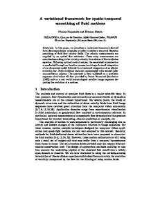
We consider a periodic domain of width 2𝜋. As an initial condition we use a repeated Weibull distribution, given by (9), with shape parameter 𝛼 = 2.5 and scale parameter 𝛽 = 2.5. The initial condition is propagated until 𝑡 = 4.5. 𝛼 𝛼 𝑢(𝑥) = 𝛼 𝑥𝛼−1 𝑒−(𝑥0 ∕𝛽) where 𝑥0 = 𝑥 mod 2𝜋 (9) 0 𝛽 For the diffusion equation we use Fourier analysis to obtain the solution at different time instants. Figure 1 a illustrates the evolution of the solution for a viscosity coefficient 𝜈 = 0.3. Figure 1 b plots energy spectra, according to (7), that correspond to the plotted solutions at different time instants. We observe that both the solutions and the associated energy spectra show a rapid damping of high frequency modes, emphasizing coarse-scale solution components. For the nonlinear transport equation we use the method of characteristics to advance the solution in time. Figure 2 a illustrates the evolution of the solution in time for the given initial condition. We observe that a shock wave is formed at the final time instant 𝑡 = 4.5. Figure 2 b plots energy spectra that correspond to the displayed solution fields at different times. We observe that in contrast to the diffusion equation, the nonlinear transport equation transfers energy towards the higher frequencies. The sharp gradient at the shock front requires a wide distribution of energy components in the frequency domain, emphasizing fine-scale solution components.

4

10 -3

u

Spectral energy E(k)

Initial condition

0.40 0.30 0.20 0.10

0

1

2

3

4

5

x

Initial

10 -9 10 -15

n

10 -21 10 -27 10 -33 0 10

6

condit io

(a) Spatial solutions.

10 1

10 2 Wave number k

(b) Energy spectra.

FIGURE 1 Solution of the diffusion equation at different time instants.

Spectral energy E(k)

u

10 -2

Initial condition

0.40 0.30 0.20 0.10

0

1

2

3

4

5

x

6

(a) Spatial solutions.

10 -4 10 -6 10

-8

Ini

tia l

con

dit ion

10 -10 10 -12 10 -14 0 10

10 1

10 2 Wave number k

(b) Energy spectra.

FIGURE 2 Solution of the nonlinear transport equation at different time instants.

2.3

Balance of energy spectra and Burgers turbulence

When the diffusion equation (3) and the transport equation (4) are combined to form the Burgers equation (1), the solution must represent a balance between the two conflicting energy evolutions. We illustrate the balance in the energy spectrum evolution with a numerical example described in 38 . We consider (1) on a periodic domain of width 2𝜋 with a viscosity coefficient 𝜈 = 2𝜋∕1000, a constant initial condition 𝑢(𝑡0 ) = 1, and a source function 𝑔(𝑥, 𝑡) = 0.1 sin(𝑥−𝑡) that is periodic in space and time. This problem was investigated in 38 . We discretize the domain with 8,192 linear finite elements in space and use the fifth-order accurate explicit Dormand-Prince Runge-Kutta method in time with a time-step size of Δ𝑡 = 3.2 ⋅ 10−5 . The spatial mesh resolution is thereby equal to that of the direct numerical simulation (DNS) described in 38 , while we use a smaller time step and a time integration method of higher order. Figures 3 a and 3 b plot solutions and corresponding energy spectra at different time instants. We observe that the periodic forcing creates a wave that travels to the right through the periodic domain. From 𝑡 = 6𝜋 onward, the shape of the wave that is translated through the periodic domain remains practically unchanged, so that the corresponding energy spectrum is steady. The steady energy spectrum shown in Figure 3 b illustrates the characteristic multiscale solution behavior of the Burgers equation. The nonlinear hyperbolic nature of the equation results in a solution that approaches a shock wave. In the frequency response, this corresponds to energy being transferred to the high frequency modes. At the high frequency range, the energy is dissipated by the viscous term of the equation. We note that the noisy behavior past 𝑘 = 103 is the result of the limited machine accuracy, where 𝐸(𝑘) ≈ 10−32 roughly corresponds to the square of the double-precision machine epsilon. As we use a sufficiently fine discretization in space and time, all scales of the Burgers solution can be resolved with sufficient accuracy. In practical applications, however, such a DNS discretization is prohibitively expensive, so that coarser discretizations must be used that can only represent the coarse-scale behavior of the PDE. As illustrated in Figure 3 b, the coarse-scale finite element solution (denoted by 𝑢) ̄ covers only the low frequency modes. In this situation, a subgrid-scale model, for example VMS

5

10 -2

1.8 Spectral energy E(k)

u 1.4 Initial condition

1.0 0.6 0.2

10 -8 10 -14 10 -20 10 -26 10 -32 10 -38

0

1

2

3

4

5

x

(a) Spatial solutions.

6

10 0

10 1

10 2 10 3 Wave number k

(b) Energy spectra.

FIGURE 3 DNS solution of the Burgers problem at different time instants. based, that reproduces the effect of the scale interaction with fine-scale solution components (denoted by 𝑢′ ) is essential for an accurate coarse-scale solution. Without a suitable subgrid-scale model, the coarse-scale solution will tend to overemphasize certain energy components, since they cannot be dissipated at the fine scales 38 . In the following sections, we will develop a residual-based fine-scale model that can be used in a discontinuous Galerkin variational multiscale formulation of the Burgers equation.

3 VARIATIONAL MULTISCALE FORMULATION IN A DISCONTINUOUS APPROXIMATION SPACE In this section, we extend the discontinuous Galerkin residual-based variational multiscale (DG-RVMS) method, introduced in 33 , to nonlinear hyperbolic problems with a viscous term. For a periodic domain Ω, this class of boundary value problems is defined as: { 𝑢𝑡 − 𝜈Δ𝑢 + ∇ ⋅ 𝑓 (𝑢) = 𝑔(𝑥, 𝑡) in Ω × (𝑡0 , 𝑇 ] (10) 𝑢 = 𝑢(𝑡0 ) on Ω × {𝑡0 } where 𝑓 (𝑢) is a (potentially nonlinear) flux function. We assume that the diffusion coefficient is sufficiently large to ensure that the true solution is at least 𝐶 1 -continuous in space and time. We emphasize that the class of problems described by (10) contains the Burgers model problem (1) as a special case.

3.1

Space-time variational multiscale formulation

Following the VMS procedure described in 5 , we divide the temporal domain into 𝑁 time slabs of domain (𝑡𝑛 , 𝑡𝑛+1 ), where 𝑛 = 0, ⋯ , 𝑁 −1. A separate initial boundary value problem can be posed for each time slab. The initial value within a time slab is the final value of the previous time slab. For discretizing the space-time domain, we consider the following function space: { } |  𝑛 (ℎ) = 𝑣 ∈ 𝐿2 (Ω × [𝑡𝑛 , 𝑡𝑛+1 ]) ∶ 𝑣| ∈  0 ∀ 𝑄 ∈ 𝑄 , 𝑣 = ℎ on Ω × {𝑡𝑛 } (11) |𝑄 where 𝑄 is a space-time element in the set of space-time elements 𝑄 = {𝑄} that spans the time slab. Figure 4 illustrates the space-time domain and its discretization for the case of a one-dimensional spatial domain. Each space-time element is constructed as a spatial element 𝐾 advanced in time: 𝑄 = 𝐾 × (𝑡𝑛 , 𝑡𝑛+1 ). For completeness, we also define a computational mesh  = {𝐾} which is the set of spatial elements. We emphasize that (11) allows trial and test functions that are discontinuous from element to element. We derive the weak formulation of problem (10) on each time slab by the method of weighted residuals that we individually apply to each space-time element. This ensures that the derivatives remain well-defined within the respective element domain. Additionally, we impose transmission conditions that act on the element interfaces to couple the elements and to ensure the

6

(a) Space-time domain.

(b) Discretization of the space-time domain.

FIGURE 4 Definition of the domain and discretization.

uniqueness of the solution. Making use of the definitions summarized in Table 1 , the weak formulation reads as follows: ( ) Find 𝑢 ∈  𝑛 𝑢(𝑡𝑛 ) s.t.: ⎧ ∑ (𝑤, 𝑢 − 𝜈Δ𝑢 + ∇ ⋅ 𝑓 (𝑢)) = ∑ (𝑤, 𝑔 ) ∀ 𝑤 ∈  𝑛 (0) 𝑡 𝑄 𝑄 ⎪𝑄∈ 𝑄∈ 𝑄 (12) ⎪ 𝑄 ⎨ [[𝑢]] = 0 on 𝜕𝑄 ∀ 𝑄 ∈ 𝑄 ⎪ ⎪ [[∇𝑢]] = 0 on 𝜕𝑄 ∀ 𝑄 ∈ 𝑄 ⎩ In the next step, we introduce the split of the true solution 𝑢 into a coarse-scale solution 𝑢̄ and a complementary fine-scale solution 𝑢′ . To define this split, we make use of the following definitions: |  𝑛 (𝑔) = {𝑣 ∈ 𝐿2 (Ω×[𝑡𝑛 , 𝑡𝑛+1 ]) ∶ 𝑣| ∈ 𝑃 𝑝 (𝑄) ∀ 𝑄 ∈ 𝑄 , 𝑣 = 𝑔 at 𝑡 = 𝑡𝑛 } (13) |𝐾 𝑛 (14) 𝑢̄ ≡ 𝑢 ∈  (⋅) 𝑢′ ≡ 𝑢 − 𝑢̄ ⇒ 𝑢 = 𝑢̄ + 𝑢′ ′

(15) ′

′𝑛

𝑢 = (𝑢 − 𝑢) ̄ = 𝑢 − (𝑢) = 0 ⇒ 𝑢 ∈ ker() ≡  (⋅)

(16)

The coarse-scale solution is the component of 𝑢 that can be precisely represented in the discontinuous computational approximation space  𝑛 , defined in (13). A projector  ∶  𝑛 →  𝑛 is required to obtain 𝑢̄ as a projection of 𝑢 onto  𝑛 , which is defined in (14). In (15), we define the fine-scale solution 𝑢′ as the difference between the true solution 𝑢 and the coarse-scale solution 𝑢. ̄ When the projector  is a linear, idempotent, surjective mapping, then the fine-scale solution is a member of the fine-scale space  ′𝑛 , defined in (16). By construction of the fine-scale function space  ′𝑛 , the coarse-scale and fine-scale function spaces form a direct sum decomposition of the space  𝑛 :  𝑛 =  𝑛 ⊕  ′𝑛

(17)

By definition of the direct sum decomposition (17), any possible true solution 𝑢 ∈  𝑛 maps uniquely to a coarse-scale solution 𝑢̄ ∈  𝑛 and a fine-scale solution 𝑢′ ∈  ′𝑛 . This ensures the well-posedness of the VMS formulation. By substituting the split (15) into the weak formulation (12), we obtain the following variational multiscale formulation: ( 𝑛) ( ) Find 𝑢, ̄ 𝑢′ ∈  𝑛 𝑢(𝑡 ̄ ) ×  ′𝑛 𝑢′ (𝑡𝑛 ) s.t.: ) ( ) ( ) ( ) ⎧( ′ ′ ′ ∀ 𝑤̄ ∈  𝑛 (0) ⎪ 𝑤̄ , 𝑢̄ 𝑡 + 𝑢𝑡 Ω𝑄 − 𝜈 𝑤̄ , Δ𝑢̄ + Δ𝑢 Ω𝑄 + 𝑤̄ , ∇ ⋅ 𝑓 (𝑢̄ + 𝑢 ) Ω𝑄 = 𝑤̄ , 𝑔 Ω𝑄 ⎪( ) ( ) ( ) ( ) (18) ∀ 𝑤′ ∈  𝑛 (0) ⎪ 𝑤′ , 𝑢̄ 𝑡 + 𝑢′𝑡 Ω − 𝜈 𝑤′ , Δ𝑢̄ + Δ𝑢′ Ω + 𝑤′ , ∇ ⋅ 𝑓 (𝑢̄ + 𝑢′ ) Ω = 𝑤′ , 𝑔 Ω 𝑄 𝑄 𝑄 𝑄 ⎨ ⎪ [[𝑢]] ̄ = −[[𝑢′ ]] on 𝜕𝑄 ∀ 𝑄 ∈ 𝑄 ⎪ ⎪ [[∇𝑢]] ̄ = −[[∇𝑢′ ]] on 𝜕𝑄 ∀ 𝑄 ∈ 𝑄 ⎩

7

[[𝑤]]

Jump operator

{ 𝑤}} ( ) 𝑤, 𝑢 𝐾 ⟨ ⟩ 𝑤 ⋅ 𝑛, 𝑢 𝜕𝐾

Average operator Volume 𝐿2 -inner product Surface 𝐿2 -inner product

= 𝑤+ ⋅ 𝑛+ + 𝑤− ⋅ 𝑛− ( ) = 21 𝑤+ + 𝑤− =∫ 𝑤⋅𝑢 𝐾

= ∫ 𝑤 ⋅ 𝑛𝑢 𝜕𝐾

Space domain

Ω

(Periodic)

Element space domain

𝐾

(With boundary 𝜕𝐾)

Space-time element

𝑄

Numerical space domain

Ω𝐾

Numerical space-time domain

Ω𝑄

Element interfaces

Γ

= 𝐾 × (𝑡𝑛 , 𝑡𝑛+1 ) (With boundary 𝜕𝐾) ⋃ ( ) ) ∑ ( 𝐾 s.t. 𝑤, 𝑢 Ω = 𝑤, 𝑢 𝐾 = 𝐾 𝐾∈ 𝐾∈ ⋃ ( ) ) ∑ ( = 𝑄 s.t. 𝑤, 𝑢 Ω = 𝑤, 𝑢 𝑄 𝑄 𝑄∈𝑄 ⋃ ⟨ ⟩ 𝑄∈𝑄 ∑ ⟨ ⟩ = 𝜕𝐾 s.t. 1, [[𝑢]] Γ = 1, 𝑢 ⋅ 𝑛 𝜕𝐾 𝐾∈

𝐾∈

TABLE 1 Collection of domain definitions.

In the next step, we will transfer the coarse-scale weak formulation (18) into a discrete discontinuous Galerkin format. To this end, we first perform element-wise integration by parts on the different terms to find the following weak formulation: ( 𝑛) Find 𝑢̄ ∈  𝑛 𝑢(𝑡 ̄ ) s.t.: ( ) ( ) ̄ 𝑢′ ) 𝑤̄ , 𝑢̄ 𝑡 Ω − 𝑤̄ 𝑡 , 𝑢′ Ω + 𝑙(𝑤, 𝑄 𝑄 ∑⟨ ( ) ⟩ ( ) (19) ̄ ∇𝑢̄ Ω − ̄ ∇𝑢̄ ⋅ 𝑛 𝜕𝐾×(𝑡𝑛 ,𝑡𝑛+1 ) − 𝜈Δ𝑤, ̄ 𝑢′ Ω + 𝑚(𝑤, ̄ 𝑢′ ) + 𝜈∇𝑤, 𝜈 𝑤, 𝑄

(

𝑄

𝐾∈

− ∇ ⋅ 𝑤̄ , 𝑓 (𝑢̄ + 𝑢′ )

)

(

Ω𝑄

̄ 𝑢, + ℎ(𝑤, ̄ 𝑢′ ) = 𝑤̄ , 𝑔

) Ω𝑄

∀ 𝑤̄ ∈  𝑛 (0)

The functionals 𝑙, 𝑚 and ℎ contain integrals at the element interfaces, involving the fine-scale solution. They originate from integration by parts on the different terms in the PDE. Specifically, 𝑙 involves fine-scale initial conditions, integrated over the element interfaces Ω𝐾 × {𝑡𝑛 , 𝑡𝑛+1 }, 𝑚 includes those terms that are obtained from the diffusion term integrated over the element interfaces Γ × (𝑡𝑛 , 𝑡𝑛+1 ), and ℎ includes the (nonlinear) integrals obtained from the hyperbolic term on the same interfaces. At this point, it is worthwhile to note that the current formulation includes two types of fine-scale terms that represent the complete scale interaction between the fine-scale and coarse-scale solutions. They can be classified into fine-scale volumetric terms that have already been examined in classical continuous VMS formulations, and fine-scale interface terms that are new. When we substitute the fine-scale contributions corresponding to the projector  from (16) into (19), we obtain the coarse-scale solution 𝑢̄ corresponding to (14). In practice, however, the exact form of these fine-scale terms is unknown. In the following, we will derive implicit relations for these fine-scale terms, which we can substitute into (19) to obtain a closed form of the variational coarse-scale problem.

3.2

General form of the fine-scale interface model

To remove fine-scale dependencies that appear in the functionals 𝑙, 𝑚 and ℎ in (19), we first leverage the following (exact) identities, which do not involve any approximation. The fine-scale solution on either side of an element boundary is written 𝑢′+ or 𝑢′− . By definition of the jump and average operators (see Table 1 ), the following identities hold: 1 𝑢′± 𝑛± = { 𝑢′ } 𝑛± + [[𝑢′ ]] 2 (20) ′± ± ± 1 ′ ∇𝑢 ⋅ 𝑛 = { ∇𝑢 } ⋅ 𝑛 + [[∇𝑢′ ]] 2

8

According to the transmission conditions in (18), the jump of the fine-scale solution is equal and opposite to the jump of the coarse-scale solution, thereby: 1 ̄ 𝑢′± 𝑛± = { 𝑢′ } 𝑛± − [[𝑢]] 2 (21) 1 ̄ ∇𝑢′± ⋅ 𝑛± = { ∇𝑢′ } ⋅ 𝑛± − [[∇𝑢]] 2 To eliminate all the fine-scale dependencies in 𝑙, 𝑚 and ℎ, we write the remaining fine-scale terms as functions of coarse-scale interface terms: 1 𝑢′± 𝑛± = Φ 𝑛± − [[𝑢]] ̄ 2 (22) 1 ∇𝑢′± ⋅ 𝑛± = Θ ⋅ 𝑛± − [[∇𝑢]] ̄ 2 where we introduce fine-scale interface models of the form { 𝑢′ } = Φ({{𝑢} ̄ }, [[𝑢]], ̄ { ∇𝑢} ̄ }, [[∇𝑢]], ̄ ⋯) (23) ′ ̄ }, [[𝑢]], ̄ { ∇𝑢} ̄ }, [[∇𝑢]], ̄ ⋯) { ∇𝑢 } = Θ({{𝑢} By substituting (22) into the functionals 𝑙, 𝑘 and ℎ in (19), we obtain a global formulation where all elements are coupled. The choice of the fine-scale interface model and the associated assumptions should directly reflect the physics of the fine-scale behavior of the specific PDE at hand. In the next section, we will illustrate this for the example of the Burgers equation. Together with the fine-scale volumetric model, the choice of the fine-scale interface model determines the projector (14) that defines the split (15) into a coarse-scale solution and a fine-scale solution.

3.3

General form of the fine-scale volumetric model

Classical VMS formulations that treat the fine-scale volumetric term with a residual-based model assume that the fine-scale solution vanishes on element interfaces 2,5 . In a DG setting, the fine-scale solution at element interfaces is generally non-zero, which follows directly from (21). When the coarse-scale DG solution exhibits large jumps across element interfaces, the finescale solution must have large values as well, therefore having a significant impact on the fine-scale volumetric term in (19). To accommodate the presence of nonhomogeneous fine-scale solution values at element boundaries, we propose the following modifications to the classical residual-based volumetric fine-scale model. We start by considering the fine-scale weak formulation in (18), where we may treat each space-time element separately, since all functions are discontinuous from element to element. On a space-time element 𝑄, we rewrite the fine-scale weak formulation in such a way that each term on the left-hand side contains fine-scale components. Assuming that the fine-scale solution 𝑢′ typically represents a small perturbation with respect to the coarse-scale solution 𝑢, ̄ we expand the flux function 𝑓 into a first-order Taylor approximation that is linear with respect to 𝑢′ : 𝑓 (𝑢̄ + 𝑢′ ) = 𝑓 (𝑢) ̄ +

d𝑓 (𝑢)𝑢 ̄ ′ d𝑢

+ (𝑢′2 )

We substitute this approximation into the fine-scale weak formulation and obtain: ( ) Find 𝑢̃ ′ ∈  ′𝑛 𝑢′ (𝑡𝑛 ) s.t.: ) ( ) ( ′ ′) ( ) ( (𝑢) ̄ 𝑄 + 𝑤′ , d𝑓 (𝑢) ̄ ∇ ⋅ 𝑢̃ ′ 𝑄 𝑤 , 𝑢̃ 𝑡 𝑄 − 𝜈 𝑤′ , Δ𝑢̃ ′ 𝑄 + 𝑤′ , 𝑢̃ ′ ∇ ⋅ d𝑓 d𝑢 d𝑢 ( ) ( ) = 𝑤′ , 𝑔 − 𝑢̄ 𝑡 + 𝜈Δ𝑢̄ − ∇ ⋅ 𝑓 (𝑢) ̄ 𝑄 = 𝑤′ , 𝑢̄ 𝑄

(24)

(25) ′

𝑛

∀ 𝑤 ∈  (0)

where 𝑢̃ ′ is the approximate fine-scale solution and the source term 𝑢̄ on the right-hand side is the residual of the coarse-scale solution. We observe that the left-hand side in (25) is linear with respect to 𝑢̃ ′ , such that it can be rewritten as: ( ) Find 𝑢̃ ′ ∈  ′𝑛 𝑢′ (𝑡𝑛 ) s.t.: ( ′ ) ( ) (26) 𝑤 , 𝑢̄ 𝑢̃ ′ 𝑄 = 𝑤′ , 𝑢̄ 𝑄 ∀ 𝑤′ ∈  𝑛 (0) where the linear differential operator 𝑢̄ corresponds to the differential operator on the left-hand side of (25), assuming 𝑢̄ is known. Next, we use Green’s identities to rewrite the left-hand side term in (26) as: ( ) Find 𝑢̃ ′ ∈  ′𝑛 𝑢′ (𝑡𝑛 ) s.t.: ( ∗ ′ ′) ( ) (27) 𝑢̄ 𝑤 , 𝑢̃ 𝑄 + 𝑘(𝑤′ , 𝑢̃ ′ ; 𝜕𝑄) = 𝑤′ , 𝑢̄ 𝑄 ∀ 𝑤′ ∈  𝑛 (0)

9

where 𝑘( ⋅ , ⋅ ; 𝜕𝑄) is the collection of element interface terms that act on 𝜕𝑄 and appear as a result of integration by parts, and ∗𝑢̄ is the adjoint of 𝑢̄ . The definition of the Green’s function for the linearized PDE at hand is: ⎧ 𝐺(𝑥, 𝑦) ∈  𝑛 (0) ⎪ ∗ (28) ⎨ 𝑢̄ 𝐺(𝑥, 𝑦) = 𝛿𝑥 for 𝑦 ∈ 𝑄 ⎪ for 𝑦 ∈ 𝜕𝑄 ⎩ 𝐺(𝑥, 𝑦) = 0 We choose the Green’s function defined in (28) as the test function 𝑤′ . Substituting 𝐺(𝑥, 𝑦) in place of 𝑤′ in (27), we obtain: ∫

∗𝐺(𝑥, 𝑦) 𝑢̃ ′ d𝑦 =

∫

𝛿𝑥 𝑢̃ ′ d𝑦 = 𝑢̃ ′ = −𝑘(𝐺(𝑥, 𝑦), 𝑢̃ ′ ; 𝜕𝑄) +

𝐺(𝑥, 𝑦) 𝑢̄ d𝑦

(29)

𝑄

𝑄

𝑄

∫

where the parameter of integration and differentiation is 𝑦. Equation (29) is driven by the coarse-scale residual via its last term. It also depends on the fine-scale boundary conditions via the functional 𝑘. To close the formulation, the fine-scale boundary values 𝑢̃ ′ must be written in terms of the coarse-scale solution, for which the identities in (21) can be used. Since the fine-scale solution 𝑢̃ ′ occurs in the volumetric term in a weighted sense, we can implement all Green’s functions as averaged quantities: ) ( ∗ ) ( ) ( ̄ 𝑢′ 𝑄 ≈ ∗𝑤, ̄ −𝑘(𝐺(𝑥, 𝑦), 𝑢̃ ′ ; 𝜕𝑄) 𝑄 + 𝐺(𝑥, 𝑦) 𝑢̄ d𝑦 𝑄 (30)  𝑤, ∫ ∑ ( ̄ ≈ − ∗𝑤, 𝛾𝐹 𝐹 ∈𝜕𝑄

𝑄

) ( ) 1 ̄ 𝜏𝑢̄ 𝑄 ( − [[𝑢]] ̄ ⋅ 𝑛) 𝑄 + ∗𝑤, ∫ Φ 2

(31)

𝐹

where 𝐹 denotes the faces (3D), edges (2D) or nodes (1D) of the element 𝐾, and 𝜏 and 𝛾𝐹 are averaged Green’s function quantities. Relation (31) is inspired by the steady advection-diffusion equation with constant coefficients in one dimension, where it is an identity when discretized with linear basis functions. In (31), the averaged Green’s function quantities are defined as: 𝜏=

1 𝐺(𝑥, 𝑦) d𝑦 d𝑥 |𝑄| ∫ ∫ 𝑄

𝑄

𝛾𝐹 =

1 (𝑥, 𝑦) d𝑦 d𝑥 |𝑄| ∫ ∫ 𝑄

(32)

𝐹

where  is a function derived from the Green’s function, which depends on the definition of 𝑘, as we will show for the example of the Burgers equation in the next section.

4

A DG-RVMS FORMULATION FOR THE BURGERS EQUATION

In this section, we apply the general DG-RVMS framework described above to a one-dimensional viscous Burgers equation, which can be obtained from (10) with the following flux function: 1 𝑓 (𝑢) = 𝑢2 (33) 2 For the discretization in time, finite difference schemes are commonly preferred over space-time finite element methods in most practical applications. We therefore use a finite element formulation in space only, for which the weak formulation is written as: Find 𝑢 ∈  s.t.: ( ) ⎧( 1 2 ) ∀ 𝑤 ∈ (0) ⎪ 𝑤, 𝑢𝑡 − 𝜈𝑢𝑥𝑥 + 2 (𝑢 )𝑥 Ω𝐾 = 𝑤, 𝑔 Ω𝐾 (34) ⎪ on Γ ⎨ [[𝑢]] = 0 ⎪ on Γ ⎪ [[∇𝑢]] = 0 ⎩ where  is the purely spatial function space equivalence of (11). For the development of the fine-scale volumetric model, we still make use of the space-time formulation described in the previous section. In doing so, we interpret a finite difference step in time from 𝑡𝑛 to 𝑡𝑛+1 as one time-slab.

10

4.1

The coarse-scale DG-RVMS system

Using the multiscale split (15) and integration by parts as described in Section 3, we obtain the following coarse-scale weak formulation, analogous to (19): Find 𝑢̄ ∈  s.t.: ∑ [⟨ ( ) ( ) ( ) ⟩ ⟨ ⟩ ⟨ ⟩ ] ̄ 𝑢̄ 𝑡 +𝑢′𝑡 Ω + 𝑤̄ 𝑥 , 𝜈 𝑢̄ 𝑥 Ω − 𝑤̄ 𝑥𝑥 , 𝜈𝑢′ Ω + 𝑤, 𝑤̄ 𝑛, 𝜈 𝑢̄ 𝑥 𝜕𝐾 − 𝑤̄ 𝑛, 𝜈𝑢′𝑥 𝜕𝐾 − 𝑤̄ 𝑥 , 𝜈𝑢′ 𝑛 𝜕𝐾 𝐾

𝐾

𝐾

𝐾∈ ∑ 1⟨ ) ( ) ) ( )2 ⟩ 1( 1( − 𝑤̄ 𝑥 , 𝑢̄ 2 Ω − 𝑤̄ 𝑥 , 𝑢̄ 𝑢′ Ω − 𝑤̄ 𝑥 , 𝑢′ 2 Ω + 𝑤̄ 𝑛, 𝑢̄ + 𝑢′ 𝜕𝐾 𝐾 𝐾 𝐾 2 2 2 𝐾∈ ( ) ̄ 𝑓 Ω = 𝑤, ∀ 𝑤̄ ∈ 

(35)

𝐾

First, we focus on the interface terms that are related to the diffusion term. We substitute the identity (21) and obtain: ∑ [⟨ ⟩ ⟨ ⟩ ⟨ ⟩ ] 𝑤̄ 𝑛, 𝜈 𝑢̄ 𝑥 𝜕𝐾 − 𝑤̄ 𝑛, 𝜈𝑢′𝑥 𝜕𝐾 − 𝑤̄ 𝑥 , 𝜈𝑢′ 𝑛 𝜕𝐾 = 𝐾∈

⟩ ⟨ ⟩ ⟨1 ⟩ ] ⟨ ⟩ ⟨1 ′ ′ ̄ ̄ ̄ ̄ 𝑤, 𝜈[[ 𝑢 ̄ ]] + 𝑤 𝑛, 𝜈{ { 𝑢 } − 𝑤 , 𝜈[[ 𝑢]] ̄ = − 𝑤 𝑛, 𝜈{ { 𝑢 } + 𝑥 𝑥 𝑥 𝜕𝐾 𝜕𝐾 𝜕𝐾 𝜕𝐾 𝜕𝐾 2 2 𝑥 𝑘∈ ∑ [⟨ ⟩ ] ⟨ ⟩ ⟨ ⟩ ⟨ ⟩ ⟨ ⟩ ̄ 𝜈{{𝑢′𝑥 } Γ + { 𝑤} ̄ }, 𝜈[[𝑢̄ 𝑥 ]] Γ + [[𝑤]] ̄ 𝑥 , 𝜈{{𝑢′ } Γ − { 𝑤̄ 𝑥 } , 𝜈[[𝑢]] 𝑤̄ 𝑛, 𝜈 𝑢̄ 𝑥 𝜕𝐾 − [[𝑤]], ̄ Γ ∑ [⟨

𝑘∈

𝑤̄ 𝑛, 𝜈 𝑢̄ 𝑥

⟩

(36)

⟨ ⟩ ⟨ ⟩ ⟨ ⟩ ⟨ ⟩ ̄ 𝜈{{𝑢′𝑥 } Γ − [[𝑤]], ̄ 𝜈{{𝑢̄ 𝑥 } Γ + [[𝑤]] ̄ 𝑥 , 𝜈{{𝑢′ } Γ − { 𝑤̄ 𝑥 } , 𝜈[[𝑢]] = − [[𝑤]], ̄ Γ

where, from the third to the fourth line, we use the following identity: ⟨ ⟩ ⟨ ⟩ ⟨ ⟩ ̄ }, [[𝑢̄ 𝑥 ]] 𝜕𝐾 − 𝑤, ̄ 𝑢̄ 𝑥 𝑛 𝜕𝐾 + − 𝑤, ̄ 𝑢̄ 𝑥 𝑛 𝜕𝐾 − { 𝑤} ( ) 1 + = (𝑤̄ + 𝑤̄ − )(𝑢̄ +𝑥 𝑛+ + 𝑢̄ −𝑥 𝑛− ) − (𝑤̄ 𝑢̄ 𝑥 𝑛)+ − (𝑤̄ 𝑢̄ 𝑥 𝑛)− ∫ 2 𝐾 ( ) 1 − 𝑤̄ + 𝑛+ 𝑢̄ +𝑥 − 𝑤̄ + 𝑛+ 𝑢̄ −𝑥 − 𝑤̄ − 𝑛− 𝑢̄ +𝑥 − 𝑤̄ − 𝑛− ∇𝑢̄ − = ∫ 2 𝐾 ⟨ ⟩ 1 + + ̄ { 𝑢̄ 𝑥 } 𝜕𝐾 =− (𝑤̄ 𝑛 + 𝑤̄ − 𝑛− )(𝑢̄ −𝑥 + 𝑢̄ +𝑥 ) = − [[𝑤]], ∫ 2

(37)

𝐾

Next, we focus on the interface terms that are related to the nonlinear advective term. Due to the continuity of the true solution 𝑢, we can infer that 𝑢̄ + 𝑢′ = 𝑢 is single-valued on element interfaces. We can therefore write: ∑ 1⟨ ( )2 ⟩ ⟩ ⟩ ⟩ 1⟨ 1⟨ 1⟨ ̄ 𝑢2 Γ = ̄ { 𝑢}}2 Γ = ̄ { 𝑢̄ + 𝑢′ } 2 Γ 𝑤̄ 𝑛, 𝑢̄ + 𝑢′ = [[𝑤]], [[𝑤]], [[𝑤]], 𝜕𝐾 2 2 2 2 𝐾∈ (38) ⟨ ( ) ⟩ ⟨ ⟩ 2 1 1 2 ′ ′ 2 ̄ ̄ = [[𝑤]], { 𝑢} ̄ } + { 𝑢′ } = [[ 𝑤]], { 𝑢} ̄ } + 2{ { 𝑢} ̄ } { 𝑢 } + { 𝑢 } Γ Γ 2 2 By substituting the manipulated interface terms of (36) and (38) into (35), we obtain the following coarse-scale weak formulation: Find 𝑢̄ ∈  s.t.:

(

) ( ) ( ) ̄ 𝑢̄ 𝑡 + 𝑢′𝑡 Ω + 𝑤̄ 𝑥 , 𝜈 𝑢̄ 𝑥 Ω − 𝑤̄ 𝑥𝑥 , 𝜈𝑢′ Ω 𝑤, 𝐾 𝐾 𝐾 ⟨ ⟩ ⟨ ⟩ ⟨ ⟩ ⟨ ⟩ ̄ 𝜈 { 𝑢̄ 𝑥 } Γ − { 𝑤̄ 𝑥 } , 𝜈 [[𝑢]] ̄ 𝜈 { 𝑢′𝑥 } Γ + [[𝑤̄ 𝑥 ]], 𝜈 { 𝑢′ } Γ − [[𝑤]], ̄ Γ − [[𝑤]], ) ( ) ) 1( 1( − 𝑤̄ 𝑥 , 𝑢̄ 2 Ω − 𝑤̄ 𝑥 , 𝑢̄ 𝑢′ Ω − 𝑤̄ 𝑥 , 𝑢′ 2 Ω 𝐾 𝐾 𝐾 2 2 1⟨ 2⟩ 2 ′ ′ ̄ { 𝑢} + [[𝑤]], ̄ } + 2{{𝑢} ̄ }{ 𝑢 } + { 𝑢 } Γ 2 ( ) ̄ 𝑓 Ω = 𝑤, ∀ 𝑤̄ ∈ 

(39)

𝐾

We emphasize again that no approximations or simplifications have been introduced until this point. This means that the coarsescale formulation (39) captures the complete multiscale nature of the PDE.

11

4.2

A fine-scale interface model for the Burgers equation

To eliminate the fine-scale dependencies in the interface terms of (39), we propose the following fine-scale interface model, in reference to (23): ⎧ = { 𝑢′ } = 0 on Γ ⎪Φ (40) ⎨ 1 −1 ̄ }|) [[𝑢]] ̄ on Γ ⎪ Θ = { 𝑢′𝑥 } = −(𝜂ℎ + |{{𝑢} 2𝜈 ⎩ where 𝜂 is a model parameter, ℎ is the mesh size, and the viscous-like term 𝜈 is assumed constant. Substituting the first line of (40) in (39) removes the fine-scale interface term that originates from the Laplace operator and all fine-scale interface terms that originate from the nonlinear advection term. We then substitute the second line of (40) into the remaining fine-scale interface term. We combine the result with the coarse-scale nonlinear advection term as follows: ⟨ ⟩ ⟩ ⟨ ⟩ ( )⟩ 1⟨ 1⟨ 1 (41) ̄ 𝜈 { 𝑢′𝑥 } Γ + ̄ { 𝑢} ̄ 𝜈𝜂ℎ−1 [[𝑢]] ̄ { 𝑢} − [[𝑤]], [[𝑤]], ̄ }2 Γ = [[𝑤]], ̄ Γ+ [[𝑤]], ̄ } sign({{𝑢} ̄ }) [[𝑢]] ̄ + { 𝑢} ̄} Γ 2 2 2 The last term in (41) can be manipulated as follows: ⟩ ( )⟩ 1⟨ 1⟨ 1 1 ̄ { 𝑢} ̄ { 𝑢} [[𝑤]], ̄ }(sign({{𝑢} ̄ })[[𝑢]] ̄ + { 𝑢} ̄ }) Γ = [[𝑤]], ̄ } sign({{𝑢} ̄ }) (𝑢̄ − − 𝑢̄ + ) + (𝑢̄ − + 𝑢̄ + ) Γ 2 2 2 2 ⟩ ⎧1⟨ ̄ { 𝑢} ̄ } 𝑢̄ − Γ if { 𝑢} ̄} > 0 ⎪ [[𝑤]], (42) = ⎨ 12 ⟨ ⟩ + ̄ { 𝑢} ̄ } 𝑢̄ Γ if { 𝑢} ̄} < 0 ⎪ 2 [[𝑤]], ⎩ ⟩ 1⟨ ̄ { 𝑢} = [[𝑤]], ̄ } 𝑢( ̄ lim 𝑥 − 𝜖{{𝑢} ̄ }) Γ 𝜖→0 2 where at each interface, 𝑢̄ − is evaluated on the element on the left and 𝑢̄ + is evaluated on the element on the right. The final coarse-scale variational formulation that we obtain with the fine-scale interface model (40) is: Find 𝑢̄ ∈  s.t.:

(

( ) ( ) + 𝑤̄ 𝑥 , 𝜈 𝑢̄ 𝑥 Ω − 𝑤̄ 𝑥𝑥 , 𝜈𝑢′ Ω 𝐾 𝐾 ⟨ ⟩ ⟨ ⟩ ⟨ ⟩ ̄ 𝜈 { 𝑢̄ 𝑥 } Γ − { 𝑤̄ 𝑥 } , 𝜈 [[𝑢]] ̄ 𝜂ℎ−1 𝜈 [[𝑢]] − [[𝑤]], ̄ Γ + [[𝑤]], ̄ Γ ) ( ) ) ⟩ 1( 1( 1⟨ ̄ { 𝑢} − 𝑤̄ 𝑥 , 𝑢̄ 2 Ω − 𝑤̄ 𝑥 , 𝑢̄ 𝑢′ Ω − 𝑤̄ 𝑥 , 𝑢′ 2 Ω + [[𝑤]], ̄ } 𝑢( ̄ lim 𝑥 − 𝜖{{𝑢} ̄ }) Γ 𝜖→0 𝐾 𝐾 𝐾 2 2 2 ( ) ̄ 𝑓 Ω = 𝑤, ∀ 𝑤̄ ∈  ̄ 𝑢̄ 𝑡 + 𝑢′𝑡 𝑤,

)

Ω𝐾

(43)

𝐾

Our DG-RVMS formulation originates completely from a variational multiscale point of view. It is interesting to note, however, that it features components that closely resemble classical DG formulations. For example, the fine-scale interface model can be interpreted as combining an interior penalty (IP) treatment of the diffusion term with an upwinding treatment of the advective term. For the upwind method, an advective velocity of magnitude 𝑢 = { 𝑢} ̄ } is used. Therefore, the DG-RVMS point of view offers a multiscale interpretation of classical formulations. In particular, we may conclude that when the fine-scale volume terms are treated appropriately, the use of an IP method combined with an upwind method implicitly enforces a projector that corresponds to the fine-scale interface model (40). We refer the interested reader to our earlier work 33 , where we studied the nature of this projector in more detail.

4.3

A fine-scale volumetric model for the Burgers equation

To eliminate the fine-scale dependencies in the volumetric terms of (39), we derive a volumetric fine-scale model based on the space-time fine-scale weak formulation described in Section 3.3. We note that we neglect the fine-scale time derivative in the first term of (43), which is common practice 5 . For the one-dimensional case, we develop a fine-scale volumetric model of the form: 1 1 | | 𝑢′ ≈ 𝜏𝑢̄ + 𝛾0 [[𝑢]] ̄ | − 𝛾1 [[𝑢]] ̄ | (44) | |𝑥𝑗+1 𝑥 2 2 𝑗 where the point 𝑥𝑗 corresponds to the left node of the current element in which 𝑢′ is to be modeled, and 𝑥𝑗+1 to the right node. We observe that relation (44) corresponds to (31), with the fine-scale interface model Φ from (40).

12

We obtain the definitions of 𝜏, 𝛾0 and 𝛾1 from the fine-scale problem. Following the residual-based strategy described in Section 3.3, the fine-scale problem can be written as: Find 𝑢̃ ′ ∈  ′ (0) s.t.: ( ′ ′ ) ( ) 𝑤 , 𝑢̃ 𝑡 − 𝜈 𝑢̃ ′𝑥𝑥 + 𝑢̄ 𝑥 𝑢̃ ′ + 𝑢̄ 𝑢̃ ′𝑥 𝑄 = 𝑤′ , 𝑢̄ 𝑄

∀ 𝑤′ ∈ (0)

(45)

Thereby, we may define the linearized fine-scale differential operator, its adjoint and the accompanying interface integrals as: d d2 d + 𝑢̄ 𝑥 + 𝑢̄ −𝜈 2  = d𝑡 d𝑥 d𝑥 d d2 d −𝜈 2 ∗ = − + 𝑢̄ 𝑥 − 𝑢̄ d𝑡 d𝑥 d𝑥 (46) ⟨ ⟩ ⟨ ′ ′⟩ ′ ′ ′ ′ 𝑘(𝑤 , 𝑢 ) = − 𝑤 , 𝑛𝑢 Υ𝑛 + 𝑤 , 𝑢 Υ𝑛+1 + ⟨ ′ ⟩ ⟨ ⟩ ⟨ ⟩ 𝑤 𝑛 , 𝑢𝑢 ̄ ′ 𝜒 − 𝑤′ 𝑛, 𝜈𝑢′𝑥 𝜒 + 𝑤′𝑥 , 𝜈 𝑛 𝑢′ 𝜒 where Υ refers to the temporal boundary of 𝜕𝑄, and 𝜒 to the spatial boundary. We construct the parameter 𝜏 associated to the Burgers equation by means of asymptotic scaling arguments. The behavior of the PDE depends on the set of parameters 𝜈, 𝑢̄ 𝑥 and 𝑢. ̄ Their values determine which differential operators dominate the collective 𝜏. We expect the following asymptotic behavior: 1 ≫ 𝜈, 𝑢̄ 𝑥 , 𝑢̄

⇒

𝜏 → 𝜏𝑡 =

𝑢̄ 𝑥 ≫ 1, 𝜈, 𝑢̄

⇒

𝜏 → 𝜏𝑅 =

𝑢̄ ≫ 1, 𝑢̄ 𝑥 , 𝜈

⇒

𝜏 → 𝜏𝐴 =

𝜈 ≫ 1, 𝑢, ̄ 𝑢̄ 𝑥

⇒

𝜏 → 𝜏𝐷 =

(𝑡𝑛+1 −𝑡𝑛 )2 2ℎ 𝑝−1 1 𝐶 𝑢̄ 𝑥 2

𝐶1𝑞−1

ℎ 𝐶 𝑝−1 2𝑢̄ 2 ℎ2 𝐶 𝑝−1 12𝜈 2

(47)

where 𝜏𝑡 corresponds to the Green’s function of a purely temporal differential operator d𝑡d . Similarly, 𝜏𝑅 , 𝜏𝐴 and 𝜏𝐷 correspond to the reactive, advective and diffusive components, respectively. Explicit expressions for these Green’s function quantities are derived in A. We add factors 𝐶1𝑘−1 and 𝐶2𝑝−1 to mitigate the averaging error introduced in (31) when using higher-order basis functions. Here, 𝑝 and 𝑞 denote the polynomial degree of the finite element discretization and the convergence rate of the finite difference time integration method. We note that the coefficients 𝐶1 and 𝐶2 should be smaller than 1 to enable convergence. In our numerical experiments, however, we found that larger values sometimes yield better results. The final 𝜏 is constructed from the single components in (47) as follows: 1 𝜏=√ (48) ( )2 ( )2 ( )2 ( )2 1 1 1 1 + 𝜏 + 𝜏 + 𝜏 𝜏 𝑡

𝑅

𝐴

𝐷

where we follow the asymptotic scaling argument that is commonly used to derive stabilization parameters in stabilized finite element methods 39 . The definition of 𝛾 can be based on the interface integrals in (46), where we replace the test function 𝑤′ by the Green’s function. Since the Green’s function is by definition zero on the element boundaries, only the last term remains. Comparing this term to the definition of 𝛾 in (32), we find: d (49) (𝑥, 𝑦) = 𝜈 𝐺(𝑥, 𝑦) d𝑦 Similar to the construction of 𝜏, a 𝛾 expression can be derived for each differential operator (temporal, reactive, advective and diffusive). As shown in A, for the present case, only the 𝛾 that corresponds to the diffusion operator is non-zero. In our numerical experiments, we will use: 1 𝐶 𝛾0 = 2𝜈 3 (50) 1 𝛾1 = − 𝐶3 2𝜈 We introduce another factor, 𝐶3 , for the same reason as above, i.e., to mitigate the averaging error.

13

5

NUMERICAL EXPERIMENTS

In this section, we will illustrate the potential of the DG-RVMS formulation and the associated fine-scale models to improve the accuracy of the finite element solution by incorporating subgrid-scale behavior of the one-dimensional Burgers model problem. To this end, we return to the Burgers benchmark that we introduced in Section 2.3 and whose solution and energy spectra are plotted in Figure 3 . We use the result of the DNS discretization presented in Section 2.3 as the reference solution. Our DGRVMS formulation is based on (43), with the volumetric fine-scale model derived in Section 4.3. We use the classical explicit fourth-order Runge-Kutta method (RK4) for time integration, where we interpret the time-step 𝑡𝑛 → 𝑡𝑛+1 as a time-slab in the volumetric fine-scale model. The RK4 algorithm produces a solution 𝑢̄ at 𝑡𝑛+1 based on the known solution at 𝑡𝑛 and a weighted average of intermediate time derivatives. The intermediate time derivatives are obtained from the coarse-scale formulation, where we use the solution 𝑢̄ of the previous intermediate computation for the explicit treatment of all coarse-scale terms. This includes the residual and interface jumps in the volumetric fine-scale model (44). The following numerical experiments use a time step size of Δ𝑡 = 𝜋∕(8 𝑝 𝑁), where 𝑝 is the polynomial order of the DG basis functions and 𝑁 the total number of elements. The RK4 method is fourth order accurate in total accumulated error, yet fifth order accurate in the local truncation error, and hence 𝑞 = 5 in (47).

Accuracy in solution fields

5.1

Figures 5 to 7 show the resulting solutions at times 𝑡 = 7.75𝜋 and 𝑡 = 8𝜋, obtained with four DG elements and higher-order basis functions of polynomial order 𝑝 = 2, 𝑝 = 3 and 𝑝 = 4, respectively. At time 𝑡 = 7.75𝜋, the wave front lies in the center of an element, and at time 𝑡 = 8𝜋, it lies in between two elements. We compute two solutions that include a residual based

2.0

2.0

DNS solution No vol. model CG-RVMS DG-RVMS

u 1.5

DNS solution No vol. model CG-RVMS DG-RVMS

u 1.5

1.0

1.0

0.5 0.5 0.0

0

1

2

3

4

5

x

6 0.0

0

1

2

3

4

5

0.5

(a) At 𝑡 = 7.75𝜋

x

6

(b) At 𝑡 = 8𝜋

FIGURE 5 Example solutions with and without proposed DG-RVMS model. Using 4 DG elements of 𝑝 = 2. 2.0

2.0

DNS solution No vol. model CG-RVMS DG-RVMS

u 1.5

1.5

1.0

1.0

0.5

0.5

0.0

0

1

2

3

(a) At 𝑡 = 7.75𝜋

4

5

x

DNS solution No vol. model CG-RVMS DG-RVMS

u

6

0.0

0

1

2

3

4

5

x

(b) At 𝑡 = 8𝜋

FIGURE 6 Example solutions with and without proposed DG-RVMS model. Using 4 DG elements of 𝑝 = 3.

6

14

2.0

2.0

DNS solution No vol. model CG-RVMS DG-RVMS

u 1.5

1.5

1.0

1.0

0.5

0.5

0.0

0

1

2

3

4

(a) At 𝑡 = 7.75𝜋

5

x

DNS solution No vol. model CG-RVMS DG-RVMS

u

6

0.0

0

1

2

3

4

5

x

6

(b) At 𝑡 = 8𝜋

FIGURE 7 Example solutions with and without proposed DG-RVMS model. Using 4 DG elements of 𝑝 = 4.

fine-scale model. These are the ‘DG-RVMS’ solution, which includes the newly introduced jump-terms in formulation (44), and the ‘CG-RVMS’ solution, which excludes those terms (i.e. 𝐶3 = 0). Both RVMS solutions were obtained with constants 𝐶1 = 3 and 𝐶2 = 0.7, while the DG-RVMS solution also uses 𝐶3 = 0.3. Each figure compares the RVMS solutions to the DNS reference solution and a solution that was obtained without any volumetric fine-scale model. We observe that with respect to the DNS reference, the RVMS formulation consistently improves the accuracy of the solution. The oscillations within the elements become smaller and the jumps from element to element decrease. We observe that the CG-RVMS solution is slightly less accurate than the DG-RVMS solution.

5.2

Convergence of kinetic energy

As shown in Figures 5 to 7 , the DG method that excludes a volumetric model is already performing very well by itself due to the simplicity of the model problem. Hence, the quality of the solution field itself is not the most appropriate indicator for the performance of the DG-RVMS method. In Section 2, we reviewed the scale interaction in the Burgers equation, which revolves around the transfer of energy between coarse-scale and fine-scale solution components. We can therefore expect that the error in the total kinetic energy, as defined in (8), is a much more adequate measure for the performance of the DG-RVMS method and its associated fine-scale models. In the following, we examine the convergence of the relative total kinetic energy of the solution at time 𝑡 = 8𝜋, when the DG discretization in space is uniformly refined. The relative energy is computed with respect to the energy of the DNS solution averaged over the time window 6𝜋 ≤ 𝑡 ≤ 8𝜋, where the wave form of the solution is steady. We perform three sets of experiments to assess the energy convergence of the DG-RVMS formulation, which we report in Figures 8 to 10 for DG meshes of polynomial order 𝑝 = 2, 𝑝 = 3 and 𝑝 = 4, respectively. In each figure, we plot the energy errors that were obtained with the DG-RVMS model, the CG-RVMS model (𝐶3 = 0) and without a volumetric fine-scale model. Each of the figures is complemented by a table that shows the coefficients that were used at different mesh resolutions. For the DG-RVMS case, the coefficients 𝐶1 and 𝐶2 were kept at a constant value of 0.7, while the coefficient 𝐶3 was optimized empirically. For the CG-RVMS case, the coefficient 𝐶2 was kept at 0.7 and the coefficient 𝐶1 was optimized empirically. We observe that the DG-RVMS method is able to decrease the relative energy error of the solution by almost one order of magnitude with respect to the DG method without a volumetric fine-scale model. The three figures confirm that the improvement in energy accuracy occurs consistently for the complete range of mesh sizes and for all polynomial orders examined. It is interesting to see that the CG-RVMS model does not improve the energy accuracy. This indicates that the fine-scale boundary values included in the fine-scale volumetric model as proposed in Section 3.3 play a pivotal role for the optimal performance of the DG-RVMS formulation.

15

10-2 No vol. model CG-RVMS DG-RVMS

Rel. error of Etot

10-3

10-4

10-5

10-6

10-7 1 10

Model 1

Model 2

Dofs

𝐶1&2

𝐶3

𝐶1

𝐶2

12

0.7

0.1

3.0

0.7

24

0.7

0.1

3.0

0.7

48

0.7

0.1

2.0

0.7

96

0.7

0.1

2.0

0.7

192

0.7

0.1

0.7

0.7

384

0.7

0.1

0.7

0.7

2

10 # degrees of freedom

FIGURE 8 Energy convergence with uniform mesh refinement at 𝑡 = 8𝜋 for basis functions of 𝑝 = 2. 10-1

Rel. error of Etot

10

No vol. model CG-RVMS DG-RVMS

-2

10-3 10-4 10

-5

10-6 10-7 1 10

Model 1

Model 2

Dofs

𝐶1&2

𝐶3

𝐶1

𝐶2

16

0.7

0.3

3.0

0.7

32

0.7

0.2

3.0

0.7

64

0.7

0.2

2.0

0.7

128

0.7

0.1

0.7

0.7

256

0.7

0.025

0.7

0.7

102 # degrees of freedom

FIGURE 9 Energy convergence with uniform mesh refinement at 𝑡 = 8𝜋 for basis functions of 𝑝 = 3. 10-1 No vol. model CG-RVMS DG-RVMS

Rel. error of Etot

10-2

Model 1

Model 2

Dofs

𝐶1&2

𝐶3

𝐶1

𝐶2

10

0.7

0.3

3.0

0.7

20

0.7

0.3

3.0

0.7

40

0.7

0.3

2.0

0.7

80

0.7

0.3

0.7

0.7

160

0.7

0.025

0.7

0.7

10-3

10-4

10-5

10

-6

101

102 # degrees of freedom

FIGURE 10 Energy convergence with uniform mesh refinement at 𝑡 = 8𝜋 for basis functions of 𝑝 = 4.

16

5.3

Accuracy of energy spectra

DNS solution No vol. model DG-RVMS

Spectral energy E(k)

10-1

10-2

10-3

100

Absolute error in spectral energy

As a final measure of accuracy, we plot the energy spectra for a set of solutions. As discussed in Section 2, we can obtain these spectra by means of a fast Fourier transform that transfers a solution field from its spatial representation to its frequency domain. We average the energy spectra over the time window 6𝜋 ≤ 𝑡 ≤ 8𝜋, where the wave form of the solution is steady. We perform this analysis for models that include, and exclude, the DG-RVMS fine-scale volumetric model. Figures 11 to 13 plot the energy spectra and the associated error for each wave number for three coarse meshes of polynomial degree 𝑝 = 2, 𝑝 = 3, and 𝑝 = 4, respectively. The error in the spectra is computed with respect to the spectrum of the DNS solution averaged over the time window 6𝜋 ≤ 𝑡 ≤ 8𝜋. We observe that the DG-RVMS method consistently performs better than the variant that excludes the volumetric fine-scale model. This improvement occurs primarily in the low-frequency range, where the spectral energy is significantly closer to the DNS reference spectrum. This observation confirms that the DG-RVMS formulation reduces the spurious energy build-up in the low frequency modes. This issue was discussed in 38 for discretization schemes without subgrid-scale model in the context of the one-dimensional Burgers equation. Comparing the errors in Figures 11 to 13 , we see that the DG-RVMS formulation becomes more effective for higher-order DG discretizations.

No vol. model DG-RVMS

10-1

10-2

10-3

101

0

5

10

Wave number k

15

20

Wave number k

(a) Spectra.

(b) Absolute error.

DNS solution No vol. model DG-RVMS

Spectral energy E(k)

10-1

10-2

10-3

10-4 100

101 Wave number k (a) Spectra.

Absolute error in spectral energy

FIGURE 11 Spectral energy obtained with 8 DG elements of 𝑝 = 2, 24 degrees of freedom. No vol. model DG-RVMS

10-1

10-2

10-3

10-4

0

2

4

6

8

10

12

Wave number k (b) Absolute error.

FIGURE 12 Spectral energy obtained with 4 DG elements of 𝑝 = 3, 16 degrees of freedom.

14

16

DNS solution No vol. model DG-RVMS

Spectral energy E(k)

10-1

10-2

10-3

100

Absolute error in spectral energy

17

No vol. model DG-RVMS

10-1

10-2

10-3

101 Wave number k (a) Spectra.

0

5

10

15

20

Wave number k (b) Absolute error.

FIGURE 13 Spectral energy obtained with 4 DG elements of 𝑝 = 4, 20 degrees of freedom.

6

SUMMARY, CONCLUSIONS AND OUTLOOK

In this article, we extended the discontinuous Galerkin residual-based variational multiscale (DG-RVMS) method to nonlinear hyperbolic problems. Our method is based on the decomposition of the solution into coarse-scale and fine-scale components in each DG element, while using multiscale-type transmission conditions to tie discontinuous elements together. We showed that the effect of the fine scales on the coarse-scale part of the weak formulation manifests itself in the form of two types of fine-scale terms, which we classified as fine-scale volumetric terms and fine-scale interface terms. For the one-dimensional Burgers equation, we closed the formulation on the coarse scale level by devising suitable fine-scale models that can replace the exact, but unknown, fine-scale volumetric and interface terms. The fine-scale volumetric model proposed in this paper incorporates nonhomogeneous fine-scale boundary values, which appear as volumetric integrals of the jump of the coarse-scale solution across element interfaces. In particular, we emphasize that our fine-scale models do not employ any ad hoc devices such as eddy viscosities, but directly follow from the fine-scale nature of the partial differential equation. With our fine-scale models, we naturally obtained an interior-penalty-type treatment of the viscous term and an upwind-type treatment of the advective term. Our numerical experiments with the one-dimensional Burgers equation demonstrate that our DG-RVMS formulation and the associated fine-scale models can represent the energy dissipation mechanism of the Burgers problem at very coarse meshes, when the dissipative high-frequency modes are unresolved. The solutions of our DG-RVMS method reduce the error of the total kinetic energy by approximately one order of magnitude compared to a DG method without volumetric subgrid-scale model. We showed that the improved energy accuracy is predominantly the effect of the new jump term in the volumetric fine-scale model, which indicates that this fine-scale model truly incorporates a missing subgrid-scale component in the formulation. The quality of the DG-RVMS results indicate that our new fine-scale models constitute an adequate and effective subgrid-scale model for the Burgers equation. Based on the similarities in kinetic energy transport and dissipation in the Burgers and NavierStokes cascades, one can anticipate that the improved consistency in representing the effects of unresolved scales provided by the current DG-RVMS approach makes it an attractive candidate for application to the large-eddy simulation of turbulent flows in the context of higher-order discontinuous Galerkin methods.

18

ACKNOWLEDGMENTS D. Schillinger gratefully acknowledges support from the National Science Foundation through the NSF CAREER Award No. 1651577.

APPENDIX A GREEN’S FUNCTIONS AND 𝝉 AND 𝜸 EXPRESSIONS In this appendix, we derive the Green’s functions for the differential diffusion, advection and reaction operators that are involved in the linearized fine-scale problem associated with the Burgers equation. We also derive the corresponding expressions for 𝜏 and 𝛾.

A.1 Diffusion operator  = −𝜈Δ

∗ = −𝜈Δ

The Green’s function for a one dimensional diffusion operator is defined as: ⎧ d2 −𝜈 ⎪ d𝑦2 𝐺(𝑥, 𝑦) = 𝛿𝑥 ⎨ ⎪ 𝐺(𝑥, 𝑦) = 0 ⎩

for 𝑦 ∈ (𝑥𝑗 , 𝑥𝑗+1 )

(A1)

for 𝑦 ∈ {𝑥𝑗 , 𝑥𝑗+1 }

We integrate the first line and obtain a step function of magnitude −𝜈 −1 : ⎧ when 𝑦 < 𝑥 ⎪ 𝐶1 d 𝐺(𝑥, 𝑦) = ⎨ (A2) d𝑥 ⎪ 𝐶1 − 𝜈1 when 𝑦 ≥ 𝑥 ⎩ Further integration results in a Green’s function that is piecewise linear. The slope is defined according to (A2). The following structure also satisfies the boundary conditions. ⎧ when 𝑦 < 𝑥 ⎪ 𝑔1 (𝑥, 𝑦) = 𝐶1 (𝑦 − 𝑥𝑗 ) ( ) 𝐺(𝑥, 𝑦) = ⎨ (A3) 1 when 𝑦 ≥ 𝑥 ⎪ 𝑔2 (𝑥, 𝑦) = 𝐶1 − 𝜈 (𝑦 − 𝑥𝑗+1 ) ⎩ The final condition to obtain 𝐶1 is based on the required continuity of 𝐺(𝑥, 𝑦). A discontinuous Green’s function would not satisfy (A1). Therefore: 𝑔2 (𝑥, 𝑥) = 𝑔1 (𝑥, 𝑥) = 𝐶1 (𝑥 − 𝑥𝑗 ) = (𝐶1 − 𝜈 −1 )(𝑥 − 𝑥𝑗+1 ) 1 𝑥 − 𝑥𝑗+1 ⇒ 𝐶1 = − 𝜈 𝑥𝑗+1 − 𝑥𝑗

(A4) (A5)

After simplification, we obtain the following Green’s function for the diffusion operator: ( 𝑥−𝑥 ) ⎧ 1 𝑗+1 𝑔 (𝑥, 𝑦) = − (𝑦 − 𝑥𝑗 ) when 𝑦 < 𝑥 ⎪ 1 𝜈 𝑥𝑗+1 −𝑥𝑗 ( 𝑥−𝑥 ) 𝐺(𝑥, 𝑦) = ⎨ (A6) 1 (𝑦 − 𝑥𝑗+1 ) when 𝑦 ≥ 𝑥 ⎪ 𝑔2 (𝑥, 𝑦) = − 𝜈 𝑥 −𝑥𝑗 𝑗+1 𝑗 ⎩ We obtain the averaged quantity 𝜏 from definition (32). Note that the domains of integration, and averaging, become the element spatial domain. We translate the domain of the PDE to the origin, replacing 𝑥𝑗 and 𝑥𝑗+1 by 0 and ℎ. This significantly

19

simplifies integration. ℎ

ℎ

ℎ

𝑥

ℎ

ℎ

1 1 1 𝜏 = 𝐺(𝑥, 𝑦) d𝑥 d𝑦 = 𝑔 (𝑥, 𝑦) d𝑦 d𝑥 + 𝑔 (𝑥, 𝑦) d𝑦 d𝑥 ℎ∫ ∫ ℎ∫ ∫ 1 ℎ∫ ∫ 2 0

0

0 ℎ

=−

1 ℎ𝜈 ∫ ∫ 0

(

0

1 ℎ𝜈 ∫

(

0

𝑥 −1 ℎ

)

𝑥

ℎ

1 2 1 𝑥 1 2 1 2 𝑥 d𝑥 − (− 𝑥 − ℎ + ℎ𝑥) d𝑥 2 ℎ𝜈 ∫ ℎ 2 2 0

ℎ

1 ℎ𝜈 ∫

ℎ

) 𝑥 1 𝑥 − 1 𝑦 d𝑦 d𝑥 − (𝑦 − ℎ) d𝑦 d𝑥 ℎ ℎ𝜈 ∫ ∫ ℎ

0

=−

𝑥

0 ℎ

0 ℎ

=−

𝑥

(

𝑥2 𝑥 ℎ − 2 2

) d𝑥 = −

1 ℎ𝜈

(

ℎ3 ℎ3 − 6 4

) =

ℎ2 12𝜈

(A7)

0

We obtain the 𝛾 values from (32). On a one-dimensional domain, the integrals over 𝜕𝐾 are point values at 𝑦 = 0 and 𝑦 = ℎ, such that the two associated values for 𝛾 become: ℎ

ℎ

ℎ

1 d 1 d 1 | | 𝛾0 = 𝐺(𝑥, 𝑦)| d𝑥 = 𝑔 (𝑥, 𝑦)| d𝑥 = − |𝑦=0 |𝑦=0 ℎ ∫ d𝑦 ℎ ∫ d𝑦 1 𝜈ℎ ∫ 0

0

(A8)

ℎ

ℎ

1 1 d d | | 𝐺(𝑥, 𝑦)| d𝑥 = 𝑔 (𝑥, 𝑦)| d𝑥 = |𝑦=ℎ |𝑦=ℎ ℎ ∫ d𝑦 ℎ ∫ d𝑦 2 0

) 1 𝑥 − 1 d𝑥 = ℎ 2𝜈

0

ℎ

𝛾1 =

(

−

0

1 𝑥 d𝑥 𝜈ℎ ∫ ℎ

=−

1 2𝜈

0

A.2 Reaction operator ∗ = 𝑠

=𝑠

The second contribution to the fine-scale problem of the Burgers equation is the reactive component. This component does not include any differential operators, but a corresponding 𝜏 may still be computed. First, we write the Green’s problem as: { 𝑠 𝐺(𝑥, 𝑦) = 𝛿𝑥 for 𝑦 ∈ (𝑥𝑗 , 𝑥𝑗+1 ) (A9) 𝐺(𝑥, 𝑦) = 0 for 𝑦 ∈ {𝑥𝑗 , 𝑥𝑗+1 } which has the simple solution: 𝐺(𝑥, 𝑦) =

1 𝛿 𝑠 𝑥

(A10)

Then 𝜏 is obtained by double integration as: ℎ

ℎ

ℎ

1 1 1 1 1 𝛿 = = 𝜏 = ℎ∫ ∫ 𝑠 𝑥 ℎ∫ 𝑠 𝑠 0

0

(A11)

0

Since 𝐺(𝑥, 𝑦) is independent of 𝑦 and thereby 𝑔𝑦 (𝑥, 𝑦) = 0, it follows that: 𝛾0 = 0

(A12)

𝛾1 = 0

(A13)

A.3 Advection operator =𝑎⋅∇

∗ = −𝑎 ⋅ ∇

20

The final component of the fine-scale problem of the Burgers equation is an advection operator. Note that a pure advection problem on a one-dimensional domain only has a single boundary condition, so the Green’s problem has to be written as: ⎧ d ⎪−𝑎 d𝑦 𝐺(𝑥, 𝑦) = 𝛿𝑥 ⎨ ⎪ 𝑔(𝑥, 𝑥𝑗 ) = 0 or ⎩

for 𝑦 ∈ (𝑥𝑗 , 𝑥𝑗+1 ) (A14) 𝑔(𝑥, 𝑥𝑗+1 ) = 0

Integration of the first line in this set of equations yields the Green’s function: ⎧ when 𝑦 < 𝑥 ⎪ 𝐶1 𝐺(𝑥, 𝑦) = ⎨ 1 when 𝑦 ≥ 𝑥 ⎪ 𝐶1 − 𝑎 ⎩ We choose the boundary condition (A14) to be satisfied on the right side, such that 𝐶1 = 1∕𝑎 and: ⎧ 1 ⎪ 𝐺(𝑥, 𝑦) = ⎨ 𝑎 ⎪ 0 ⎩

(A15)

when 𝑦 < 𝑥 (A16) when 𝑦 ≥ 𝑥

We finally obtain 𝜏 as: ℎ

𝑥

ℎ

1 1 1 𝑥 ℎ 𝜏 = d𝑦 d𝑥 = d𝑥 = ℎ∫ ∫ 𝑎 ℎ∫ 𝑎 2𝑎 0

0

(A17)

0

d d𝑡

The temporal differential operator can be viewed as an advective operator with advection speed 1. The expression for 𝜏 changes slightly. The weak formulation employed in (4.3) makes use of a one-dimensional finite element mesh in space, and 1 a finite difference scheme in time. Since 𝜏 is an element average, the factor |𝐾| is ℎ1 . However the 𝑥-coordinate in the Green’s function runs from 𝑡𝑛 to 𝑡𝑛+1 , or when translated, from 0 to Δ𝑡, which is the domain of integration. We therefore obtain: Δ𝑡

Δ𝑡

𝑥

1 Δ𝑡2 1 𝜏 = 𝑥= 1= ℎ∫ ∫ ℎ∫ 2ℎ 0

(A18)

0

0

Since this Green’s function is piecewise constant, the derivative with respect to 𝑦 is zero. Therefore the integrals in the expression for 𝛾 vanish and we find: 𝛾0 = 0

(A19)

𝛾1 = 0

(A20)

References 1. Hughes T. J. R.. Multiscale phenomena: Green’s functions, the Dirichlet–to–Neumann formulation, subgrid scale models, bubbles and the origins of stabilized methods. Computer Methods in Applied Mechanics and Engineering. 1995;127(14):387–401. 2. Hughes T. J. R., Feijóo G. R., Mazzei L., Quincy J.-B.. The variational multiscale method – a paradigm for computational mechanics. Computer Methods in Applied Mechanics and Engineering. 1998;166(1-2):3–24. 3. Hughes T. J. R., Stewart J. R.. A space–time formulation for multiscale phenomena. Journal of Computational and Applied Mathematics. 1996;74(1-2):217–229. 4. Bazilevs Y.. Isogeometric analysis of turbulence and fluid-structure interaction. PhD thesisThe University of Texas at Austin2006. 5. Bazilevs Y., Calo V. M., Cottrell J. A., Hughes T. J. R., Reali A., Scovazzi G.. Variational multiscale residual-based turbulence modeling for large eddy simulation of incompressible flows. Computer Methods in Applied Mechanics and Engineering. 2007;197(1-4):173–201.

21

6. Calo V. M.. Residual–based Multiscale Turbulence modeling: Finite Volume simulations of bypass transition. thesisStanford University2004.

PhD

7. Kamensky D., Hsu M.-C., Schillinger D., et al. An immersogeometric variational framework for fluid–structure interaction: Application to bioprosthetic heart valves. Computer Methods in Applied Mechanics and Engineering. 2015;284:1005–1053. 8. Brezzi F., Franca L. P., Hughes T. J. R., Russo A.. 𝑏 = ∫ 𝐺.. Computer Methods in Applied Mechanics and Engineering. 1997;(145):329–339. 9. Donéa J., Huerta A.. Finite element methods for flow problems. Hoboken, New Jersey: John Wiley & Sons, Ltd; 2003. 10. Hughes T. J. R., Scovazzi G., Franca L. P.. Multiscale and stabilized methods. In: Stein E., De Borst R., Hughes T. J. R., eds. Encyclopedia of computational mechanics, John Wiley & Sons, Ltd 2004. 11. Mavriplis D., Nastase C., Shahbazi K., Wang L., Burgess N.. Progress in high-order discontinuous Galerkin methods for aerospace applications. AIAA paper. 2009;601. 12. Wang Z. J., Fidkowski K., Abgrall R., et al. High-Order CFD Methods: Current Status and Perspective. International Journal for Numerical Methods in Fluids. 2013;72(8):811-845. 13. Cockburn B., Karniadakis G.E., Shu (eds.) C.-W.. Discontinuous Galerkin methods: theory, computation and applications. Springer; 2000. 14. Arnold D. N., Brezzi F., Cockburn B., Marini L. D.. Unified Analysis of Discontinuous Galerkin Methods for Elliptic Problems. SIAM Journal on Numerical Analysis. 2002;39(5):1749–1779. 15. Peraire J., Persson P.-O.. The compact discontinuous Galerkin (CDG) method for elliptic problems. SIAM Journal on Scientific Computing. 2007;30(4):1806–1824. 16. Hartmann R.. Numerical analysis of higher order Discontinuous Galerkin finite element methods. In: Deconinck H., ed. CFD - ADIGMA course on very high order discretization methods, Von Karman Institute for Fluid Dynamics, Belgium, vol. VKI LS 2008-08: 2008 (pp. 1–107). 17. Kirby R. M., Sherwin S. J., Cockburn B.. To CG or to HDG: A comparative study. Journal of Scientific Computing. 2012;51(1):183–212. 18. Huerta A., Angeloski A., Roca X., Peraire J.. Efficiency of high-order elements for continuous and discontinuous Galerkin methods. International Journal for Numerical Methods in Engineering. 2013;96(9):529–560. 19. Lehrenfeld C., Schöberl J.. High order exactly divergence-free hybrid discontinuous Galerkin methods for unsteady incompressible flows. Computer Methods in Applied Mechanics and Engineering. 2016;307:339–361. 20. Bochev P., Hughes T. J. R., Scovazzi G.. A multiscale discontinuous Galerkin method. In: :84–93Springer; 2005. 21. Buffa A., Hughes T. J. R., Sangalli G.. Analysis of a multiscale discontinuous Galerkin method for convection-diffusion problems. SIAM Journal on Numerical Analysis. 2006;44(4):1420–1440. 22. Hughes T. J. R., Scovazzi G., Bochev P. B., Buffa A.. A multiscale discontinuous Galerkin method with the computational structure of a continuous Galerkin method. Computer Methods in Applied Mechanics and Engineering. 2006;195(19):2761– 2787. 23. Coley C., Evans J. A.. Variational Multiscale Modeling with Discontinuous Subscales: Analysis and Application to Scalar Transport. arXiv preprint arXiv:1705.00082. 2017;. 24. Sangalli G.. A discontinuous residual-free bubble method for advection-diffusion problems. Journal of Engineering Mathematics. 2004;49(2):149–162. 25. Collis S. S.. The DG/VMS Method for Unified Turbulence Simulation. In: ; 2002; Reston, Virigina.

22

26. Collis S Scott, Ramakrishnan Srinivas. The Local Variational Multiscale Method. Third MIT Conference on Computational Fluid and Solid Dynamics. 2005;. 27. Ramakrishnan S., Collis S. S.. Turbulence Control Simulation Using the Variational Multiscale Method. AIAA Journal. 2004;42(4):745–753. 28. Kuru G., de la Llave Plata M., Couaillier V., Abgrall R., Coquel F.. An Adaptive Variational Multiscale Discontinuous Galerkin Method For Large Eddy Simulation. In: ; 2016; Reston, Virginia. 29. Beck A.D., Flad D.G., Tonhäuser C., Gassner G., Munz C.-D.. On the Influence of Polynomial De-aliasing on Subgrid Scale Models. Flow, Turbulence and Combustion. 2016;97(2):475–511. 30. Frère A., Wiart C., Hillewaert K., Chatelain P., Winckelmans G.. Application of wall-models to discontinuous Galerkin LES. Physics of Fluids A: Fluid Dynamics. 2017;29:085111. 31. Krank B., Kronbichler M., Wall W.A.. Wall modeling via function enrichment within a high-order DG method for RANS simulations of incompressible flow. International Journal for Numerical Methods in Fluids. 2017;. 32. Akkerman I., Bazilevs Y., Calo V. M., Hughes T. J. R., Hulshoff S. J.. The role of continuity in residual–based variational multiscale modeling of turbulence. Computational Mechanics. 2008;41(3):371–378. 33. Stoter S. K. F., Turteltaub S. R., Hulshoff S. J., Schillinger D.. Residual-based variational multiscale modeling in a discontinuous Galerkin framework. arXiv:1709.03934v2 [math.NA]. 2017;. 34. Bec J., Khanin K.. Burgers turbulence. Physics Reports. 2007;447(1–2):1–66. 35. Tsinober A.. An Informal Introduction to Turbulence Fluid Mechanics and Its Applications, vol. 92: . Berlin, Heidelberg: Springer; 2009. 36. Moreno C. G.. Turbulence, Vibrations, Noise and Fluid Instabilities. Practical Approach.. In: InTech 2010. 37. Kolmogorov A. N.. Dissipation of Energy in the Locally Isotropic Turbulence. Proceedings: Mathematical and Physical Sciences. 1941;434(1890):15–17. 38. Hulshoff S. J.. Implicit subgrid-scale models in space-time variational-multiscale discretizations. International Journal for Numerical Methods in Fluids. 2004;47(10-11):1093–1099. 39. Tezduyar T. E.. Stabilized Finite Element Formulations for Incompressible Flow Computations. Advances in Applied Mechanics. 1991;28(C):1–44.