A Stochastic Inventory Model with Price Quotation Kyoung-Kuk Kim∗,

Jun Liu†,

Chi-Guhn Lee‡

Jan 2015

Abstract We study a single item periodic review inventory problem with stochastic demand, uncertain price and price search cost. At the beginning of a period, an inventory manager has to decide, considering the current inventory level, whether a price should be searched for at a non-zero cost. Once the price is known, she will have to decide the order size. For tractability we limit the number of realizable prices to two and consider (r, S1 , S2 )-type policies, where r is the threshold for the price search decision and Si is the order-up-to level for price pi for i = 1, 2. While the problem is significantly simplified, it still allows the inventory manager for price speculations, i.e., she requests a quote but may not buy. We study properties of long-run average costs and devise optimization algorithms. Numerical studies show the effectiveness of the proposed policy compared with classical (s, S)-type policy and its natural 3-parameter extension. K EYWORDS : Stochastic inventory; Price uncertainty; Price search;

1. Introduction 1.1

Motivation and problem description

While price is readily known in most situations, some products have their prices changing dynamically or even unknown. In such cases, the buyer will have to search the price of the product of interest before making purchasing decisions. As price search is a basic feature of the economic markets (Golabi, 1980), it has been extensively documented in the literature. However, price search has rarely been considered in inventory management as the majority of inventory literature assumes that purchase prices are known and constant. In ∗

Industrial & Systems Engineering, Korea Advanced Institute of Science and Technology, South Korea, Tel: +82-42-350-3128, E-mail: [email protected] † Toronto Hydro Electric System, Toronto, ON, Canada, E-mail: [email protected] ‡ Corresponding author, Mechanical & Industrial Engineering, University of Toronto, Canada, Tel: 416-946-7867, E-mail: [email protected]

1

reality, prices might not be readily known due to unstable material costs, demand fluctuation, local issues to a large supplier, or the existence of multiple vendors. In this paper, we consider a periodic review inventory system for a single product in infinite horizon. It differs from classical inventory problems such as Scarf (1960) in that the purchase price of the item is uncertain and the price will be known only after search. We call all the costs related to search, such as quotation cost and administrative cost, as the “quotation” cost Q. In each period, decisions are made in two stages: quotation and ordering. In the first stage, the inventory manager has to decide whether or not to request price quotation given the inventory level. The manager proceeds to the second stage only if the current price becomes known through quotation at a positive cost in the first stage. The manager in the second stage will have to decide the order quantity given the revealed price. We assume that orders are fulfilled immediately, and that unsatisfied demands are fully backlogged. Bakos (1997) describes the search cost as “the cost incurred by the buyer to locate an appropriate seller and purchase a product” and it should include “the opportunity cost of time spent searching as well as associated expenditures such as driving, telephone calls, computer fees, magazine subscriptions, and etc.” Consider rare earth elements (REEs) as an example, whose demands have been steadily increasing due to the recent popularity of high-tech products and renewable energy generation. There are 17 REEs including Lanthanum, Europium, Terbium, Scandium, etc. With the unstable economic conditions in large economies and growing demands, the price of REEs has been fluctuating in recent years. On the other hand, as REEs are sold in the private market unlike precious or non-ferrous metals which are exchange-traded, their prices are difficult to monitor and track. REEs are very expensive. Terbium metal was sold for $2,100 per pound and Scandium metal was sold for $15,500 per pound on June 26, 2013, making the fixed cost per order ignorably small in comparison to the holding cost and the uncertainty in price. Given the relatively small fixed cost per order, difficulty in monitoring the price, and the high uncertainty in price, REEs can be understood as an example of the proposed inventory model. The inclusion of price search adds a realistic feature to classical inventory models, but at the same time, little can be done in the model’s full generality. For analytical tractability, therefore, we have made a few critical assumptions, some of which might be difficult to justify in reality. As we focus our attention on the effects of the randomness in the purchase price and the non-zero search cost, we assume that the conventional order setup cost is set to zero, and that the random price follows a two-point discrete distribution. Specifically, there are two possible prices, p1 and p2 with probabilities ϕ1 and ϕ2 (= 1 − ϕ1 ), respectively. Although two-point distribution assumption may seem unjustifiable, it can be a natural choice among strategic suppliers in competitive markets as pointed by Yang and Ye (2008). Under an equilibrium pricing strategy, suppliers offer one of two prices when consumers face three levels of price search costs according to the authors. Albrecht et al. (2006) also predict a two-point distribution of posted wages in labor markets where wages can be understood as prices and job seekers make multiple applications.

2

1.2

Literature review

While inventory control with uncertain demand is one of the most extensively studied problems (Arrow et al., 1951; Veinott and Wagner, 1965; Zheng, 1991; Zheng and Federgruen, 1991), the literature on inventory models with uncertain price is scarce. Fabian et al. (1959) consider an n-period inventory model with stochastic demand and random price with zero setup cost, and show that the optimal order-up-to level S of the (s, S) policy depends on the observed price. Kalymon (1971) proves the optimality of the (s, S) policy where s and S are functions of the realized price as well as the number of periods remaining, which is an extension of Scarf (1960). Magirou (1982) studies an inventory system with storage capacity constraint ¨ and find an optimal policy assuming a constant demand. Extending this line of works, Ozekici and Parlar (1999) consider a dynamic inventory model where demand, supplier availability, and cost parameters are all modulated by a Markov chain which represents the environment, again working with the (s, S) policy. The impacts of random environment on inventory management have been investigated further by Teng and Yang (2004), and Hall and Rust (2007). In all the discussed studies, the realized value of random price is readily available to inventory manager so that no search efforts should be made in the decision process. The literature on price search in inventory management is even more limited than that on random price, and we can only mention two main references, namely Golabi (1980) and Peleg et al. (2002). In the former, an inventory model with constant demand per period is considered. The distinctive feature is that, in each period, one encounters a price search problem for an acceptable purchase price. A sequence of prices are sampled from a common distribution until the search is stopped. Each sample costs non-zero cost and the most recent price is accepted. In the latter, Peleg et al. (2002) look at a model which incorporates all of stochastic demand, random purchase price, and search cost over two time periods, and try to answer questions such as when to stop the price search or how much to order. Our research is a multi-period extension of both Golabi (1980) and Peleg et al. (2002), while we have made restrictive constraints on other aspects of the model such as two-price distribution assumption. Another related literature to this paper is inventory management with discount opportunities, where an inventory manager is randomly approached by a supplier with discount price. The manager can place an order to take advantage of the discount price. Otherwise, the offer will disappear instantaneously. When the inventory level is low but no discount offer is available, the inventory manager will have to place an order at the regular price. The regular price can be related to the high price in our model and the discount price to the low price. There are EOQ-type continuous-time models where discount opportunities are given as Poisson processes. In Moinzadeh (1997), the demand rate is constant over time and there is a fixed discount price that arrives according to a Poisson process. Tajbakhsh et al. (2011) consider multiple discount prices with different intensities, whereas Goh and Sharafali (2002) add an additional flexibility such that the re-seller of the inventory can adopt a strategy of lowering the selling price to influence the downstream demand rate. While these models assume that discount opportunities are instantaneous, a more realistic assumption can be

3

that a discount offer lasts for some time, e.g., exponential time, as in Chaouch (2007). Unlike the EOQ-based models where demand is assumed constant, Zheng (1994) models a continuous-review inventory system where both of demands and discount opportunities follow Poisson processes, and shows the optimality of (s, c, S) policy, where c ≥ s is an additional threshold to the usual (s, S) policy. Any discount price offer below c will be accepted according to a (s, c, S) policy. Feng and Sun (2001) extend Zheng (1994) by allowing price-dependent cost parameters and (r, R, d, D)-type policy is proposed, where r, R are the reorder-point and the order-up-to level for the regular price and d, D for the discount price. The contribution of this paper are two-fold. The practical contributions are to integrate price search into the inventory decision via a plausible 3-parameter policy, to derive the long-run average cost of the proposed policy, and to develop an efficient algorithm to optimize the 3-parameter policy using structural properties. A theoretical contribution is to extend the analytical methods of the mathematical inventory theory widely used in the literature (Zheng and Federgruen, 1991, for example). In particular, the renewal functions and their solutions given in Section 3 are different from the standard results and potentially useful in many other applications. The paper is structured as follows. In Section 2, we define the notation and describe our proposed policies. Section 3 presents the long-run average costs. The next section solves the optimization problem of (r, S1 , S2 )-type policies, and optimization algorithms are devised. In Section 5, algorithms are tested and compared with some benchmark policies. Finally, Section 6 concludes. The online supplement has proofs of all lemmas omitted in the main body.

2. The (r, S1 , S2 ) Policy We propose a three-parameter policy (r, S1 , S2 ) for our inventory system. At the beginning of a period, an inventory manager checks the current inventory level. If the level is below the quotation threshold r, an order will be placed. Otherwise, no action will be taken until the next period. If the revealed price is p1 (or p2 ), the inventory manager places an order up to S1 (or S2 ). Without loss of generality, we set p1 > p2 , resulting in S1 ≤ S2 , i.e., buy more when the price is lower. There are two possibilities when the inventory level is below the quotation threshold r. In case of S1 < r, the current inventory level can be between S1 and r and the quotation request would not lead to an actual order if the higher price (p1 ) is quoted. On the other hand, in case of r < S1 , a quotation request always leads to a non-zero order. We note that we can safely ignore the case of r ≥ S2 because any such policy is no better than a policy with r = S2 − 1. To summarize, the characteristic of the case S1 < r < S2 is “request a quote but may not buy” as opposed to the case r < S1 < S2 of “request a quote and buy.” Incorporating the former policy can be thought of as adding possible speculative actions. Our motivation to consider the (r, S1 , S2 ) policy is two-fold. First, threshold-type policies are intuitively appealing given the myriad of stochastic inventory models with thresholds and/or target inventory

4

levels. Examples include the base stock policy, the basic (s, S) policy, and other similar policies in extended settings such as the price-dependent (s(p), S(p))-type policy in Kalymon (1971). On the other hand, more complicated policies may not be practically useful for the inventory manager because of the added complexity for finding optimal values and the managerial burden for implementation. In addition to the quotation set-up cost, there are other standard costs such as holding cost and shortage penalty, which are functions of realized demands. All the main symbols used throughout this paper are described in Table 1. Clearly, ψ (n) (·) and Ψ(n) (·) are the probability mass function and the cumulative Table 1: Notation. Symbol ξ ψ(·) Ψ(·) ψ (n) (·) Ψ(n) (·) ϕi µ λ h b Q L(·)

Definition nonnegative integer-valued demand in each period probability mass function of ξ cumulative distribution function of ξ the nth convolution of ψ(·) the nth convolution of Ψ(·) the probability of having price pi , i = 1, 2 mean demand E[ξ] mean price ϕ1 p1 + ϕ2 p2 per unit per period holding cost per unit per period shortage penalty quotation cost one period expected holding/shortage cost

distribution function of the total demand over n periods. We then impose some common assumptions on the model parameters: µ > 0, 0 < h < b, and Q > 0. As for L(·), the expected cost is computed based on the inventory level right after the immediate delivery of an order:  y  b(µ − y) + (b + h) ∑ (y − i)ψ(i), if y ≥ 0; L(y) = i=0  b(µ − y), if y < 0. We also define ∆L(y) = L(y + 1) − L(y), and ∆2 L(y) = ∆L(y + 1) − ∆L(y). It is easy to see that ∆2 L(·) ≥ 0, and thus L(·) is convex. Moreover, lim L(y) = ∞, and therefore L(·) has a finite minimizer. |y|→∞

It is obvious that such a minimizer should be non-negative.

3.

Evaluation of the (r, S1 , S2 ) Policy

While the (r, S1 , S2 ) policy is very appealing for its simplicity and intuitive structure, the optimality of the policy is yet to be investigated. In fact, we found a counter-example (see Appendix A) in which the 5

(r, S1 , S2 ) policy is not optimal for the finite horizon version of the inventory system, which can be a precursor to the sub-optimality of the policy in the infinite horizon. Therefore, we concentrate our efforts on the optimization of the three parameters of the policy. As a first step to the optimization, we evaluate the performance of the policy with particular parameters. The performance measure considered in this paper is the long-run average cost per time. We use the (discounted) renewal-type equations as the main analytical tools to derive the long-run average cost functions. We particularly notice that if r < S1 ≤ S2 , then Q plays a similar role as the order setup cost in the classical (s, S)-type inventory model. Hence in this case, we extend the approach of Zheng and Federgruen (1991) who study an efficient numerical algorithm of finding optimal (s, S) policies. For background on renewaltype equations, the reader can consult textbooks such as Nelson (1995) and Ross (2007). Renewal-type equations were introduced in the development of the total expected discounted cost functions of (s, S)-type policies in inventory management. We refer the reader to, for example, Veinott and Wagner (1965) and Zheng (1991). In fact, despite the same mathematical structure, our equations have different meanings from theirs. For a probability mass function ψ(·) of a random demand, we set mα (j) =

∞ ∑

n

α ψ

(n)

(j),

M α (j) =

n=1

∞ ∑

αn Ψ(n) (j)

n=1

for j ≥ 0 where α is a discount factor in (0, 1]. Then, it can be easily seen that mα (0) = αψ(0)/(1−αψ(0)) ∑ and M α (j) = jk=0 mα (k). For the case α = 1, they are nothing but the renewal density function and renewal function. It is also convenient to introduce the following functions as well: { mα (j) =

1 + mα (0) ; j = 0, ; j ≥ 1,

mα (j)

{ Mα (j) =

0 ∑j−1

; j = 0,

k=0 mα (k)

; j ≥ 1.

By definition, it holds that Mα (j) = 1 + M α (j − 1) for j ≥ 1. When α = 1, we drop α from the above four functions. Here are three useful renewal-type equations and their solutions (proofs are omitted). • (RE-1) f (j) = g(j) + α • (RE-2) f (j) = g(j) + α • (RE-3) f (j) = g(j) + α

∑j

k=0 f (j

∑j−q

k=0 f (j

∑q k=j

− k)ψ(k) for j ≥ 0 =⇒ f (j) =

∑j

k=0 g(j

− k)ψ(k) for j ≥ q ≥ 0 =⇒ f (j) =

f (k)ψ(k − j) for q ≥ j =⇒ f (j) =

∑j−q

∑q−j

− k)mα (k),

k=0 g(j

k=0 g(j

− k)mα (k),

+ k)mα (k).

Additional results are given in the next lemma. Please see the online supplement for proofs. Lemma 1. For α ∈ (0, 1], mα and Mα satisfy (a) α

∑j−1

k=0 mα (k)

∑∞

l=j−k

ψ(l) = 1 + (α − 1)Mα (j), 6

∀j ≥ 1,

(b)

∑j−1

k=0 m(k)

(c) α (d) α

∑∞

l=j−k (l

∑j

k=0 ψ(k)mα (j

∑j

k=0 Mα (k)ψ(j

+ k)ψ(l) = µM (j),

− k) = mα (j),

∀j ≥ 1,

∀j ≥ 0,

− k) = Mα (j) − 1,

∀j ≥ 1.

Note that the computation of mα is done recursively thanks to part (c) with mα (0) = (1 − αψ(0))−1 . In the two subsections that follow, we compute and present the long-run average cost functions for the two cases (1) r < S1 ≤ S2 and (2) S1 ≤ r < S2 . The development depends on how we define a cycle for which we calculate the average cycle time and the average cost per cycle based on the above renewal equations.

3.1

Long-run Average Cost for r < S1 ≤ S2

Under a (r, S1 , S2 ) policy with r < S1 ≤ S2 , the inventory system evolves as follows. At the beginning of period t, inventory level xt is reviewed. If xt ≤ r, then a quotation is requested. Next, an order of size S1 − xt or S2 − xt is placed to make yt , the inventory level after an immediate delivery of the order, equal to Si if pi is quoted. We then define a cycle as the periods between two consecutive orders, that is, a cycle starts at the moment with the inventory level yt = Si and ends when a new order is placed. To compute the expected length of a cycle, define fN (j) = E[N |yt = r + j] for j ≥ 1 where N is the random cycle length. In the next period t + 1, an order shall be made if the demand in period t is at least j. Therefore, we have fN (j) = 1 +

j−1 ∑

fN (j − k)ψ(k) ⇒ fN (j) =

k=0

j−1 ∑

m(k) = M (j)

k=0

by (RE-2). On the other hand, note that, whenever a new cycle starts, it starts with inventory level S1 or S2 with probability ϕ1 or ϕ2 , respectively. In other words, as the number of cycles, say K, increases, approximately ϕi K cycles have starting inventory Si . This is because the price pi is quoted with probability ϕi independently of the system state. Hence, the average cycle length is given by EN = ϕ1 M (S1 − r) + ϕ2 M (S2 − r).

(1)

As for the total cost per cycle C, we set fC (j) = E[C|yt = r + j] for j ≥ 1. Conditioning on the realized demand in period t, we have the equation

fC (j) = L(r+j)+

j−1 ∑ k=0

j−1 ∞ { } ∑ ∑ fC (j−k)ψ(k)+ Q+E[ordering cost] ψ(k) = fC (j−k)ψ(k)+g(j). (2) k=j

k=0

7

And by (RE-2), fC (j) =

∑j−1

k=0 g(j

− k)m(k). In Eq. (2), the expected ordering cost is

∑2

i=1 ϕi pi (Si

−

(r + j − k)) when pi is quoted and the demand is k. Then, straightforward calculations yield fC (j) =

j−1 ∑

{ } m(k)L(r + j − k) + Q + ϕ1 p1 S1 + ϕ2 p2 S2 − λ(r + j) + λµM (j).

k=0

Parts (a), (b) of Lemma 1 are used in this derivation. Again since the fraction ϕi of all cycles starts with inventory level Si , the expected cost per cycle is given by EC = ϕ1 fC (S1 − r) + ϕ2 fC (S2 − r) = ϕ1

S1∑ −r−1

m(k)L(S1 − k) + ϕ2

(3)

S2∑ −r−1

k=0

m(k)L(S2 − k) + Q + ϕ1 ϕ2 (p2 − p1 )(S2 − S1 ) + λµEN.

k=0

Therefore, utilizing the renewal-reward theorem, we have the following result. Theorem 1. For a policy (r, S1 , S2 ) with r < S1 ≤ S2 , the long-run average cost per time is given by c1 (r, S1 , S2 ) =

EC EN

(4)

where EN is from (1) and EC from (3). In Eq. (3), it is not difficult to see that

∑Si −r−1 k=0

m(k)L(Si − k) is the expected mismatch cost per cycle

with starting inventory level Si , using a renewal-type equation similar to the previous ones. The cost Q is clearly the fixed quotation cost per cycle, and the remaining part is the expected ordering cost per cycle. In particular, ϕ1 ϕ2 (p2 − p1 )(S2 − S1 ) can be interpreted as the saving per cycle due to different order-up-to levels for different prices. Remark Consider the policy (r, S, S). In this case, we have −1

c1 (r, S, S) = M (S − r)

{S−r−1 ∑

} m(k)L(S − k) + Q

+ λµ.

k=0

Ignoring the second term (which is constant), it is exactly the total cost function developed in Zheng (1991) if Q is treated as the order setup cost.

3.2

Long-run Average Cost for S1 ≤ r < S2

In this case, the inventory system evolves differently because there is a possibility of no order after a quotation request. This happens when the inventory level xt at the beginning of period t is in [S1 , r] (hence, a request for a quote is made) but the higher price p1 is quoted. In this case, the inventory level yt after 8

delivery remains the same as xt . Otherwise, yt becomes S1 or S2 , depending on which price is quoted. Due to this possibility, we re-define a cycle to be the periods between two consecutive quotation requests, not actual orders. More specifically, a cycle starts and ends at the moment of a quotation request, not the delivery of an order. The following lemma is useful in computing EN and EC. For this, we denote P (y) for the stationary distribution of the inventory process determined by (r, S1 , S2 ). Here, y is the inventory level at the beginning of a period and y ∈ (−∞, S2 ]. Lemma 2. For a policy (r, S1 , S2 ) with S1 ≤ r < S2 , the stationary distribution P (·) satisfies (a) for r < j ≤ S2 , P (j) = γϕ2 m(S2 − j), ( ) ∑ ∑S2 (b) for S1 < j ≤ r, P (j) = r−j m m(S − l)ψ(l − j − k) (k) γϕ 2 2 ϕ 1 l=r+1 k=0 where γ =

∑r

j=−∞ P (j)

= (ϕ1 + ϕ2 M (S2 − r))−1 .

We observe that γ is just the long-run probability of having a quotation request in a period or the longrun frequency of quotation request. Therefore, EN is simply the reciprocal of γ, i.e., ϕ1 + ϕ2 M (S2 − r). As for EC, we start by defining Pe(j) for j ≤ r to be the conditional probability that the initial inventory level of a period is j given that a quotation request is made in that period. In other words, Pe(j) = γ −1 P (j). Recall that each cycle starts at the moment of a quotation request. Also, the starting inventory level of a cycle is that of the first period inside the cycle. Consequently, Pe(j) for j ≤ r is nothing but the fraction of cycles that start with inventory j. Now, we study two separate cases; (1) j ≤ S1 (2) S1 < j ≤ r. Let us ignore the quotation cost for the time being. For the case (1), suppose that the higher price p1 is quoted. Then, the inventory level after delivery becomes S1 . Since S1 ≤ r, a new quotation request is made in the next period and, therefore, the cycle ends. In this scenario, the expected total cost is ( ) C1 (j) := ϕ1 p1 (S1 − j) + L(S1 ) . Now suppose that the lower price p2 is quoted. Then, the inventory level becomes S2 . Conditioning on the realized demand, we get ( C2 (j) := ϕ2

p2 (S2 − j) + L(S2 ) +

S2∑ −r−1

) ψ(k)f (S2 − k)

k=0

where f (S2 −k) = E[C|xt = S2 −k]. For the case (2), if p1 is quoted, then there is no order. In addition, the cycle ends and the expected cost is simply ϕ1 L(j). If p2 is quoted instead, then exactly the same argument

9

as above applies. Therefore, we conclude that EC =

S1 ∑

r { } { } ∑ e P (j) C1 (j) + C2 (j) + Pe(j) ϕ1 L(j) + C2 (j) + Q.

j=−∞

j=S1 +1

The quotation cost Q is added because a quotation request is made exactly once for each cycle. It remains to compute f (j) for r < j ≤ S2 . However, it is easy to see that the conditioning argument yields f (j) = L(j) +

j−r−1 ∑

f (j − k)ψ(k) ⇒ f (j) =

k=0

j−r−1 ∑

L(j − k)m(k)

k=0

by (RE-2). Plugging this into EC, we obtain the following result. Since the calculations are straightforward but tedious, we include it in the online supplement: EC = ϕ1 L(S1 ) + ϕ2

S2∑ −r−1

m(j)L(S2 − j) + Q + ϕ1 ϕ2 (p2 − p1 )(S2 − S1 ) + λµEN

(5)

j=0

+ϕ1 ϕ2

S2 ∑ j=r+1

m(S2 − j)

r ∑

ψ(j − k)

k=S1

k ∑

( ) mϕ1 (k − l) L(l) − L(S1 )

l=S1

where L(y) := L(y) + ϕ2 (p1 − p2 )y. Note that if S1 = r, then the last term disappears. Theorem 2. For a policy (r, S1 , S2 ) with S1 ≤ r < S2 , the long-run average cost per time is given by c2 (r, S1 , S2 ) =

EC EN

(6)

where EN is ϕ1 + ϕ2 M (S2 − r) and EC is from (5).

4.

Properties and Optimizations of Long-run Average Costs

Both of the cost functions c1 (r, S1 , S2 ) and c2 (r, S1 , S2 ) in (4) and (6) have a constant component λµ, which is not affected by the choice of a policy. Thus, we drop the term λµ from (4) and (6), and still denote the remaining expressions by ci (r, S1 , S2 ) for i = 1, 2. Our plan in this section is to derive several structural properties of optimal parameter values, which are useful in developing an optimization algorithm.

4.1 Structural properties To facilitate the analysis, we introduce some auxiliary functions and technical lemmas. Recall the definition of mismatch cost L(y) and a new function L(y) = L(y) + ϕ2 (p1 − p2 )y defined above. Additionally, we

10

e set L(y) := L(y) − ϕ1 (p1 − p2 )y and b L(y) := L(y) + ϕ2

y ∑

( ) mϕ1 (y − j) L(j) − L(y ∗ ) − L(y) + L(y ∗ ),

y ∈ [y ∗ , ∞)

j=y ∗

where y ∗ is given in Table 2. The table explains other relevant symbols as well. Notice that y1∗ , y2∗ are finite because limy→±∞ L(y) = ∞. The next two lemmas are important because they allow us to restrict the policy space to four disjoint regions for each of which an optimization procedure is devised. Table 2: Notation for optimal values. Symbol y1∗ y2∗ y∗ yb∗ ye∗

Definition the smallest minimizer of L the largest minimizer of L the smallest minimizer of L b the largest minimizer of L e the largest minimizer of L

Lemma 3. There exists an optimal policy (r∗ , S1∗ , S2∗ ) with S2∗ ≥ y2∗ . Lemma 4. The following statements hold: (a) For r < S1 ≤ S2 , there exists an optimal policy (r∗ , S1∗ , S2∗ ) that minimizes c1 with r∗ < y1∗ , (b) For S1 ≤ r < S2 , there exists an optimal policy (r∗ , S1∗ , S2∗ ) that minimizes c2 with S1∗ ≤ y1∗ . Lemmas 3 and 4 imply that it suffices to consider the sets V

= {(r, S1 , S2 ) : r < S1 ≤ S2 , r < y1∗ ≤ S2 } ,

W

= {(r, S1 , S2 ) : S1 ≤ r < S2 , S1 ≤ y1∗ ≤ y2∗ ≤ S2 } .

It turns out to be useful to further divide V and W as follows: V W

{ } { } = V1 ∪ V2 = (r, S1 , S2 ) : r < S1 ≤ y1∗ ≤ S2 ∪ (r, S1 , S2 ) : r < y1∗ < S1 ≤ S2 , ( ) ( ) = W1 ∪ W2 = W ∩ {(r, S1 , S2 ) : y ∗ ≤ r} ∪ W ∩ {(r, S1 , S2 ) : r < y ∗ } .

Before we move onto the next subsection, three technical lemmas are stated. The first shows some b and the other two record some recursive properties of the average costs c1 and c2 . properties of L, L b be the functions as defined above. Then, Lemma 5. Let L(·) and L(·) 11

(a) L(·) is convex and y ∗ ≤ y1∗ . Moreover, b > ϕ2 (p1 − p2 ) if and only if y ∗ is finite. b is convex, and y ∗ ≤ yb∗ < ∞. (b) Suppose that b > ϕ2 (p1 − p2 ). Then, L(·) 2 Lemma 6. Let α, β be as follows: α=

ϕ1 M (S1 − r) + ϕ2 M (S2 − r) , ϕ1 M (S1 − r + 1) + ϕ2 M (S2 − r + 1)

β=

ϕ1 + ϕ2 M (S2 − S1 ) . ϕ1 M (1) + ϕ2 M (S2 − S1 + 1)

Then, the following statements hold: (a) for r < S1 ≤ S2 , α ∈ (0, 1] and c1 (r − 1, S1 , S2 ) = α · c1 (r, S1 , S2 ) + (1 − α)L(r), (b) for S1 < S2 , β ∈ (0, 1] and c1 (S1 − 1, S1 , S2 ) = β · c2 (S1 , S1 , S2 ) + (1 − β)L(S1 ). Lemma 7. Let γ be as follows: γ=

ϕ1 + ϕ2 M (S2 − r − 1) . ϕ1 + ϕ2 M (S2 − r)

Then, γ ∈ (0, 1] and we have, for (r, y ∗ , S2 ) ∈ W1 , b + 1), (a) if r + 1 < S2 , then c2 (r, y ∗ , S2 ) = γ · c2 (r + 1, y ∗ , S2 ) + (1 − γ)L(r b + 1). (b) if r + 1 = S2 , then c2 (r, y ∗ , S2 ) = γQ/ϕ1 + L(r

4.2 Optimization over V The minimization of c1 for (r, S1 , S2 ) ∈ V is done in two steps: first in V1 and then in V2 . For the first region V1 , we fix S2 and search for an optimal (r, S1 ) by reducing their values by 1 until a stopping condition is met. For the second region V2 , we fix S2 and then there are only finite number of S1 values. Hence, it is straightforward to find an optimal (r, S1 ) in a sequential manner. However, Proposition 3 helps expedite the search. Proposition 1. Let S1 ≤ S2 and y1∗ ≤ S2 . Then, for fixed (S1 , S2 ), { } ro = max r < min{y1∗ , S1 } : c1 (r, S1 , S2 ) ≤ L(r) exists and minimizes c1 (·, S1 , S2 ). Proof. Suppose that c1 (r, S1 , S2 ) > L(r) for all r < min{y1∗ , S1 }. We will show that this leads to a contradiction. For this, set rˆ = min{y1∗ , S1 } − 1. From the assumption, c1 (ˆ r, S1 , S2 ) > L(ˆ r). Then, it is easy to see that L(ˆ r − 1) < c1 (ˆ r − 1, S1 , S2 ) ≤ c1 (ˆ r , S1 , S 2 ) 12

where the first inequality is from the assumption, and the second from part (a) of Lemma 6. Repeating the same argument, we get L(ˆ r −k) < c1 (ˆ r, S1 , S2 ) for any positive integer k. However, limk↑∞ L(ˆ r −k) = ∞ and this is a contradiction. The proof of optimality is adapted from Lemma 1 of Zheng (1991). First, we claim that c1 (r, S1 , S2 ) ≤ c1 (r − 1, S1 , S2 ) for all r ≤ ro . By definition, c1 (ro , S1 , S2 ) ≤ L(ro ). Again by part (a) of Lemma 6, c1 (ro , S1 , S2 ) ≤ c1 (ro − 1, S1 , S2 ) ≤ L(ro ), which is in turn less than or equal to L(ro − 1) because ro < y1∗ and L(·) is nonincreasing in this region. The claim is then proved by applying the same argument iteratively. If ro = rˆ, then we have nothing else to prove. If ro < rˆ, then it is sufficient to show that c1 (r + 1, S1 , S2 ) ≥ c1 (r, S1 , S2 ) for all r = ro , . . . , rˆ − 1. But, note that c1 (r + 1, S1 , S2 ) > L(r + 1) for any such r, and then part (a) of the previous lemma gives the desired result. This proposition provides a method of finding an optimal r value for given (S1 , S2 ); starting from r = min{y1∗ , S1 } − 1, continue to decrease r by 1 until we reach c1 (r, S1 , S2 ) ≤ L(r). Now consider the problem of finding optimal (r, S1 ) in V1 for fixed S2 . Starting from S1 = y1∗ , we find an optimal r by Proposition 1, and repeat the procedure by decreasing S1 by 1. The next proposition ensures that this procedure terminates in finite time. Proposition 2. Suppose that S2 > y1∗ is given. Then, there exists S1 such that −∞ < S1 ≤ y1∗ and c1 (S1 − 1, S1 , S2 ) ≤ L(S1 ). Moreover, for any s ≤ S1 , an equivalent, if not better, policy can be found in W for fixed (s, S2 ). If S2 = y1∗ , then such S1 is necessarily strictly less than y1∗ and the same conclusions hold. Proof. Since L(y) is nonincreasing for y ≤ y1∗ and limy→−∞ L(y) = ∞, it is clear that L(S1 ) ≥ L(S2 ) as long as S1 is sufficiently small. In addition, L(S1 ) ≥ L(y) for all y = S1 + 1, . . . , S2 for any such S1 because L(·) is nonincreasing in [S1 , y1∗ ] and nondecreasing in [y1∗ , S2 ]. Then, using (4), we have (c1 (S1 − 1, S1 , S2 ) − L(S1 )) (ϕ1 M (1) + ϕ2 M (S2 − S1 + 1)) = ϕ2

S∑ 2 −S1

m(j) (L(S2 − j) − L(S1 )) + Q + ϕ1 ϕ2 (p1 − p2 )(S1 − S2 )

j=0

≤ ϕ2

S∑ 2 −S1

m(j) (L(S1 ) − L(S1 )) + Q + ϕ1 ϕ2 (p1 − p2 )(S1 − S2 )

j=0

= Q + ϕ1 ϕ2 (p1 − p2 )(S1 − S2 ). Since it is assumed that p1 > p2 , the above expression is not greater than zero if S1 ≤ S2 − Q(ϕ1 ϕ2 (p1 − p2 ))−1 . Hence, the first part of the statement is proved.

13

For the second part, let us fix such an S1 . Choose any s ≤ S1 and observe that (c1 (s − 2, s − 1, S2 ) − L(s − 1)) (ϕ1 M (1) + ϕ2 M (S2 − s + 2)) = ϕ2

S2∑ −s+1

m(j) (L(S2 − j) − L(s − 1)) + Q + ϕ1 ϕ2 (p1 − p2 )(S1 − s + 1)

j=0

= (c1 (s − 1, s, S2 ) − L(s)) (ϕ1 M (1) + ϕ2 M (S2 − s + 1)) S∑ 2 −s

+ϕ2

m(j)∆L(s − 1) + ϕ1 ϕ2 (p2 − p1 ).

j=0

Since ∆L(s − 1) ≤ 0 for s ≤ y1∗ and p1 > p2 , the last two terms are nonpositive. Therefore, if c1 (s − 1, s, S2 ) ≤ L(s), then c1 (s − 2, s − 1, S2 ) ≤ L(s − 1). A simple induction argument gives that c1 (s − 1, s, S2 ) ≤ L(s) for all s ≤ S1 , which in turn implies that ro = s − 1 from Proposition 1. On the other hand, from part (b) of Lemma 6 together with c1 (s − 1, s, S2 ) ≤ L(s), we obtain c1 (s − 1, s, S2 ) ≥ c2 (s, s, S2 ). Hence, there exists a policy in W that is at least as good as (s − 1, s, S2 ). In the case of S2 = y1∗ , we note c1 (y1∗ − 1, y1∗ , y1∗ ) = L(y1∗ ) + Q/m(0) > L(y1∗ ). Therefore, S1 needs to be less than S2 if c1 (S1 − 1, S1 , S2 ) ≤ L(S1 ). All the remaining arguments remain the same. As for the optimization problem over V2 for a fixed S2 , one can start from S1 = y1∗ + 1 and increase S1 by 1 while an optimal ro is found by Proposition 1 at each step. There are finitely many steps, but the next result implies that we can possibly skip some steps by simply comparing some relevant cost functions. Proposition 3. Let (ro , S1 , S2 ) ∈ V2 where ro is as in Proposition 1. Then for any (Se1 , Se2 ) such that y ∗ < Se1 ≤ Se2 , there exists a better policy (e r, Se1 , Se2 ) ∈ V2 if and only if c1 (ro , Se1 , Se2 ) < c1 (ro , S1 , S2 ). 1

Proof. It is obvious that the given condition is sufficient. For the necessity, it is enough to show that if c1 (ro , S1 , S2 ) ≤ c1 (ro , Se1 , Se2 ), then c1 (ro , S1 , S2 ) ≤ c1 (r, Se1 , Se2 ) for any r < y ∗ . There is nothing to 1

prove for the case r =

ro .

Let us consider the case ro < r. We denote

∑2

e − ro ) and ∑2 ϕi M (Sei − r) by A and B, i=1

i=1 ϕi M (Si

respectively. Then, it is not difficult to check c1 (r , Se1 , Se2 ) = α · c1 (r, Se1 , Se2 ) + A−1 o

2 ∑

ϕi

i=1

ei −ro −1 S ∑

m(j)L(Sei − j)

ei −r j=S

where α = B/A ∈ (0, 1]. Now, observe that Sei − j = ro + 1, . . . , r as j ranges from Sei − r to Sei − ro − 1. For such j values, L(r) ≤ L(Sei − j) ≤ L(ro + 1) because L(·) is nonincreasing in (−∞, y ∗ ] and r < y ∗ . 1

Recall the definition of

ro

in Proposition 1. It implies that

14

L(ro

+ 1) < c1

(ro

1

+ 1, S1 , S2 ). By part (a) of

Lemma 6, L(ro + 1) < c1 (ro , S1 , S2 ). Therefore, c1 (r , Se1 , Se2 ) ≤ α · c1 (r, Se1 , Se2 ) + A

−1

o

2 ∑

ϕi

ei −ro −1 S ∑

m(j)c1 (ro , S1 , S2 )

ei −r j=S

i=1

= α · c1 (r, Se1 , Se2 ) + (1 − α)c1 (ro , S1 , S2 ) ≤ α · c1 (r, Se1 , Se2 ) + (1 − α)c1 (ro , Se1 , Se2 ) where the equality comes from easy computations of (1 − α) and the second inequality is from the assumption that c1 (ro , S1 , S2 ) ≤ c1 (ro , Se1 , Se2 ). Consequently, we get c1 (ro , Se1 , Se2 ) ≤ c1 (r, Se1 , Se2 ) and the desired conclusion immediately follows. For the case r < ro , we proceed similarly by setting β = A/B ∈ (0, 1] and get c1 (r, Se1 , Se2 ) = β · c1 (ro , Se1 , Se2 ) + B −1

2 ∑

ϕi

ei −r−1 S ∑

m(j)L(Sei − j).

ei −ro j=S

i=1

It is also easy to see that L(ro ) ≤ L(Sei − j) ≤ L(r + 1) for i = 1, 2 and for j = Sei − ro , . . . , Sei − r − 1. Since, c1 (ro , S1 , S2 ) ≤ L(ro ), c1 (r, Se1 , Se2 ) ≥ β · c1 (r , Se1 , Se2 ) + B o

−1

2 ∑ i=1

ϕi

ei −r−1 S ∑

m(j)c1 (ro , S1 , S2 )

ei −ro j=S

= β · c1 (ro , Se1 , Se2 ) + (1 − β)c1 (ro , S1 , S2 ) ≥ β · c1 (ro , S1 , S2 ) + (1 − β)c1 (ro , S1 , S2 ) = c1 (ro , S1 , S2 ). This completes the proof.

4.3

Optimization over W

The minimization of c2 for (r, S1 , S2 ) ∈ W is also done in two steps: first in W1 and then in W2 . However, we later show that there is no need to consider W2 . Proposition 4. For any given (r, S2 ) with r < S2 and y2∗ ≤ S2 , c2 (r, ·, S2 ) is minimized at S1o = r ∧ y ∗ . Proof. We start by observing the following relationship: (c2 (r, y, S2 ) − c2 (r, y − 1, S2 )) (ϕ1 + ϕ2 M (S2 − r))   S2 r k ∑ ∑ ∑ ( ) m(S2 − j) ψ(j − k) mϕ1 (k − l) = ϕ1 L(y) − L(y − 1) 1 − ϕ2 j=r+1

15

k=y

l=y

which is obtained via straightforward calculations. The expression in the second parenthesis on the right hand side is exactly (13) in the online supplement and it is shown to be positive. Then, we see that c2 (r, y, S2 ) − c2 (r, y − 1, S2 ) has the same sign as ∆L(y − 1). Since L(·) is convex by Lemma 5, ∆L(·) is monotone. Therefore, ∆L(y) ≤ 0 for all y < y ∗ and ∆L(y) ≥ 0 for all y ≥ y ∗ . Now if r < y ∗ , then c2 (r, y, S2 ) − c2 (r, y − 1, S2 ) ≤ 0 for all y ≤ r. Thus, c2 (·) is minimized at S1 = r. On the other hand, if r ≥ y ∗ , then the minimum of c2 (·) is taken at S1 = y ∗ by a similar reasoning. Therefore, S1o = r ∧ y ∗ is an optimal policy for fixed r and S2 . The above proposition greatly simplifies the task of finding an optimal policy over W . But, if b ≤ ϕ2 (p1 − p2 ), then Lemma 5 implies y ∗ = −∞. In other words, there is an optimal policy with S1 = −∞, i.e. we never order if the quoted price is p1 . While this is certainly a possible situation, we assume b > ϕ2 (p1 − p2 ) as we focus on an optimal policy with finite values. The solution approaches that we will develop in this paper can be easily extended to the infinite value case. Assumption 1. b > ϕ2 (p1 − p2 ). The optimization of c2 (·) over W1 is done in the next two propositions. Note that Lemma 5 implies y∗

≤ y1∗ and y2∗ ≤ yb∗ under the above assumption. In W1 , S1o = y ∗ for any fixed (r, S2 ) by Proposition 4.

The optimal r value is found for each of two cases: (1) S2 > yb∗ , (2) S2 ≤ yb∗ . Proposition 5. Let S2 > yb∗ . Then, (ro , S1o ) is optimal where S1o = y ∗ and } b r = min r : y ≤ r < S2 and c2 (r, y , S2 ) ≥ L(r + 1) . o

{

∗

∗

(7)

Moreover, if yb∗ > y ∗ , then it is necessarily that ro < yb∗ ; otherwise, ro = y ∗ = yb∗ . Proof. For notational convenience, let us write c2 (r) for c2 (r, y ∗ , S2 ). It is clear that such ro is well defined b 2 ) by part (b) of Lemma 7. We first claim that because c2 (S2 − 1) ≥ L(S b + 1) ≥ L(r) b c2 (r) ≥ L(r for all r such that yb∗ ≤ r < S2 .

(8)

This is shown by backward induction. Let r = S2 − 1 ≥ yb∗ . By Lemma 7 and by the definition of yb∗ , the claim is true. If r = yb∗ , there is nothing to prove. Suppose r > yb∗ . Then, since (r − 1) + 1 < S2 , we b can apply part (a) of Lemma 7 and obtain c2 (r − 1) = γ · c2 (r) + (1 − γ)L(r). Using what is just proved, b c2 (r − 1) ≤ c2 (r), which implies c2 (r − 1) ≥ L(r). Hence, the claim is true for r − 1 because r − 1 ≥ yb∗ . The same argument can be repeatedly applied. The first conclusion we can draw from (8) is ro ≤ yb∗ . If, however, yb∗ > y ∗ , then we can go one more b step. Let r = yb∗ in this case. Then, we know c2 (r) ≥ L(r). Now observe that (r − 1) + 1 < S2 and thus

16

b b c2 (r − 1) = γ · c2 (r) + (1 − γ)L(r) ≥ L(r). This means ro < yb∗ . If yb∗ = y ∗ , then ro = y ∗ by definition and (8). The second implication of (8) is that c2 (r) is nondecreasing in r for yb∗ ≤ r < S2 : Whenever b yb∗ ≤ r < S2 , again part (a) of Lemma 7 leads to c2 (r − 1) = γ · c2 (r) + (1 − γ)L(r) ≤ c2 (r). We note that the proof is complete when yb∗ = y ∗ from the above arguments. Consider the case yb∗ > y ∗ . It still remains to prove that c2 (·) is minimized at ro in the region {r : y ∗ ≤ r < yb∗ }. We consider two separate cases; {r : y ∗ ≤ r < ro } and {r : ro ≤ r < yb∗ }. Of course, the former case is nonempty b + 1) by definition of ro . Moreover, since r + 1 < S2 , only when ro > y ∗ . In that case, c2 (r) < L(r b + 1) ≥ γ · c2 (r + 1) + (1 − γ)c2 (r). Therefore, Lemma 7 implies that c2 (r) = γ · c2 (r + 1) + (1 − γ)L(r c2 (r) ≥ c2 (r + 1) and we conclude c2 (r) ≥ c2 (ro ) for any r in set {r : y ∗ ≤ r < ro }. For the second case, it is enough to prove that b b + 1) for all r such that ro ≤ r < yb∗ . c2 (r) ≥ L(r) ≥ L(r

(9)

b + 1) ≤ γc2 (r + 1) + (1 − γ)c2 (r), This is because from Lemma 7 we get c2 (r) = γ · c2 (r + 1) + (1 − γ)L(r from which c2 (r) ≤ c2 (r + 1) is immediate. The inequalities of (9) are shown by induction. The claim is true for r = ro thanks to the definition of ro and ro < yb∗ . Suppose now that the claim is true for r. If b + 1) ≥ L(r b + 2). Again an application r + 1 = yb∗ , then there is nothing to prove. Otherwise, we get L(r b + 1). The proof is now complete. of Lemma 7 yields c2 (r + 1) ≥ L(r b 2 − 1); otherwise, ro is given by Proposition 6. Let y2∗ ≤ S2 ≤ yb∗ . Set ro = S2 − 1 if c2 (S2 − 1) ≤ L(S (7). Then, (ro , S1o ) with S1o = y ∗ minimizes c2 (·, ·, S2 ). Proof. As in the proof of the previous proposition, we write c2 (r) for c2 (r, y ∗ , S2 ) for notational simplicity. b 2 − 1). We want to show that c2 (·) is nonincreasing in [y ∗ , S2 − 1]. It is then Suppose that c2 (S2 − 1) ≤ L(S b enough to prove that c2 (r) ≤ L(r) for all r such that y ∗ ≤ r ≤ S2 − 1; if this is the case, then Lemma 7 b implies that c2 (r − 1) = γ · c2 (r) + (1 − γ)L(r) ≥ c2 (r) when r > y ∗ . A proof is easily done by backward b induction. The claim is obviously true for r = S2 − 1 by the starting assumption. When c2 (r) ≤ L(r), we b b b have (r−1)+1 < S2 and thus Lemma 7 again implies c2 (r−1) = γ·c2 (r)+(1−γ)L(r) ≤ L(r) ≤ L(r−1). b The last inequality follows from L(y) is nonincreasing for y ≤ yb∗ . b 2 −1). As in Proposition 5, ro is well defined. Moreover, the proof is Now suppose that c2 (S2 −1) > L(S exactly the same one shown in the last paragraph of the proof above (with some obvious modifications). Having solved the optimization problem over W1 , we are left with the set W2 . However, the next result implies that we do not need to search W2 to find an optimal policy, greatly simplifying the optimization procedure. We briefly sketch its proof, deferring the details to the online appendix. Proposition 7. For any given policy in W2 , there is a policy in V ∪ W1 that is at least as good.

17

Sketch of Proof. Recall that Proposition 4 implies S1o = r is optimal for fixed r and S2 . For simplicity, we denote c2 (r, r, S2 ) by c2 (r). The first step is to show that rl = max{r < y ∗ : c2 (r) ≤ L(r)} is well defined and c2 (rl ) ≤ c2 (r) for any r ≤ rl . One can actually show that (1) c2 (r) ≤ L(r) for all sufficiently small r and (2) c2 (r) ≤ L(r) for r ≤ y ∗ implies c2 (r) ≤ c2 (r − 1). Next, consider the case S2 > y ∗ . If c2 (y ∗ ) ≤ L(y ∗ ), then the policy (y ∗ , y ∗ , S2 ) ∈ W1 is at least as good as any policy in W2 with fixed S2 thanks to (2). If c2 (y ∗ ) > L(y ∗ ), then it can be shown that c2 (r) ≥ c1 (r, r + 1, S2 ) for r = rl , . . . , y ∗ − 1. This clearly implies that there is no need to search W2 . Lastly, suppose that S2 = y ∗ . (It is necessarily that y ∗ = y1∗ = y2∗ under this assumption.) The same conclusion c2 (r) ≥ c1 (r, r + 1, S2 ) for r = rl , . . . , S2 − 1 holds true by direct computations.

4.4

Upper bound for S2 and algorithms

The analytical results obtained thus far are useful in finding an optimal policy for fixed S2 . Starting from a suitable number, e.g. y ∗2 , one can search for an optimal policy sequentially. The next proposition asserts that the search is done in finitely many steps as long as h > ϕ1 (p1 − p2 ). It is not difficult to check that ye∗ is finite under this condition. A short sketch is provided. We refer the reader to the online appendix for a full version. Proposition 8. If h > ϕ1 (p1 − p2 ), then an optimal S2 ≤ U(c∗1 ) exists where { ( )} e U(c) = max y ≥ ye∗ : L(y) ≤ ϕ−1 c − ϕ1 L(y ∗ ) . 2 e Sketch of Proof. One can check limy→∞ L(y) = ∞ under the given condition. Hence, U(c) is well defined for each c. First, assume that an optimal policy is found in V , denoted by (r∗ , S1∗ , S2∗ ). We also denote the optimal cost by c∗1 . Going through long but straightforward computations, we arrive at c∗1 ≥ ϕ1 L(S1∗ ) + ϕ2 L(S2∗ ) + ϕ1 ϕ2 (p2 − p1 )(S2∗ − S1∗ ) e ∗ ). = ϕ1 L(S1∗ ) + ϕ2 L(S 2 e ∗ ) because y ∗ is a minimizer of L. ConThe last expression is greater than or equal to ϕ1 L(y ∗ ) + ϕ2 L(S 2 ( ) −1 ∗ ∗ ∗ e sequently, we obtain L(S2 ) ≤ ϕ2 c1 − ϕ1 L(y ) . Second, assume that an optimal policy is in W . We again denote the policy and the associate cost by (r∗ , S1∗ , S2∗ ) and c∗2 , respectively. We also set S1∗ = r∗ ∧ y ∗ thanks to Proposition 4. Some similar arguments as in the first case lead us to the same inequality e 2∗ ) ≥ ϕ1 L(y ∗ ) + ϕ2 L(S e 2∗ ) c∗2 ≥ ϕ1 L(S1∗ ) + ϕ2 L(S 18

and the desired result immediately follows. Remark The following heuristic argument provides an economic interpretation of the condition h > ϕ1 (p1 − p2 ). Consider the question of whether one should order one additional unit in the current period or postpone the purchase to the next period given that p2 is quoted currently. Let us focus on the trade-off between the possible holding cost and the expected incremental price, ignoring all other associated costs. The expected incremental price is ϕ1 p1 + ϕ2 p2 − p2 = ϕ1 (p1 − p2 ). Hence, if h is less than this incremental price, then it is better to bear the possible holding cost than to postpone the purchase. This leads to infinite S2 . The condition h > ϕ1 (p1 − p2 ) is to exclude this possibility. Of course, this argument is only heuristic but it provides some insights about optimal S2 . One should note that an upper bound is updated as different values for S2 are tested. In other words, if a lower value for c1 (·) is obtained, then the corresponding U(c1 (·)) acts as a new upper bound as iteration goes on. We present Algorithm I which deals with the case h > ϕ1 (p1 − p2 ) (recall that Assumption 1 is imposed throughout the paper).

Algorithm I (0) initialize c∗ = ∞, S2 = y2∗ , c¯ = ∞ (1) search over V1 :

set c∗1 = ∞, S1 = y1∗

do { find optimal r for given (S1 , S2 ) (Proposition 1) if the cost is smaller then update c∗1 and (r, S1 , S2 ) decrease S1 by 1 } while the stopping condition (Proposition 2) is not met (2) search over V2 :

if S2 = y1∗ then go to (3); otherwise set S1 = y1∗ + 1

find optimal r for given (S1 , S2 ) and update c∗1 do { increase S1 by 1 check if c1 (r, S1 , S2 ) < c∗1 (Proposition 3) if true, then find optimal r and update c∗1 } while (S1 < S2 ) set c¯ = min{¯ c, c∗1 } (for a new upper bound of S2∗ in Proposition 8) (3) search over W1 :

set c∗2 = ∞; if S2 = y ∗ then go to (4)

set S1 = y ∗ (Proposition 4) b 2 − 1) if S2 ≤ yb∗ and c2 (S2 − 1, S1 , S2 ) ≤ L(S set r = S2 − 1 and c∗2 = c2 (S2 − 1, S1 , S2 ) (Proposition 6) 19

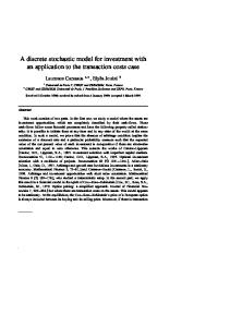
else set r = y ∗ ; find optimal r and update c∗2 (Propositions 5, 6) endif (4) update c∗ = min{c∗1 , c∗2 } and policy (r, S1 , S2 ) e 2 ) ≤ c − ϕ1 L(y ∗ ) if S2 = y ∗ or ϕ2 L(S then increase S2 by 1 and go to (1) (Proposition 8) If h > ϕ1 (p1 − p2 ), the upper bound in Proposition 8, along with other properties, ensures that the above algorithm finds an optimal policy in finite time. Now let us turn our attention to the case h < ϕ1 (p1 − p2 ), in which the upper bound in Proposition 8 is not valid. In this case, we implement a heuristic but effective (as shown in the next section) algorithm with one natural upper bound. For each S2 , the optimal costs, say c∗1 (S2 ), c∗2 (S2 ), are computed. Let us denote the minimum of the two by c∗ (S2 ). Now, consider the traditional (s, S) model which takes the quotation cost as its order setup cost. Its optimal cost is written as c∗s . To compute this value, the algorithm in Zheng and Federgruen (1991) can be used for instance. Since any (s, S) policy is a special case of (r, S1 , S2 )-type policies, we clearly have a well-defined value V = sup {S2 : c∗ (S2 ) ≤ c∗s } . If V is finite and −c∗ (·) is uni-modular, it will take only finite steps to search for the best c∗ . Although such properties are not rigorously confirmed in this paper, we still utilize this property and call it Algorithm II. Two algorithms are identical except for the last step. In the second one, the process of searching upwards for better S2 continues while c∗ (S2 ) is decreasing or it is increasing but less than c∗s . Some restrictions on the number of iterations can be imposed as well to ensure the termination of the algorithm in a finite number of steps. This approach turns out to work well for the test cases in the next section. Interestingly, the cost savings are more significant when h < ϕ1 (p1 − p2 ) than the other.

5. Numerical Studies We generate 135 instances to test the proposed algorithms, in all of which we have h = 2, and demands follow a Poisson distribution with mean µ = 10. Since it is p1 − p2 rather than p1 or p2 alone that affects the cost functions (4) and (6), we fix p2 = 0 and assign positive values to p1 , say p1 ∈ {1, 3, 5}. Other values used in the numerical studies include Q ∈ {1, 5, 10, 20, 30}, b ∈ {10, 20, 30}, and ϕ1 ∈ {0.1, 0.4, 0.7}. We impose Assumption 1 when we set the values for b, whereas we consider two possibilities for h: h > ϕ1 (p1 − p2 ) and h < ϕ1 (p1 − p2 ). Of the 135 instances, 90 of them have h > ϕ1 (p1 − p2 ), which are to be solved by Algorithm I, and 45 instances are with h < ϕ1 (p1 − p2 ), which are solved by Algorithm II. All tests are implemented in MATHEMATICA Version 5.1 on a Pentium 4 computer running Windows 20

Algorithm I

Algorithm II

45

7

40

6

number of instances

number of instances

35 30 25 20 15

5 4 3 2

10 1

5 0

1

1.5

2

2.5

3 time (sec)

3.5

4

4.5

0

5

1.4

1.6

1.8 time (sec)

2

2.2

2.4

Figure 1: Histograms of computational time: (left) h > ϕ1 (p1 − p2 ) (right) h < ϕ1 (p1 − p2 ). XP with 2.4GHz CPU and 512 MB memory. In every test instance, optimization algorithms successfully locate the optimal solution which is verified by an exhaustive search algorithm. The performance of the algorithms can be checked in terms of computational efficiency, cost saving, and optimality. For each test case, the renewal and discounted renewal functions m(i), m(i), mϕ1 (i), mϕ1 (i), M (i), M (i), Mϕ1 (i), M ϕ1 (i) are initially computed up to i = 90 and stored for later use. The mismatch cost function L(y) is computed for y from −90 to 90 and stored as well. The total running times include such offline computations. We observe from the numerical results (Figure 1) that it takes typically around one to several seconds to complete computations while the exhaustive search may take from several minutes up to hours depending on how far S2 is searched upwards. As for cost saving, we compare the results with the classical inventory model with (s, S) policies and with 3-parameter policies r < S1 ≤ S2 which are natural extensions of (s, S) policies (e.g., Kalymon, 1971). Here, we compute the optimal (s, S) policies for the same test cases, following the algorithm of Zheng and Federgruen (1991) and treating Q as the order setup cost. The results are reported in Figure 2. In all cases considered, each optimal (r, S1 , S2 ) policy costs less than or equal to the optimal (s, S) policy, thanks to the additional flexibility of ordering up to different levels upon different quoted prices. In some cases, the percentage of cost saving is as large as 50%. The numerical study of 3-parameter policies show the effectiveness of speculative ordering decisions. There are 25 relevant instances in the test cases such that optimal policies are found in W1 . For these cases, the exhaustive search finds optimal 3-parameter policies and Figure 3 summarizes the results, showing nontrivial percentage savings. Lastly, we numerically test the optimality of the proposed policies and the algorithms. The optimal costs for all cases are derived based on the value iteration algorithm as explained in Puterman (1994). Since the state space in our model is not bounded, we truncate the state space to a finite interval [sl , su ] where sl and su are set up to −300 and 300, respectively. Total up to 45 iterations are enough to induce convergence in

21

Algorithm I

Algorithm II

20

6

18 5

14

number of instances

number of instatnces

16

12 10 8 6 4

4

3

2

1

2 0

0

5

10

0

15

cost saving (%)

10

15

20

25

30 35 cost saving (%)

40

45

50

55

Figure 2: Histograms of cost saving: (left) h > ϕ1 (p1 − p2 ) (right) h < ϕ1 (p1 − p2 ). the increments of the value functions. We then observe that the proposed policies and algorithms correctly find the optimal costs in all of the test cases. Before concluding this section, we make additional observations regarding two questions; (1) when does it help to have a speculative inventory policy? and (2) how is the percentage cost saving related to parameter values? As for the first one, we note that, out of total 135 test cases, there are 106 cases where the optimal policy is in set V1 with r < S1 ≤ y1∗ ≤ S2 , and there are 4 cases in V2 with r < y1∗ < S1 ≤ S2 . For these cases, recall that an order will always be placed once a quote is requested. On the other hand, the remaining 25 cases have optimal policies in set W1 with S1 ≤ r < S2 and y ∗ ≤ r. In such cases, it is optimal to request a quote speculatively, i.e., a quote is requested to see if a low price is available. These cases have relatively small Q values, which is consistent with the intuition that speculative quotation is worth doing only if the incurred cost is low compared with the potential saving from ordering only at a low price. It should be noted that there is not a single case which has an optimal policy in set W2 , which verifies the claim of Proposition 7 numerically. On the other hand, except for just a few cases, optimal order-up-to levels S1 and S2 are different, yielding non-zero cost savings. Moreover, this percentage cost saving tends to be large as is ϕ1 (p1 − p2 ). See Figure 4 for an illustration. One natural explanation would be that an optimal policy with additional flexibility saves more if there is a big expected cost difference between quoted prices. This provides an answer to the question (2) above. One last remark is made on the heuristic upper bound in Algorithm II. At the end of the previous section, we mentioned that one requirement to guarantee the termination of the algorithm in finite time is the uni-modularity of −c∗ (·). Our numerical experiments show that there exist cases that the function is not uni-modular. But, it turns out that all the test cases with h < ϕ1 (p1 − p2 ) have uni-modular −c∗ (·), which might deserve further investigation in the future.

22

3−parameter heuristic policy

Algorithm I

10

15

9

7

cost saving (%)

number of instances

8

6 5 4

10

5

3 2 1 0

0

2

4 6 cost saving (%)

8

0

10

0

0.2

0.4

0.6 0.8 φ1(p1−p2)

1

1.2

1.4

Figure 4: Scatter plot of ϕ1 (p1 − p2 ) versus cost saving.

Figure 3: Histogram of cost saving compared to a 3-parameter policy.

6. Concluding Remarks This paper combines price search, a basic feature of the economic markets, and inventory management with stochastic demand. As an inventory model, ours is simplified as the traditional order setup cost is assumed zero, but still an extension in that the price search cost is explicitly formulated, which plays the role of the setup cost. As a price search problem, our model is limited in that it assumes only two prices and the price search is just a “go/no-go” decision. However, it is an extension as it considers stochastic demands over an infinite horizon. Our focus is on optimizing (r, S1 , S2 )-type policy using the developed algorithms based on structural properties we have identified. The proposed policy result in significant cost savings up to 50% over the naive application of the classical (s, S) policy in the numerical studies. We, in addition, have observed the effectiveness of the speculative buying decisions through numerical tests by considering certain 3-parameter policies. The optimality of the proposed policy is unknown, although the (r, S1 , S2 )-type policy has been found to be optimal numerically in all the cases presented in this paper. The (r, S1 , S2 )-type policy may not be optimal as we found a counter-example with a finite horizon (see Appendix A). The model can be extended in other directions as well. Firstly, the number of possible prices can be extended to n, which will subsequently extend the policy type to (r, S1 , S2 , · · · , Sn ). The total cost function for the case r < S1 ≤ S2 ≤ · · · ≤ Sn can be derived easily like the cost function for the case r < S1 ≤ S2 . However, the total cost functions for other cases will be much more complicated. Secondly, we can formulate the quotation process as an optimal stopping problem, adding an extra complexity due to the sequential search. This is interesting because of the obvious trade-off between a possible lower price versus the increased total search cost. Lastly, a study of effective policies when these problems are considered in a finite horizon should be intriguing as it poses different kinds of analytical challenges.

23

Acknowledgement The authors are grateful for many helpful and constructive comments from the anonymous referees, the Associate Editor, Prof. Dada (the Department Editor), and Prof. Yano (the Editor) that have been essential to improve the manuscript. The work of K. Kim was supported by the Basic Science Research Program through the National Research Foundation of Korea (NRF) funded by the Ministry of Education, Science and Technology (MEST, No. 2011-0007651).

References Albrecht, J., P. A. Gautier, S. Vroman. 2006. Equilibrium directed search with multiple applications. Review of Economic Studies 73(4) 869–891. Arrow, K. J., T. Harris, J. Marschak. 1951. Optimal inventory policy. Econometrica 19(3) 250–272. Bakos, J. Y. 1997. Reducing buyer search cost: Implications for electronic marketplaces. Management Science 43(12) 1676–1692. Chaouch, B. A. 2007. Inventory control and periodic price discounting campaigns. Naval Research Logistics 54(1) 94–108. Fabian, T., J. L. Fisher, M. W. Sasieni, A. Yardeni. 1959. Purchasing raw material on a fluctuating market. Operations Research 7(1) 107–122. Feng, Y., J. Sun. 2001. Computing the optimal replenishment policy for inventory systems with random discount opportunities. Operations Research 49(5) 790–795. Goh, M., M. Sharafali. 2002. Price-dependent inventory models with discount offers at random times. Production and Operations Management 11(2) 139–156. Golabi, K. 1980. An inventory model with search for best ordering price. Naval Research Logisitics Quarterly 27(4) 645–658. Hall, G., J. Rust. 2007. The (S, s) policy is an optimal trading strategy in a class of commodity price speculation problems. Economic Theory 30(3) 515–538. Kalymon, B. A. 1971. Stochastic prices in a single-item inventory purchasing model. Operations Research 10(6) 1434–1458. Magirou, V. F. 1982. Stockpiling under price uncertainty and storage capacity constraints. European Journal of Operational Research 11(3) 233–246. Moinzadeh, K. 1997. Replenishment and stocking policies for inventory systems with random deal offerings. Management Science 43(3) 334–342. 24

Nelson, R. 1995. Probability, Stochastic Processes, and Queueing Theory : The Mathematics of Computer Performance Modeling. Springer-Verlag, New York. ¨ Ozekici, S., M. Parlar. 1999. Inventory models with unreliable suppliers in a random environment. Annals of Operations Research 91(1) 123–136. Peleg, B., H. L. Lee, W. H. Hausman. 2002. Short-term E-procurement strategies versus long-term contracts. Production and Operations Management 11(4) 458–479. Porteus, E. L. 2002. Foundations of Stochastic Inventory theory. Stanford University Press, Palo Alto, CA. Puterman, M. L. 1994. Markov Decision Processes. Wiley, New Jersey. Ross, S. M. 2007. Introduction to Probability Models. 9th ed. Academic Press, New York. Scarf, H. 1960. The optimality of (s, S) policy in the dynamic inventory problem. K. J. Arrow, S. Karlin, P. Suppes, eds., Mathematical Methods in the Social Sciences, chap. 13. Stanford University Press. Tajbakhsh, M. M., C.-G. Lee, S. Zolfaghari. 2011. An inventory model with random discount offerings. Omega 39(6) 710–718. Teng, J.-T., H.-L. Yang. 2004. Deterministic economic order quantity models with partial backlogging when demand and cost are fluctuating with time. Journal of the Operational Research Society 55(5) 495–503. Veinott, A. F., H. M. Wagner. 1965. Computing optimal (s, S) inventory policies. Management Science 11(5) 525–552. Yang, H., L. Ye. 2008. Search with learning: understanding asymmetric price adjustments. RAND Journal of Economics 39(2) 547–564. Zheng, Y.-S. 1991. A simple proof for optimality of (s, S) policies in infinite-horizon inventory systems. Journal of Applied Probability 28(4) 802–810. Zheng, Y.-S. 1994. Optimal control policy for stochastic inventory systems with markovian discount opportunities. Operations Research 42(4) 721–738. Zheng, Y.-S., A. Federgruen. 1991. Finding optimal (s, S) policies is about as simple as evaluating a single policy. Operations Research 39(4) 654–665.

25

Appendix A The inventory problem we have studied can be formulated over a finite horizon as follows: { ft (x) = −λx + min Gt (λ, x), Q +

2 ∑

} ϕi min Gt (pi , y) y≥x

i=1

(10)

where t is the number of periods remaining, ft (x) is the value function at period t, Gt (p, y) = py + L(y) + αE[ft−1 (y − ξ)], and α is a discount factor. Although this is somewhat similar to the optimality equation in Porteus (2002), the argument does not apply as the minimizers of Gt (p, y) depend on the parameter p. Consider an example where there are three periods, demand follows an exponential distribution with mean 3, and f0 (·) = 0. The parameters used in the counter example are as listed in Table 3: Table 3: Model parameter values in the counterexample. p1 0.5

p2 4

ϕ1 6/7

ϕ2 1/7

h 0.1

b 10

E[ξ] 3

Q 15

α 0.9

In the example, G3 (p2 , ·) has two local minima, of which the smaller is the global minimizer. This means that if p2 is quoted the order-up-to policy is not optimal.

Appendix B Proof of Lemma 1. Part (a): We proceed as follows: for j ≥ 1,

α

j−1 ∑ k=0

mα (k)

∞ ∑

ψ(l) = α

l=j−k

j−1 ∑

mα (k) (1 − Ψ(j − k − 1))

k=0

= α

j−1 ∑

mα (k) − αΨ(j − 1) −

k=0

= αMα (j) − αΨ(j − 1) − = αMα (j) − αΨ(j − 1) −

∞ ∑ n=1 ∞ ∑

j−1 ∑ ∞ ∑

αn+1 ψ (n) (k)Ψ(j − k − 1)

k=0 n=1 j−1 ∑ n+1

α

ψ (n) (k)Ψ(j − k − 1)

k=0

αn+1 Ψ(n+1) (j − 1)

n=1

= αMα (j) −

∞ ∑

αn Ψ(n) (j − 1) = αMα (j) − Mα (j) + 1.

n=1

We used Mα (j) = 1 + M α (j − 1) = 1 +

∑∞

n=1 α

n Ψ(n) (j

26

− 1) in the last equality.

Part (b): We observe that, for j ≥ 1, j−1 ∑

∞ ∑

m(k)

k=0

=

(l + k)ψ(l) − µM (j)

l=j−k j−1 ∑

m(k)

k=0

 ∞ ∑ 

(l + k)ψ(l) −

l=j−k

∞ ∑ l=0

   j−1 j−k−1 ∞  ∑  ∑  ∑ lψ(l) = m(k) k ψ(l) − lψ(l) .    k=0

l=j−k

l=0

∑ ∑j−k−1 ∑j−1 It is easy to see that j−k−1 lψ(l) = (j − k)Ψ(j − k − 1) − l=0 Ψ(l), and k=0 km(k) = jM (j) − l=0 ∑j k=1 M (k). Then, straightforward calculations yield jM (j) −

j ∑

M (k) − j

k=1

j−1 ∑

m(k)Ψ(j − k − 1) +

k=0

j−1 ∑

m(k)

j−k−1 ∑

k=0

Ψ(l).

l=0

Now the following results are useful. j−1 ∑

m(k)Ψ(j − k − 1) = Ψ(j − 1) +

j−1 ∑ ∞ ∑

ψ (n) (k)Ψ(j − 1 − k)

k=0 n=1

k=0

= Ψ(j − 1) +

∞ ∑

Ψ(n+1) (j − 1) = M (j) − 1.

(11)

n=1

On the other hand, j−1 ∑ k=0

m(k)

j−k−1 ∑

Ψ(l) =

j−1 ∑ ∑

m(k)Ψ(l)

p=0 k+l=p

l=0

=

j−1 ∑

(M (p + 1) − 1) =

p=0

j ∑

M (p) − j

(12)

p=1

where we used (11) in the second equality. Plugging (11) and (12) into the original expression, then we obtain zero. Part (c): From direct computations,

α

j ∑

ψ(k)mα (j − k) = αψ(j) + α

k=0

j ∑

ψ(k)mα (j − k)

k=0

= αψ(j) + α

∞ ∑ n=1

= αψ(j) +

∞ ∑ n=1

27

αn

j ∑

ψ(k)ψ (n) (j − k)

k=0

αn+1 ψ (n+1) (j) = mα (j).

Part (d): Using Mα (0) = 0 and Mα (k) = 1 + M α (k − 1) for k ≥ 1, we have

α

j ∑

Mα (k)ψ(j − k) = α

k=0

= α

j ∑ k=1 j−1 ∑

{ 1+

∞ ∑

} n

α Ψ

(n)

(k − 1) ψ(j − k)

n=1

ψ(k) +

k=0

= αΨ(j − 1) +

∞ ∑ n=1 ∞ ∑

αn+1

j ∑

Ψ(n) (k − 1)ψ(j − k)

k=1

αn+1 Ψ(n+1) (j − 1) = Mα (j) − 1.

n=1

Proof of Lemma 2. Let S be the set of states that are reachable when the system starts from S1 or S2 . Then, from the system dynamics and the positive average demand, it is clear that the system with state space S is irreducible and positive recurrent. Therefore, there exists a stationary distribution P (·) from a standard theory of Markov chains. We can set P (j) = 0 if j ∈ / S. As a next step, we observe that P (·) satisfies the following relationships. For j > r, the state j is reachable from the previous period, say t − 1, when (1) xt−1 ≥ j and the demand size was xt−1 − j, and (2) xt−1 ≤ r, the lower price p2 was quoted, and the demand size was S2 − j. This can be written as P (j) = γϕ2 ψ(S2 − j) +

S2 ∑

P (k)ψ(k − j),

γ :=

r ∑

P (k).

k=−∞

k=j

Note that γ is the stationary probability that there is a quotation request in a period. This equation is that of (RE-3), and thus has a solution (with g(j) = γϕ2 ψ(S2 − j) and q = S2 ) P (j) =

S∑ 2 −j

γϕ2 ψ(S2 − j − k)m(k) = γϕ2 m(S2 − j)

k=0

where the second equality is from (c) of Lemma 1. Moreover,

1=

S2 ∑ j=−∞

P (j) = γ +

S2 ∑ j=r+1

 P (j) = γ 1 + ϕ2

S2 ∑



( ) m(S2 − j) = γ 1 + ϕ2 M (S2 − r − 1) .

j=r+1

By definition, 1 + ϕ2 M (S2 − r − 1) = ϕ1 + ϕ2 M (S2 − r), from which part (a) is immediate. Part (b) concerns with the case S1 < j ≤ r which does not exist if S1 = r. Similarly as above, let us consider each of possible scenarios. The state j is reachable if (1) xt−1 > r and the demand size was xt−1 − j, (2) xt−1 ≤ r, the lower price p2 was quoted, and the demand size was S2 − j, and lastly (3) j ≤ xt−1 ≤ r, the higher price p1 was quoted (hence no order), and the demand size was xt−1 − j. 28

Mathematically, it is

P (j) =

S2 ∑

P (k)ψ(k − j) + γϕ2 ψ(S2 − j) + ϕ1

k=r+1

r ∑

P (k)ψ(k − j).

k=j

∑ 2 Let us denote the first two terms by g(j) which is simplified to γϕ2 Sk=r+1 ψ(k − j)m(S2 − k). Then, ∑r−j again the above equation is of (RE-3) and thus P (j) = k=0 mϕ1 (k)g(j + k), which is exactly the formula in (b). Proof of (5). We first compute S2∑ −r−1

ψ(k)f (S2 − k) =

k=0

=

=

S2∑ −r−1

ψ(k)

S2 −k−r−1 ∑

k=0 S2∑ −r−1

∑

p=0

k+l=p

S2∑ −r−1

L(S2 − k − l)m(l)

l=0

L(S2 − p)ψ(k)m(l)

L(S2 − p)m(p)

p=0

=

S2∑ −r−1

L(S2 − p)m(p) − L(S2 ).

p=0

The third equality uses part (c) of Lemma 1. Let us write the first term in the last expression by Π. Then, it is immediate that C2 (j) = ϕ2 (p2 (S2 − j) + Π). Plugging this into EC and regrouping terms, we can see that EC = ϕ1 L(S1 ) + ϕ2 Π +

S1 ∑

Pe(j)ϕ1 p1 (S1 − j) +

+

Pe(j)ϕ2 p2 (S2 − j)

j=−∞

j=−∞ r ∑

r ∑

Pe(j)ϕ1 (L(j) − L(S1 )) + Q,

j=S1 +1

and the third, fourth terms can be re-written as S1 ∑ j=−∞

Pe(j)ϕ1 (p1 − λ)(S1 − j) +

r ∑

Pe(j)ϕ2 (p2 − λ)(S2 − j) + Υ

j=−∞

) ( ∑ ∑ 1 P (j)(S1 − j) + ϕ2 rj=−∞ P (j)(S2 − j) . Note that the expression in the with Υ = γ −1 λ ϕ1 Sj=−∞ parenthesis is the long-run average of order quantities per period. In the stationary system, this quantity must be equal to the expected demand per period; otherwise, the system accumulates infinite inventory or infinite back-orders. Therefore, Υ = γ −1 λµ. We also note that ϕ1 (p1 −λ) = ϕ1 ϕ2 (p1 −p2 ) = −ϕ2 (p2 −λ) 29

from λ = ϕ1 p1 + ϕ2 p2 . Putting these altogether and using

∑r

e

j=−∞ P (j)

= 1, it is not difficult to see that r ∑

EC = ϕ1 L(S1 ) + ϕ2 Π + ϕ1 ϕ2 (p2 − p1 )(S2 − S1 ) + γ −1 λµ + γ −1 ϕ1

( ) P (j) L(j) − L(S1 ) + Q

j=S1 +1

where L(j) − L(S1 ) = L(j) − L(S1 ) + ϕ2 (p1 − p2 )(j − S1 ) from the definition of L(·). As a last step, we use part (b) of Lemma 2. For the summation, it is equal to r ∑

) ( P (j) L(j) − L(S1 )

j=S1

=

r−j r ∑ ∑

( mϕ1 (k) γϕ2

j=S1 k=0

= γϕ2

r ∑

S2 ∑

) m(S2 − l)ψ(l − j − k)

(

) L(j) − L(S1 )

l=r+1 r ∑

S2 ∑

( ) mϕ1 (k ′ − j)m(S2 − l)ψ(l − k ′ ) L(j) − L(S1 )

j=S1 k′ =j l=r+1 ′

= γϕ2

S2 r k ∑ ∑ ∑

( ) mϕ1 (k ′ − j)m(S2 − l)ψ(l − k ′ ) L(j) − L(S1 ) .

l=r+1 k′ =S1 j=S1

Adding this term to EC, the desired result is obtained. Proof of Lemma 3. First, consider the case r < S1 ≤ S2 . Let (ru , S1u , S2u ) be an optimal (r, S1 , S2 ) policy with the largest S2 , i.e., S2u = max{S2∗ : c1 (r∗ , S1∗ , S2∗ ) = min{r
= ϕ1

∑

S2u −ru −1

m(j)∆L(S1u − j) + ϕ2

j=0

∑

m(j)∆L(S2u − j).

j=0

Now, due to the assumption that S1u ≤ S2u < y2∗ , we have Siu − j < y2∗ for all 0 ≤ j ≤ Siu − ru − 1 and for i = 1, 2. Since we have ∆L(y) ≤ 0 for y < y2∗ , the right side of the inequality is non-positive, and thus the claim is proved. However, this is a contradiction to the maximality of S2u . Let us turn to the second case, S1 ≤ r < S2 . Similarly as above, we define (ru , S1u , S2u ) where minimum of c2 (·) is taken over the set {S1 ≤ r < S2 }. Straightforwardly again, we obtain (c2 (ru + 1, S1u + 1, S2u + 1) − c2 (ru , S1u , S2u )) (ϕ1 + ϕ2 M (S2u − ru ))   S2u ru k ∑ ∑ ∑ = ϕ1 ∆L(S1u ) 1 − ϕ2 m(S2u − j) ψ(j − k) mϕ1 (k − l) k=S1u

j=ru +1

30

l=S1u

S2u −ru −1

∑

+ϕ2

m(j)∆L(S2u − j)

j=0 u

S2 ∑

+ϕ1 ϕ2

r ∑

k ∑

u

m(S2u

− j)

ψ(j − k)

k=S1u

j=ru +1

mϕ1 (k − l)∆L(l).

l=S1u

The following fact is proved below: for any S1 ≤ r < S2 , S2 ∑

1 − ϕ2

m(S2 − j)

j=r+1

r ∑

k ∑

ψ(j − k)

k=S1

mϕ1 (k − l) > 0.

(13)

l=S1

Again using ∆L(y) ≤ 0 for y < y2∗ , if S2u < y2∗ , then (ru + 1, S1u + 1, S2u + 1) would be also optimal and this is a contradiction to the maximality of S2u . Hence, we have S2u ≥ y2∗ for this case as well. Proof of (13). For any S1 ≤ r < S2 , we have S2 ∑

1 − ϕ2

m(S2 − j)

j=r+1

r ∑ k=S1

S2 ∑

= 1 − ϕ2

mϕ1 (k − l)

l=S1

m(S2 − j)

j=r+1

k ∑

ψ(j − k) r ∑

ψ(j − k)Mϕ1 (k − S1 + 1)

k=S1

by definition of Mϕ1 (·). If we set t = S2 − S1 + 1, n = S2 − r, p = S2 − j, and q = k − S1 + 1, then the above expression becomes (using i = t − q and Mϕ1 (0) = 0) 1 − ϕ2

n−1 ∑

m(p)

p=0

= 1 − ϕ2

t−n ∑

ψ(t − p − q)Mϕ1 (q)

q=1 n−1 ∑

m(p)

p=0

= 1 − ϕ2

n−1 ∑ p=0

= 1 − ϕ2 = 1 − ϕ2

n−1 ∑

m(p)

 t−p ∑ 

ψ(t − p − q)Mϕ1 (q) −

q=0

t−p ∑

t−p ∑ q=t−n+1

ψ(t − p − q)Mϕ1 (q) + ϕ2

q=0

n−1 ∑ n−1 ∑

  ψ(t − p − q)Mϕ1 (q)  m(p)ψ(i − p)Mϕ1 (t − i)

p=0 i=p

m(p) (Mϕ1 (t − p) − 1) /ϕ1 + ϕ2

n−1 i ∑∑

p=0

i=0 p=0

n−1 ∑

n−1 ∑

m(p) (Mϕ1 (t − p) − 1) /ϕ1 + ϕ2

p=0

i=0

31

m(p)ψ(i − p)Mϕ1 (t − i)

m(i)Mϕ1 (t − i) − ϕ2 Mϕ1 (t)

where we used part (d) of Lemma 1 in the third equality, and part (c) of the same lemma together with definition of m(·) in the last equality. Now, rearranging terms, we get ) ( n−1 n−1 ∑ ϕ2 ∑ 1 Mϕ1 (t − p) 1 − ϕ2 Mϕ1 (t) + m(p) + ϕ2 m(p) 1 − ϕ1 ϕ1 p=0

= 1 − ϕ2 Mϕ1 (t) +

p=0

n−1 ϕ2 ∑ m(p) (1 − ϕ2 Mϕ1 (t − p)) . ϕ1 p=0

Moreover, recall that Mϕ1 (·) satisfies, for x ≥ 1, Mϕ1 (x) = 1 +

∞ ∑

ϕj1 Ψ(j) (x

− 1) ≤ 1 +

j=1

∞ ∑ j=1

ϕj1 =

1 . ϕ2

Since Mϕ1 (0) = 0, the above expression is clearly non-negative. Actually, it is necessarily strictly positive. If it were zero, then, for instance, Ψ(j) (t) = P(ξ1 + · · · + ξj ≤ t) = 1 for all j ≥ 1 where the ξi denote i.i.d. demand random variables. However, this conclusion is absurd because ξi is assumed to have positive mean, ∑ and thus ji=1 ξi diverges to infinity almost surely. Proof of Lemma 4. We prove part (a) only as part (b) can be treated in a similar fashion. As in the proof of Lemma 3, we write (rl , S1l , S2l ) for an optimal policy with the smallest r, i.e., rl = min{r∗ : c1 (r∗ , S1∗ , S2∗ ) = min{r
c1 (rl , S1l , S2l ) − c1 (rl − 1, S1l − 1, S2l − 1)

)(

S1l −rl −1

= ϕ1

∑

) ϕ1 M (S1l − rl ) + ϕ2 M (S2l − rl )

S2l −rl −1

m(j)∆L(S1l − j − 1) + ϕ2

j=0

∑

m(j)∆L(S2l − j − 1).

j=0

We note that ∆L(y) ≥ 0 for all y ≥ y1∗ by the definition of y1∗ . Suppose that rl ≥ y1∗ . Then, ∆L(S1l − j − 1) ≥ 0 for any j = 0, . . . , S2l − rl − 1. This implies that (rl − 1, S1l − 1, S2l − 1) is also optimal and this is a contradiction to the definition of rl . Therefore, rl > y1∗ . Proof of Lemma 5. For part (a), we simply note that ∆L(y) = L(y + 1) − L(y) = −b + (b + h)Ψ(y) ↑ h, ∆2 L(y) = ∆L(y + 1) − ∆L(y) = (b + h)ψ(y + 1) ≥ 0. Since ∆L(y) = ∆L(y) + ϕ2 (p1 − p2 ) and ∆2 L(y) = ∆2 L(y), it is clear that L(·) is convex, and that ∆L(y) = −b + ϕ2 (p1 − p2 ) for any y < 0 and ∆L(y) > 0 for all sufficiently large y. 32

Suppose now that y ∗ > y1∗ . Then, L(y ∗ − 1) > L(y ∗ ) by definition of y ∗ . However, ∆L(y ∗ − 1) = ∆L(y ∗ − 1) + ϕ2 (p1 − p2 ) ≥ ϕ2 (p1 − p2 ) > 0. Since this is contradictory, we conclude that y ∗ ≤ y1∗ . As for the second statement of part (a), observe that if b > ϕ2 (p1 − p2 ), then L(·) is strictly decreasing in (−∞, 0) and thus y ∗ is finite. If b ≤ ϕ2 (p1 − p2 ), then L(·) is nondecreasing, leading to y ∗ = −∞. A proof of part (b) is based on straightforward calculations, but more involved. First, by a change of variable, we have b L(y) = ϕ2

∗ y−y ∑

( ) mϕ1 (k) L(y − k) − L(y ∗ ) − ϕ2 (p1 − p2 )y + L(y ∗ ),

k=0

which in turn yields b ∆L(y) = ϕ2

∗ y−y ∑

mϕ1 (k)∆L(y − k) − ϕ2 (p1 − p2 ).

(14)

k=0

Using this formula, we arrive at 2b

∗

∗

∆ L(y) = ϕ2 mϕ1 (y + 1 − y )∆L(y ) + ϕ2

∗ y−y ∑

mϕ1 (k)∆2 L(y − k) ≥ 0,

k=0

b is convex. Here, we used that L(·) is minimized at y ∗ and that L(·) is convex. On the which means that L(·) other hand, from (14), b ∆L(y) = ϕ2

∗ y−y ∑

mϕ1 (k)∆L(y − k) + ϕ22 (p1 − p2 )Mϕ1 (y + 1 − y ∗ ) − ϕ2 (p1 − p2 )

k=0

≤ ϕ2 Mϕ1 (y + 1 − y ∗ )∆L(y) + ϕ22 (p1 − p2 )Mϕ1 (y + 1 − y ∗ ) − ϕ2 (p1 − p2 ) = ∆L(y) (ϕ2 Mϕ1 (y + 1 − y ∗ ) − 1) + ∆L(y), where we used ∆L(·) is nondecreasing in the inequality. Since Mϕ1 (·) ≤ b for y ≥ y ∗ , we conclude that ∆L(y) ≤ ∆L(y) for any y ≥ y ∗ .

∑∞

j j=0 ϕ1

= 1/ϕ2 and ∆L(y) ≥ 0

To show yb∗ is finite and not smaller than y2∗ , we assume that yb∗ < y2∗ . Then, by definition of yb∗ , b y ∗ ) > 0. From the above result, this implies that ∆L(y ∗ − 1) ≥ ∆L(b b y ∗ ) > 0. This is then ∆L(b y ∗ ) ≥ ∆L(b 2 a contradiction to the definition of y2∗ . Hence, yb∗ ≥ y2∗ . We still need to prove that yb∗ is finite. To this end, consider (14). It was re-written as follows above: b ∆L(y) = ϕ2

∗ y−y ∑

mϕ1 (k)∆L(y − k) − ϕ2 (p1 − p2 ) (1 − ϕ2 Mϕ1 (y + 1 − y ∗ )) .

k=0

33

The second term is easily seen to converge to zero as y increases. On the other hand, the first term is greater than or equal to

∗ y−y ∑

ϕ2 mϕ1 (0)∆L(y) + ϕ2

mϕ1 (k)∆L(y − k),

k=y−y1∗

b using the nonnegativity of ∆L(y) for y ≥ y1∗ . It is clear that limk→∞ mϕ1 (k) = 0. Thus, limy→∞ ∆L(y) ≥ b ϕ2 mϕ (0)h = ϕ2 h/(1 − ϕ1 ψ(0)) > 0. Hence, L(y) is strictly increasing for all sufficiently large y, and 1

therefore yb∗ is finite. Proof of Lemma 6. For the first equality, we note that (α · c1 (r, S1 , S2 ) + (1 − α)L(r)) (ϕ1 M (S1 − r + 1) + ϕ2 M (S2 − r + 1)) = ϕ1

S1∑ −r−1

m(j)L(S1 − j) + ϕ2

S2∑ −r−1

j=0

m(j)L(S2 − j)

j=0

+ϕ1 ϕ2 (p2 − p1 )(S2 − S1 ) + (ϕ1 m(S1 − r) + ϕ2 m(S2 − r)) L(r) = ϕ1

S∑ 1 −r

m(j)L(S1 − j) + ϕ2

j=0

S∑ 2 −r

m(j)L(S2 − j) + ϕ1 ϕ2 (p2 − p1 )(S2 − S1 )

j=0

= c1 (r − 1, S1 , S2 ) (ϕ1 M (S1 − r + 1) + ϕ2 M (S2 − r + 1)) . Since M (x) > 0 for x ≥ 1 and non-decreasing in x, it is obvious that α ∈ (0, 1]. For the second inequality, we proceed as follows: (βc2 (S1 , S1 , S2 ) + (1 − β)L(S1 )) (ϕ1 M (1) + ϕ2 M (S2 − S1 + 1)) = ϕ1 L(S1 ) + ϕ2

S2 −S ∑1 −1

m(j)L(S2 − j) + Q + ϕ1 ϕ2 (p2 − p1 )(S2 − S1 )

j=0

+ (ϕ1 m(0) + ϕ2 m(S2 − S1 )) L(S1 ) = ϕ1 m(0)L(S1 ) + ϕ2

S∑ 2 −S1

m(j)L(S2 − j) + Q + ϕ1 ϕ2 (p2 − p1 )(S2 − S1 )

j=0

= c1 (S1 − 1, S1 , S2 ) (ϕ1 M (1) + ϕ2 M (S2 − S1 + 1)) . It is also clear that β ∈ (0, 1]. Proof of Lemma 7. It is obvious that γ ∈ (0, 1]. Now, let us consider the case: r + 1 < S2 . Recall that we have S1 = y ∗ ≤ r < S2 . To simplify notation, we set F (r, S1 , S2 ) =

S2 ∑ j=r+1

m(S2 − j)

r ∑

ψ(j − k)

k=S1

k ∑ l=S1

34

( ) mϕ1 (k − l) L(l) − L(S1 ) .

Then, from (6), c2 (r, S1 , S2 )(ϕ1 + ϕ2 M (S2 − r)) − c2 (r + 1, S1 , S2 )(ϕ1 + ϕ2 M (S2 − r − 1)) = ϕ2 m(S2 − r − 1)L(r + 1) + ϕ1 ϕ2 F (r, S1 , S2 ) − ϕ1 ϕ2 F (r + 1, S1 , S2 ) = ϕ2 m(S2 − r − 1)L(r + 1) S2 ∑

−ϕ1 ϕ2

m(S2 − j)ψ(j − r − 1)

j=r+1

r+1 ∑

) ( mϕ1 (r + 1 − l) L(l) − L(S1 )

(I)

l=S1

+ϕ1 ϕ2 m(S2 − r − 1)

r+1 ∑

ψ(r + 1 − k)

k=S1

k ∑

) ( mϕ1 (k − l) L(l) − L(S1 ) .

(II)

l=S1

As for (I), note that S2 ∑

m(S2 − j)ψ(j − r − 1) =

S2∑ −r−1

j=r+1

m(S2 − r − 1 − k)ψ(k) = m(S2 − r − 1)

k=0

where we used Lemma 1, part (c) in the second equality. Since r+1 < S2 , the right side is just m(S2 −r−1). For (II),

ϕ1

r+1 ∑

ψ(r + 1 − k)

k=S1

=

r+1 ∑

r+1 ∑

( ) mϕ1 (k − l) L(l) − L(S1 )

l=S1

{ ϕ1

r+1 ∑

}

ψ(r + 1 − k)mϕ1 (k − l)

(

) L(l) − L(S1 )

k=l

l=S1

=

k ∑

( ) mϕ1 (r + 1 − l) L(l) − L(S1 )

l=S1

=

r+1 ∑

) ( ) ( mϕ1 (r + 1 − l) L(l) − L(S1 ) − L(r + 1) − L(S1 ) .

l=S1

b + 1). Now, it is a simple Plugging these results into the original formula, we get ϕ2 m(S2 − r − 1)L(r algebra to get the desired expression. Let us turn our attention to part (b). When r + 1 = S2 , we have M (1) = m(0) by definition and thus c2 (r, S1 , S2 ) (ϕ1 + ϕ2 m(0)) = ϕ1 L(S1 ) + ϕ2 m(0)L(S2 ) + Q + ϕ1 ϕ2 (p2 − p1 )(S2 − S1 ) +ϕ1 ϕ2 m(0)

r ∑ k=S1

ψ(r + 1 − k)

k ∑ l=S1

35

) ( mϕ1 (k − l) L(l) − L(S1 ) .

(III)

The last term (III) can be simplified by observing that

ϕ1 ϕ2 m(0)

r+1 ∑

ψ(r + 1 − k)

k=S1

= ϕ1 ϕ2 m(0)

k ∑

( ) mϕ1 (k − l) L(l) − L(S1 )

l=S1 r+1 ∑ r+1 ∑

( ) ψ(r + 1 − k)mϕ1 (k − l) L(l) − L(S1 )

l=S1 k=l

= ϕ2 m(0)

r+1 ∑

) ( mϕ1 (r + 1 − l) L(l) − L(S1 )

l=S1

= ϕ2 m(0) {

r+1 ∑

) ( ) ( mϕ1 (r + 1 − l) L(l) − L(S1 ) − ϕ2 m(0) L(S2 ) − L(S1 )

l=S1

} ( ) b = m(0) L(S2 ) − L(S2 ) + L(S2 ) − L(S1 ) − ϕ2 m(0) L(S2 ) − L(S1 ) b in the last equality. where we used part (c) of Lemma 1 in the second equality and the definition of L(·) Similarly, we have ϕ1 ϕ2 m(0)ψ(0)

r+1 ∑

) ( mϕ1 (r + 1 − l) L(l) − L(S1 )

l=S1

{ } b 2 ) − L(S2 ) + L(S2 ) − L(S1 ) . = ϕ1 m(0)ψ(0) L(S Also, m(0)(1 − ψ(0)) = 1 by definition, and m(0)(1 − ϕ1 ψ(0)) = m(0) (ϕ1 (1 − ψ(0)) + ϕ2 ) = ϕ1 + ϕ2 m(0). Then, regrouping terms, we get c2 (r, S1 , S2 ) (ϕ1 + ϕ2 m(0)) b 2) = ϕ1 L(S1 ) + Q + ϕ1 ϕ2 (p2 − p1 )(S2 − S1 ) + m(0)(1 − ϕ1 ψ(0))L(S { } −ϕ1 m(0)(1 − ψ(0)) L(S2 ) − L(S2 ) + L(S1 ) b 2) = Q + ϕ1 ϕ2 (p2 − p1 )(S2 − S1 ) + (ϕ1 + ϕ2 m(0))L(S } { +ϕ1 L(S1 ) − L(S2 ) + L(S2 ) − L(S1 ) b 2 ). = Q + (ϕ1 + ϕ2 m(0))L(S Now, the result is immediate because γ = ϕ1 /(ϕ1 + ϕ2 m(0)). Proof of Proposition 7. First note that we can set an optimal S1o = r for fixed r and S2 thanks to Proposition 4. Let us write c2 (r) for c2 (r, r, S2 ) to simplify notation. A proof consists of several steps.

36

Step 1: We claim that there exists r < y ∗ such that c2 (r) ≤ L(r). We further claim that c2 (e r) ≤ L(e r) for any re ≤ r and this leads to c2 (e r) ≤ c2 (e r − 1). To show the first part, we observe from (6) that (c2 (r) − L(r)) (ϕ1 + ϕ2 M (S2 − r)) = ϕ2

S2∑ −r−1

m(j) (L(S2 − j) − L(r)) + Q + ϕ1 ϕ2 (p2 − p1 )(S2 − r).

j=0

Since L(y) is nonincreasing for y ≤ y1∗ and limy→−∞ L(y) = ∞, it is possible to choose r < y ∗ such that L(S2 − j) ≤ L(r) for any j = 0, . . . , S2 − r − 1. Taking a smaller r if necessary, we can make Q + ϕ1 ϕ2 (p2 − p1 )(S2 − r) ≤ 0. This proves the first claim. Let us fix such r. It is then enough to show c2 (r − 1) ≤ L(r − 1) for the second part, and this is based on the following computations: using M (S2 − r + 1) ≥ M (S2 − r), c2 (r) ≤ L(r), and the above equality, { } (c2 (r) − L(r)) − (c2 (r − 1) − L(r − 1)) (ϕ1 + ϕ2 M (S2 − r + 1)) ≥ ϕ2

S∑ 2 −r

m(j) (L(r − 1) − L(r)) − ϕ1 ϕ2 (p2 − p1 ),

j=0

which is nonnegative because L(y) is nonincreasing for y ≤ y1∗ and p1 > p2 . Now, for the last part, note the following relationship which is proved below: c2 (e r − 1) = δ · c2 (e r) + (1 − δ)L(e r) + Π

(15)

where δ = (ϕ1 +ϕ2 M (S2 − re))/(ϕ1 +ϕ2 M (S2 −e r +1)) and Π = −ϕ1 ∆L(e r −1)/(ϕ1 +ϕ2 M (S2 − re+1)). Indeed, c2 (r − 1) (ϕ1 + ϕ2 M (S2 − r + 1)) − c2 (r) (ϕ1 + ϕ2 M (S2 − r)) = ϕ1 L(r − 1) + ϕ2

−

m(j)L(S2 − j) + Q + ϕ1 ϕ2 (p2 − p1 )(S2 − r + 1)

j=0

  

S∑ 2 −r

ϕ1 L(r) + ϕ2

S2∑ −r−1 j=0

  m(j)L(S2 − j) + Q + ϕ1 ϕ2 (p2 − p1 )(S2 − r) 

= −ϕ1 ∆L(r − 1) + ϕ2 m(S2 − r)L(r) + ϕ1 ϕ2 (p2 − p1 ) = −ϕ1 ∆L(r − 1) + ϕ2 m(S2 − r)L(r). Then, we have, for re ≤ r such that c2 (e r) ≤ L(e r), c2 (e r − 1) − c2 (e r) = (1 − δ)(L(e r) − c2 (e r)) + Π ≥ Π

37

where we used that δ ∈ (0, 1] and the assumption that c2 (e r) ≤ L(e r). Now, since re < y ∗ , ∆L(e r − 1) ≤ 0 and thus Π ≥ 0. Therefore, we conclude that c2 (e r) ≤ c2 (e r − 1). Step 2: The previous step implies that rl = max {r < y ∗ : c2 (r) ≤ L(r)} is well defined and that c2 (rl ) ≤ c2 (r) for any r ≤ rl . Therefore, an optimal policy r∗ with r∗ ≥ rl exists for S1o = r∗ and for given S2 . In this step, we suppose that S2 > y ∗ . If c2 (y ∗ ) ≤ L(y ∗ ), then the policy (y ∗ , y ∗ , S2 ) ∈ W1 is at least as good as any policy in W2 . Indeed, nothing prevents us from extending the previous arguments in Step 1 to the region {r ≤ y ∗ }. If c2 (y ∗ ) > L(y ∗ ), then we claim that c2 (r) ≥ c1 (r, r + 1, S2 ) for r = rl , . . . , y ∗ − 1, which implies that we do not need to search W2 for an optimal policy in this case. By the assumption and the definition of rl , we have c2 (r + 1) > L(r + 1) for any r in the set {rl , . . . , y ∗ − 1}. Now, part (b) of Lemma 6 tells us c1 (r, r + 1, S2 ) = β · c2 (r + 1) + (1 − β)L(r + 1),

β=

ϕ1 + ϕ2 M (S2 − r − 1) . ϕ1 M (1) + ϕ2 M (S2 − r)

It is clear that β ≤ δ in (15) with re = r + 1. Observe c1 (r, r + 1, S2 ) = β (c2 (r + 1) − L(r + 1)) + L(r + 1) ≤ δ (c2 (r + 1) − L(r + 1)) + L(r + 1) = c2 (r) − Π where we utilized (15) and Π = −ϕ1 ∆L(r)/(ϕ1 + ϕ2 M (S2 − r)). Since r + 1 ≤ y ∗ , Π ≥ 0 and thus we conclude that c1 (r, r + 1, S2 ) ≤ c2 (r). Step 3: The last step deals with the remaining case: S2 = y ∗ . Recall that we have c2 (rl ) ≤ c2 (rl − 1) ≤ · · · with rl < S2 . Consider r = rl , . . . , S2 − 1. If r + 1 < S2 , then Lemma 6 is applicable and we have c2 (r + 1) > L(r + 1). Hence, the arguments in Step 2 imply that c1 (r, r + 1, S2 ) ≤ c2 (r). Finally, we consider the case r = S2 − 1. We will show that the same conclusion holds by direct computations. By the constraint S2 ≥ y2∗ , the assumption S2 = y ∗ means that y ∗ = y1∗ = y2∗ . Note that (c2 (r) − c1 (r, r + 1, r + 1))m(0)(ϕ1 + ϕ2 m(0)) = m(0) {ϕ1 L(r) + ϕ2 m(0)L(r + 1) + Q + ϕ1 ϕ2 (p2 − p1 )} − (ϕ1 + ϕ2 m(0)) (m(0)L(r + 1) + Q) = ϕ1 m(0)L(r) − ϕ1 m(0)L(r + 1) + ϕ1 Q(m(0) − 1) + ϕ1 ϕ2 (p2 − p1 )m(0) = ϕ1 m(0) {L(r) − L(r + 1) + ϕ2 (p2 − p1 )} + ϕ1 Q(m(0) − 1) = −ϕ1 m(0)∆L(r) + ϕ1 Qm(0). And the last expression is nonnegative because r < y ∗ . The proof is now complete. Proof of Proposition 8. We consider two cases separately: (i) c∗1 ≤ c∗2 (ii) c∗1 > c∗2 .

38

Step 1: Choose any c ≥ c∗1 and denote an optimal policy by (r∗ , S1∗ , S2∗ ) ∈ V . Let us define an auxiliary ∑ function G(r, y) = Q + y−r−1 m(j)L(y − j) for y > r. Then, from (4), it is immediate to see that j=0 ( ) c1 (r, S1 , S2 ) ϕ1 M (S1 − r) + ϕ2 M (S2 − r) = ϕ1 G(r, S1 ) + ϕ2 G(r, S2 ) + ϕ1 ϕ2 (p1 − p2 )(S1 − S2 ), which is simplified to c1 (r, y, y)M (y − r) = G(r, y) when S1 = S2 = y > r. It can be shown that G(r, y) = L(y) + Q (1 − Ψ(y − r − 1)) +

y−r−1 ∑

ψ(j)M (y − r − j)c1 (r, y − j, y − j).

(16)

j=0

This equation is shown below. Now, thanks to (16) and c ≥ c∗1 , ( ) c∗1 ϕ1 M (S1∗ − r∗ ) + ϕ2 M (S2∗ − r∗ ) − ϕ1 ϕ2 (p2 − p1 )(S2∗ − S1∗ )   Si∗ −r∗ −1 2   ∑ ∑ ≥ ϕi L(Si∗ ) + Q (1 − Ψ(Si∗ − r∗ − 1)) + ψ(j)M (Si∗ − r∗ − j)c∗1   j=0 i=1 { } 2 ∑ = ϕi L(Si∗ ) + Q (1 − Ψ(Si∗ − r∗ − 1)) + (M (Si∗ − r∗ ) − 1) c∗1 . i=1

In the equality, the definition M (0) = 0 and part (d) of Lemma 1 are used. This leads us to c∗1

≥

2 ∑

{ ϕi

} L(Si∗ )

+ Q (1 −

Ψ(Si∗

∗

− r − 1))

+ ϕ1 ϕ2 (p2 − p1 )(S2∗ − S1∗ )

i=1

≥ ϕ1 L(S1∗ ) + ϕ2 L(S2∗ ) + ϕ1 ϕ2 (p2 − p1 )(S2∗ − S1∗ ). e ∗ ) which is clearly greater than or equal to However, the last expression is equal to ϕ1 L(S1∗ ) + ϕ2 L(S 2 ) ( −1 ∗ ∗ ∗ ∗ ∗ e e ϕ1 L(y ) + ϕ2 L(S ). Therefore, L(S ) ≤ ϕ c − ϕ1 L(y ) and this implies that S ∗ ≤ U (c∗ ). 2

2

2

2

1

1

Step 2: An optimal policy (r∗ , S1∗ , S2∗ ) is found to be in W in this case. Proposition 4 implies that we can set S1∗ = r∗ ∧ y ∗ . Then, in (5), note that the last term is nonnegative, and therefore, ( ) c∗2 ϕ1 + ϕ2 M (S2∗ − r∗ ) − ϕ1 ϕ2 (p2 − p1 )(S2∗ − S1∗ ) ≥

ϕ1 L(S1∗ )

S2∗ −r∗ −1

+ ϕ2

∑

m(j)L(S2∗ − j) + Q = ϕ1 (L(S1∗ ) + Q) + ϕ2 G(r∗ , S2∗ ).

j=0

As before, from (16), we have G(r∗ , S2∗ ) ≥ L(S2∗ ) + Q (1 − Ψ(S2∗ − r∗ − 1)) + (M (S2∗ − r∗ ) − 1) c∗1 . Plugging this into the above expression and rearranging terms, it is not difficult to see that ( ) c∗2 ϕ1 + ϕ2 M (S2∗ − r∗ ) 39

{ } ( ) e 2∗ ) + Q (1 − Ψ(S2∗ − r∗ − 1)) + (M (S2∗ − r∗ ) − 1) c∗1 . ≥ ϕ1 L(S1∗ ) + Q + ϕ2 L(S Applying the assumption c∗2 < c∗1 and collecting terms with c∗2 , we get { } ( ) e 2∗ ) + Q (1 − Ψ(S2∗ − r∗ − 1)) c∗2 ≥ ϕ1 L(S1∗ ) + Q + ϕ2 L(S e ∗ ) ≥ ϕ1 L(y ∗ ) + ϕ2 L(S e ∗ ). ≥ ϕ1 L(S1∗ ) + ϕ2 L(S 2 2 The same argument as in Case (i) yields the desired result. Step 3: Lastly, we show (16). The equation is equivalent to the recursive expression: ∞ ∑

G(r, y) = L(y) + Q

ψ(j) +

y−r−1 ∑

ψ(j)G(r, y − j).

j=0

j=y−r

Indeed, for the right hand side, we have

L(y) + Q

∞ ∑

ψ(j) +

y−r−1 ∑

j=y−r

= L(y) + Q

ψ(j)G(r, y − j)

j=0 ∞ ∑

ψ(j) +

y−r−1 ∑

j=y−r

= L(y) + Q +

j=0

= L(y) + Q +

ψ(j) Q +

y−r−1−j ∑

j=0

y−r−1 ∑ y−r−1−j ∑

y−r−1 ∑

{

} m(k)L(y − j − k)

k=0

ψ(j)m(k)L(y − j − k)

k=0

∑

ψ(j)m(k)L(y − i)

i=0 j+k=p

= L(y) + Q +

y−r−1 ∑

m(i)L(y − i) = Q +

y−r−1 ∑

m(i)L(y − i)

i=0

i=0

where we used part (c) of Lemma 1 in the fourth equality. The last expression is G(r, y).

40