1
Advances in Speech Transcription at IBM under the DARPA EARS Program Stanley Chen, Brian Kingsbury, Lidia Mangu, Daniel Povey, George Saon, Hagen Soltau and Geoffrey Zweig IBM T. J. Watson Research Center, Yorktown Heights, NY 10598
Abstract—This paper describes the technical and system building advances made in IBM’s speech recognition technology over the course of the DARPA Effective Affordable Reusable Speechto-Text (EARS) program. At a technical level, these advances include the development of a new form of feature-based Minimum Phone Error training (fMPE), the use of large-scale discriminatively trained full-covariance gaussian models, the use of septaphone acoustic context in static decoding graphs, and improvements in basic decoding algorithms. At a system building level, the advances include a system architecture based on cross-adaptation and the incorporation of 2100 hours of training data in every system component. We present results on English conversational telephony test data from the 2003 and 2004 NIST evaluations. The combination of technical advances and an order of magnitude more training data in 2004 reduced the error rate on the 2003 test set by approximately 21% relative - from 20.4% to 16.1% - over the most accurate system in the 2003 evaluation and produced the most accurate results on the 2004 test sets in every speed category. Index Terms— large-vocabulary conversational speech recognition, EARS, discriminative training, full covariance modeling, finite state transducer, Viterbi decoding
I. I NTRODUCTION Under the auspices of the DARPA Effective Affordable Reusable Speech-to-Text (EARS) program from 2002 to 2004, a tremendous amount of work was done in the speech community towards improving speech recognition and related disciplines. The work spanned multiple fields ranging from traditional speech recognition to speaker segmentation and sentence boundary detection, and included separate foci on the transcription of broadcast news and telephone conversations. Further, speech data from three languages was used: English, Arabic and Mandarin. Focusing specifically on speech recognition, the work included algorithmic advances, new system architectures, and the collection and processing of an order of magnitude more training data than was previously used. This paper describes the algorithmic and system building advances made specifically at IBM. This work focused on the recognition of English language telephone conversations, as represented by the data collected and distributed by the Linguistic Data Consortium (LDC) for the EARS and earlier HUB-5 programs (see Section III-A for a full description of the data sources). Though several different collection protocols were used, the bulk of the data was collected under the “Fisher” protocol by paying volunteers a modest amount to call a phonebank where they were connected with other volunteers and Work funded by DARPA grant NBCH203001-2
asked to discuss one of several dozen topics. Examples of topics are “health,” “relationships” and “terrorism.” The data collection process was designed to get a representative sample of American (U.S.) telephone-quality speech in terms of gender, race, geographic location, and channel conditions [1]. Since the data is conversational in nature, it is relatively challenging due to the presence of numerous mistakes, repairs, repetitions and other disfluencies. While the techniques described in this paper were developed in the context of transcribing English language telephone conversations, it is important to note that they are not specific to the language or task. The techniques we describe are based on, and extend, the general framework of Hidden Markov Models (HMMs), and the use of Gaussian Mixture Models (GMMs) as output distributions. These frameworks, and our extensions of them, are broadly applicable, and out techniques have since been readily applied to other tasks such as the transcription of Arabic news broadcasts. The main contributions of our work are: • A novel feature space extension of Minimum Phone Error Training [2] termed fMPE. This is a transformation of the feature-space that is trained to optimize the Minimum Phone Error (MPE) objective function. The fMPE transform operates by projecting from a very high-dimensional, sparse feature space derived from gaussian posterior probability estimates to the normal recognition feature space and adding the projected posteriors to the standard features. A system that uses fMPE+MPE training is more accurate than a system using MPE alone by approximately 1.4% absolute (6.7% relative), measured on the RT03 test set. • The use of a large, discriminatively trained full-covariance system. We developed an efficient routine for likelihood computation that enables the use of full-covariance gaussians in time-constrained systems. • Static decoding graphs that use septaphone (or, to use the Greek version, heptaphone) context 1 . • System combination through cross-adaptation instead of acoustic rescoring of lattices. A cascade of speakeradapted systems is used, with the output of one system being used to estimate the speaker-adaptive transforms for 1 We note that the use of the term heptaphone would ensure the consistent use of Greek terms for acoustic terminology and Latin terms for language modeling. However, for consistency with the prevailing practice of using the Latin term quinphone to denote 5-phone context, we use the Latin term septaphone to denote 7-phone context in this paper.
2
the next. Training of all system components using an order of magnitude more data than previously available - specifically, 2100 hours of data. To illustrate how these technology threads can be tied together into a complete speech recognizer, we further describe two representative systems we developed for the 2004 EARS evaluation sponsored by NIST. Both systems focused on the transcription of conversational telephony speech (CTS). The first system we describe is a real time (1xRT) system suitable for the offline analysis of audio recordings in commercial applications, and the second is a 10-times slower than real time (10xRT) system which indicates how low we can push the error rate in the absence of a significant time constraint. Both systems had the distinction of having the lowest error rates in their respective categories in this evaluation. The remainder of this paper is divided into two main sections: Section II focuses on the technology improvements as general techniques, and Section III describes the architecture and particulars of the IBM systems that were used in the 2004 EARS evaluations. •
II. T ECHNOLOGY A DVANCES This section describes the technological advances made at IBM. These fall into the categories of discriminative training, full covariance gaussian modeling, large-context search space representation with Finite State Acceptors (FSAs), and efficient decoding techniques. We are currently using three forms of discriminative training. Section II-A describes two traditional model-based forms of discriminative training, and section II-B presents a novel feature-based technique. Section II-C discusses full-covariance modeling; section II-D covers improved methods for building decoding graphs, and section II-E describes enhancements in the decoding algorithms themselves. A. Model-space discriminative training The first form of discriminative training is a space-efficient form of Maximum Mutual Information (MMI) training [3], [4], [5], [6]. In contrast to standard Maximum Likelihood (ML) training, MMI training attempts to maximize the mutual information between the words in the training data and the acoustic feature vectors. This mutual information is estimated as: P Pλ (w,a) D log Pλ (w)Pλ (a) P = D log PPλλ(a|w) (a) P (a|w) = D log P PPλλ(x)P λ (a|x) x
where D represents the set of training data; w the words of a particular training utterance, a the acoustics of the utterance, and λ the parameters of the acoustic and language models. This leads to updates of the gaussian means and variances, using statistics computed under two different assumptions. In the first or “numerator” case, the data is aligned to the states of a Hidden Markov Model (HMM) that represents all word sequences consistent with the known transcription (there may be multiple sequences due to, for example, the placement of silence). This
represents the “contribution” of the numerator in the objective function. The second set of statistics is computed by aligning the data to an HMM that represents all possible word sequences (analogous to decoding). This represents the contribution of the denominator of the objective function. In both cases, it is conceptually a soft alignment that results in a posterior probability for every HMM state at each time instance. After these statistics are computed, the gaussian means and variances are updated according to [6]: µ ˆi = σ ˆi2 =
θinum (x)−θiden (x)+Di µi γinum −γiden +Di θinum (x2 )−θiden (x2 )+Di (σi2 +µ2i ) γinum −γiden +Di
−µ ˆ2i
In these equations, µi is the mean of the ith gaussian mixture, σi2 is its variance, θi (x) and θi (x2 ) are the first and second order statistics of the data assigned to gaussian i, and γi is the count of the number of observations assigned to it. Di is a number computed on a per-gaussian basis so as to ensure positive variances. (This constraint leads to a quadratic equation, and the larger value of Di is used.) In MMI training, the main computational burden is the computation of the “denominator” statistics. The “numerator” statistics are exactly those computed in standard ML training. Theoretically, the denominator statistics require a soft alignment of each utterance to an HMM that represents all possible word sequences. One way of doing this is to approximate the set of all possible word sequences with the set represented by a lattice created by decoding a training utterance. This is the “standard” method, and has the advantage that the lattice can be used for many iterations. In the lattice-free or implicit-lattice MMI procedure [7], we simply use efficient decoding technology to do the full computation. The HMM representing all possible word sequences is constructed using Finite State Transducer (FST) technology (see Section II-D), and a forwards-backwards pass over this graph results in the necessary state-level posteriors. While each iteration of lattice-free MMI takes longer than a comparable pass of lattice-based MMI, the disk requirements of the lattice-free technique are much smaller, which is advantageous when working with a large training set [8]. For example, with 2100 hours of data, lattices occupy approximately 30 GB of disk space, and this along with network congestion is saved with our technique. The runtime is well below real time, typically 0.5xRT. The second form of traditional discriminative training is MPE [2], [9]. This process uses a lattice-based framework; due to the nature of the objective function, it is not straightforward to eliminate them. In our implementation, lattices with fixed state alignments were used. Novel features include: • training with a pruned bigram language model having about 150K bigrams instead of a unigram language model (the language model was built with a vocabulary of 50,000 words); • averaging of the statistics in the MPE training over four sets of acoustic and language model weights, with the acoustic weight being either 0.10 or 0.16 and the language model weight being either 1.0 or 1.6 (the standard weights
3
we use are 0.1 and 1.0; the other two were chosen without significant experimentation and gave about 2% relative improvement); • smoothing the sufficient statistics for MPE with statistics derived from MMI-estimated means and variances rather than the ML estimates normally used in I-smoothing [2]; • flooring of the variances in the update to the 20th percentile of the distribution of all variances in the appropriate dimension. We now turn to our main innovation in discriminative training, Feature-space Minimum Phone Error Training. B. Feature-space discriminative training: fMPE In addition to the traditional forms of discriminative training mentioned above, we have developed a novel form of discriminative modeling, fMPE. This is a global discriminatively trained feature projection which works by projecting very high dimensional features based on gaussian posteriors down to the normal feature space and adding them to the normal features. The gaussian posteriors are defined without reference to the decoding graph or language model and assume a uniform prior. If we denote the likelihood of the ith gaussian as li , its posterior pi is given by li pi = P k lk The algorithm is described in more detail below. 1) Objective Function: The objective function of fMPE is the same as that of MPE [2]. This is an average of the transcription accuracies of all possible sentences s, weighted by the probability of s given the model: PR P (1) FMPE (λ) = r=1 s Pλ (s|Or )A(s, sr ) where Pλ (s|Or ) is defined as the scaled posterior sentence κ ν r |s) P (s) probability Ppλp(O κ ν of the hypothesized sentence s, u λ (Or |u) P (u) λ are the model parameters, κ and ν are scaling factors and Or the acoustics of the r’th utterance. The function A(s, sr ) is a “raw phone accuracy” of s given the reference sr , which equals the number of phones in the reference transcription sr for utterance r minus the number of phone errors. 2) Feature projection in fMPE: In fMPE, the acoustic vector xt in each time frame is converted into a very highdimensional feature vector ht by taking posteriors of gaussians. ht is then projected down and added to the original features to make a new feature yt : yt = xt + Mht
(2)
The matrix M is trained using the MPE objective function from a zero start. It is necessary to add the original features xt in order to provide a reasonable starting point for the training procedure. 3) Training the projection: In fMPE, the feature projection (the matrix M) is trained using a gradient descent method. A batch method is used, requiring 4–8 iterations. After each iteration, the models are updated by one iteration of ML training on the updated features. The learning rates are set for each matrix
ML 22.1
MPE 20.6
fMPE 20.2
fMPE+MPE 19.2
TABLE I W ORD ERROR RATES ON RT03. 849 K DIAGONAL COVARIANCE GAUSSIANS WITH SEPTAPHONE CONTEXT (66.2M PARAMETERS )
element Mij using formulae that try to take into account the amount of training data available for each matrix element and the variance of the baseline output features for that dimension. The training procedure is described in [10]. In addition, some modifications are described in [11] which improve the robustness of the training setup. 4) Obtaining the gradient: The gradient descent on the matrix M requires differentiating the MPE objective function with respect to the change in parameters. This is straightforward. However, a so-called “indirect” term is added to this differential which reflects the fact that we intend to perform ML training on the features. The HMM parameters will change with the features; this is taken into account by differentiating the objective function with respect to the HMM means and variances; and using the dependence of the means and variances on the training features to obtain the indirect differential of the objective function with respect to the features. The necessity of the indirect differential can also be seen in light of the model space interpretation of fMPE given in [12]. This approach notes that an offset of all the feature vectors is identical, in the likelihood computations, to an equal but opposite offset of every gaussian mean. 5) High dimensional features: As mentioned above, the high dimensional features ht are based on posteriors of gaussians. In detail, the features used in the fMPE experiments were obtained as follows. First, the gaussians in the baseline HMM set were clustered using a maximum likelihood technique to obtain 100,000 gaussians. Note that, as reported in [11], this gives better results than simply training the gaussians as a general HMM on speech data. Then, on each frame, the gaussian likelihoods are evaluated and normalized to obtain posteriors for each gaussian between zero and one. The resulting vector is spliced together with vectors adjacent in time and with averages of such vectors to form a vector of size 700,000 as described in [10]. 6) Combination with MPE: fMPE trains the model parameters using the maximum likelihood (ML) criterion. Because it is desirable to combine fMPE with model space discriminative training, we train the fMPE features first, and then perform MPE training with the fMPE features. In [12], experiments were reported in which MPE training was done first, and then fMPE training was performed without any model update (and hence without the indirect differential). This appeared to make no difference to the final result. 7) Improvements from fMPE: Table I shows results on a speaker adapted system (SA-DC of Sec. III-D), and using the output of system SI-DC to esimate the speaker adaptive transforms (vocal tract length normalization and constrained model adaptation). fMPE reduces the word error rate by approximately 1.4% (6.7% relative) over the use of traditional MPE
4
SAT SAT-fMPE
ML 23.2 21.4
MMI 22.1 20.0
The computation of the argument to the exponent is computationally expensive — O(N 2 ), where N is the dimensionality, and this expense has hindered the adoption of this form of model. To improve the evaluation time, we based the likelihood computation on a Cholesky decomposition of the inverse covariance matrix, Σ−1 = U T U , where U is an upper-triangular matrix. Denoting x − µ by δ, and the ith row of U with Ui , the computation becomes X (x − µ)0 Σ−1 (x − µ) = (Ui · δ) × (Ui · δ)
TABLE II W ORD ERROR RATES ON RT03. 143 K FULL - COVARIANCE GAUSSIANS WITH QUINPHONE CONTEXT (106M PARAMETERS )
alone. In further experiments on multiple tasks, we have found that fMPE alone reliably gives more improvement than MPE alone. MPE applied on top of fMPE then always gives further improvement, although this is typically less than half what it would give prior to fMPE. 8) Comparison with other work; and further work: The feature transformation used in fMPE is the same as that used in SPLICE [13], which is a technique for noise robustness. SPLICE was originally trained using ML and intended for noise adaptation of models; recently an MMI version of SPLICE [14] has been reported which works in the same situations as fMPE, i.e., normal training rather than adaptation. It gave good improvements on matched test data but helped very little when testing in noise conditions different from those used for training. Something similar was observed in [15] when applying fMPE to a digit-recognition task: it gave good improvements on matched noise conditions but very little on mismatched noise conditions. As mentioned above, a model-space formulation of fMPE was presented in [12]. This formulation allows an extension: fMPE corresponds to a shift in the means, but then a scale on the model precisions was also trained, which was called pMPE. However, it was not possible to get very much further improvement from this innovation. More generally, fMPE may be compared to the increasingly successful neural-net-based methods (e.g. [16], [17]) which may be viewed as non-linear transformations of the input space. The two approaches represent quite different ways to train the non-linear transform, as well as different functional forms for the transformation, and it would be useful to try different combinations of these elements. C. Full Covariance Modeling One of the distinctive elements of IBM’s recently developed technology is the use of a large-scale acoustic model based on full-covariance gaussians [18]. Specifically, the availability of 2100 hours of training data (Section III-B) made it possible to build an acoustic model with 143,000 39-dimensional full-covariance mixture components. We have found that fullcovariance systems are slightly better than diagonal-covariance systems with a similar number of parameters, and, in addition, are beneficial for cross-adaptation. To construct and use these models, a number of problems were solved: • Speed of gaussian evaluation. The likelihood assigned to a vector x is given by: 1 | 2πΣ |−1/2 exp(− (x − µ)0 Σ−1 (x − µ)) 2
i
•
This is the sum of positive (squared) quantities, and thus allows pruning a mixture component as soon as the partial sum across dimensions exceeds a threshold. Second, we used hierarchical gaussian evaluation as described in Section II-E.5. By combining these two approaches, the run time for full decoding was brought from 10xRT to 3.3xRT on a 3GHz Pentium 4 without loss in accuracy. Of this, approximately 60% of the time is spent in likelihood computations and 40% in search. The likelihood computation itself is about twice as slow as with diagonal covariance gaussians. Discriminative training. The use of the accelerated likelihood evaluation, tight pruning beams and a small decoding graph made lattice-free MMI [7] possible; in the context of MMI training, we adjust the beams to achieve real time decoding. One iteration on 2000 hours of data thus takes slightly over 80 CPU days. The MMI update equations are multivariate versions of those presented in Section IIA; the means and the covariance matrices were updated as follows: µ ˆi =
θinum (x) − θiden (x) + Di µi γinum − γiden + Di
(3)
num 0 den 0 0 ˆ i = θi (xx ) − θi (xx ) + Di (µi µi + Σi ) − µ ˆi µ ˆ0i Σ γinum − γiden + Di (4) where the θ’s represent the mean and variance statistics for the numerator and the denominator. θ(x) is the sum of the data vectors, weighted by the posterior probability of the gaussian in a soft alignment of the data to the numerator or denominator HMM (as done in standard expectation maximization (EM) training [19]. Similarly, θ(xx0 ) is the sum of weighted outer products. γi is the occupancy count of the gaussian. Both θs and γs are of course summed over ˆ i is posiall time frames. Di is chosen to ensure that Σ tive definite and has a minimum eigenvalue greater than a predefined threshold. This is done by starting with a minimum value and doubling it until the conditions are met. In addition, two forms of smoothing were used: – I-smoothing [2]:
θinum (x)
←− θinum (x)(1 + τ /γinum )
θinum (xx0 ) ←− θinum (xx0 )(1 + τ /γinum ) θinum
←− γinum + τ (5)
5
– Off-diagonal variance smoothing: σkl ←− σkl
•
γ num , (γ num + ν)
∀k 6= l
(6)
In training, τ and ν were both set to 200 (on average, each gaussian received about 1000 counts). The effect of MMI is illustrated in Table II for both standard Speaker Adaptive Training (SAT) [7], [20] features and SAT-fMPE features. MLLR transform estimation. Only the on-diagonal elements of the covariance matrix were used to estimate MLLR transforms; this produced WER reductions of approximately 1% absolute (5% relative), in line with expectations.
D. Building Large-Context Decoding Graphs We frame the decoding task as a search on a finite-state machine (FSM) created by the offline composition of several finitestate transducers (FSTs) [21], [22]. 2 Specifically, if we take G to be an FSM encoding a grammar or language model, L to be an FST encoding a pronunciation lexicon, and C to be an FST encoding the expansion of context-independent phones to context-dependent units, then the composition G ◦ L ◦ C yields an FST mapping word sequences to their corresponding sequences of context-dependent units. The resulting FSM, after determinization and minimization, can be used directly in a speech recognition decoder; such decoders have been shown to yield excellent performance [23], [24]. We note that while it is more common to perform the composition in the reverse direction (replacing each FST with its inverse), this computation is essentially equivalent and we view the mapping from high-level tokens to low-level tokens as more natural. While this framework is relatively straightforward to implement when using phonetic decision trees with limited context such as triphone decision trees, several computational issues arise when using larger-context trees. For example, with a phone set of size 45, the naive conversion of a septaphone decision tree to an FST corresponding to C above would contain 457 ≈ 3.7 × 10¹¹ arcs. Consequently, we developed several novel algorithms to make it practical to build large-context decoding graphs on commodity hardware. Whereas previous approaches to this problem focused on long-span left context [25], [26], our new methods approach the problem differently, and are able to handle both left and right context. With these algorithms, we were able to build all of the decoding graphs described in this paper on a machine with 6GB of memory. As an example of the gains possible from using larger-context decision trees, we achieved a gain of 1.6% absolute WER when moving from a quinphone system to a septaphone system. 1) Compiling Phonetic Decision Trees into FSTs: While the naive representation of a large-context phonetic decision tree is prohibitively large, after minimization its size may be quite 2 We use the term “finite state machine” to represent both finite state acceptors (FSAs) and finite state transducers (FSTs). Whereas acceptors represent weighted sets of symbol sequences, transducers represent mappings from sequences of input symbols to sequences of output symbols. Many operations can be made to work with either FSTs or FSAs, with no substantial difference. We use the term FSM in this section wherever the algorithms can use either FSTs or FSAs.
manageable. The difficulty lies in computing the minimized FST without ever needing to store the entirety of the original FST. In [27], we describe an algorithm for constructing the minimized FST without ever having to store an FST much larger than the final machine; this algorithm was first deployed for ASR in IBM’s 2004 EARS system. Briefly, we can express a finite-state machine representing the phonetic decision-tree as a phone loop FSM (a one-state FSM accepting any phone sequence) composed with a long sequence of fairly simple FSTs, each representing the application of a single question in the decision tree. By minimizing the current FSM after the composition of each FST, the size of the current FSM never grows much larger than the size of the final minimized machine. To prevent the expansion caused by the nondeterminism of FSTs encoding questions asking about positions to the right of the current phone, we use two different FSTs to encode a single question, one for positions to the left and one for positions to the right. When applying an FST asking about positions to the right, we apply the reversed FST to a reversed version of the current FSM, thereby avoiding nondeterministic behavior. For additional details, see [27]. In practice, we found that even with this process, we had difficulty compiling septaphone decision trees into FSTs for large trees. However, note that the final FST need not be able to accept any phone sequence; it need only be able to accept phone sequences that can be produced from the particular word vocabulary and pronunciation dictionary we are using. Thus, instead of starting with a phone loop accepting any phone sequence, we can start with a phone-level FSM that can accept the equivalent of any word sequence given our particular word vocabulary. For a septaphone decision tree containing 22K leaves, the resulting leaf-level FSM representation of the tree contained 337K states and 853K arcs. After grouping all leaves associated with a single phone into a single arc label and determinizing, the final tree FST had 3.1M states and 5.2M arcs. 2) Optimizing the Creation of the Full Decoding Graph: Even if the C graph can be efficiently computed, it is still challenging to compute a minimized version of G ◦ L ◦ C using a moderate amount of memory. To enable the construction of as large graphs as possible given our hardware constraints, we developed two additional techniques. First, we developed a memory-efficient implementation of the determinization operation, as detailed in [27]. This typically reduces the amount of memory needed for determinization as compared to a straightforward implementation by many times, with little or no loss in efficiency. This algorithm is used repeatedly during the graph expansion process to reduce the size of intermediate FSMs. Secondly, instead of starting with a grammar G expressed as an FST that is repeatedly expanded by composition, we begin with a grammar expressed as an acceptor, so that our intermediate FSMs are acceptors rather than transducers. That is, we encode the information that is normally divided between the input and output labels of a transducer within just the input labels of an acceptor, and we modify the transducers to be applied appropriately. This has the advantage that the determinization of intermediate FSMs can be done more efficiently.
6
AW
D
D AW AO G G AO G K
K EY
N-best degree Lattice link density
AE AE
JH
5 451.0
10 1709.7
TABLE III DOG
L ATTICE LINK DENSITY AS A FUNCTION OF N
FOR THE
DEV04 TEST SET.
T T
CAT
T EY T
2 29.4
ATE JH
D D
= emitting state
Speaker-adapted decoding LM rescoring + consensus
RT03 17.4 16.1
DEV04 14.5 13.0
RT04 16.4 15.2
AGED
TABLE IV = null state
W ORD ERROR RATES FOR LM
RESCORING AND CONSENSUS PROCESSING
ON VARIOUS
EARS
TEST SETS .
Fig. 1. Example of an FSA decoding graph (with phone labels instead of leaf labels).
E. Advanced Decoding Algorithms In the previous section, we have described how we create a fully flattened state-level representation of the search space in the form of an FSM. This section describes the use of these graphs in our Viterbi decoder, and the implementation “tricks” we use in that decoder. This material is covered under five topics: graph representation, the basic Viterbi search, lattice generation, search speed-ups, and the likelihood computation. 1) Graph Representation: The decoding graphs produced by the algorithms of the preceding section have three distinctive characteristics when compared to standard FSMs. The first characteristic is that they are acceptors instead of transducers. Specifically, the arcs in the graph can have three different types of labels: • leaf labels (context-dependent output distributions), • word labels, and • ² or empty labels (e.g., due to LM back-off states). Second, word labels are always placed at the end of a word, that is, directly following the corresponding sequence of leaves. This ensures that the time information associated with each decoded word can be recovered. In contrast, word labels in generic FSTs can be shifted with respect to the underlying leaf sequences, with the consequence that the output word sequences must be acoustically realigned to get correct word times and scores. The third characteristic has to do with the types of states present in our graphs: • emitting states for which all incoming arcs are labeled by the same leaf and • null states which have incoming arcs labeled by words or ². This is equivalent to having the observations emitted on the states of the graph and not on the arcs. The advantage of this is that the Viterbi scores of the states can be directly updated with the observation likelihoods and the scores of the incoming arcs. It can happen, however, that after determinization and minimization, arcs with different leaf labels point to the same emitting state. In this case, the state is split into several different states, each having incoming arcs labeled by the same leaf. Even when using large-span phonetic context, this phenomenon is relatively rare and leads to only a small increase in graph size
(<10%). Finally, each emitting state has a self-loop labeled by the leaf of the incoming arcs. Null states can have incoming arcs with arbitrary word or ² labels (but no leaf labels). An illustration of our graph format is given in Figure 1. It is important to note that while we represent the search space with an acceptor rather than a transducer, there is no loss in generality: it is a simple matter to turn a transducer with context-dependent phone units on the input side and words on the output side into an acceptor in which words and phones are interleaved. The converse mapping from acceptor to transducer is trivial as well. The main constraint that our technique does have is that word labels occur immediately after the last phone in a word. By allowing the word labels to move relative to the phone labels (as happens in some transducer operations), greater compaction could potentially be achieved in the minimization step, with the previously mentioned drawback that acoustic realignment would be necessary to recover the correct word-time information. 2) Viterbi search: At a high level, the Viterbi search is a simple token passing algorithm with no context information attached to the tokens. It can be written as an outer loop over time frames and an inner loop over sets of active states. A complication arises in the processing of null states that do not account for any observations: an arbitrary number of null states might need to be traversed for each speech frame that is processed. Furthermore, because multiple null-state paths might lead to the same state, the nulls must be processed in topological order. In order to recover the Viterbi word sequence, it is not necessary to store backpointers for all the active states. Instead one can store only the backpointer to the previous word in the sequence. More precisely, every time we traverse an arc labeled by a word, we create a new word trace structure containing the identity of the word, the end time for that word (the current time) and a backpointer to the previous word trace. We then pass a pointer to this trace as a token during the search. This procedure is slightly modified for lattice generation as will be explained later on. Storing only word traces rather than state traces during the forward pass reduces dynamic memory requirements dramatically (by several orders of magnitude for some tasks). The drawback of this technique is that the Viterbi state sequence cannot be recovered.
7 TIME
A CAT A DOG
t-1
3 1
THE CAT 4 ONE CAT 1
t
1
2
t
THE CAT
6
A CAT
4
t+1
ATE ATE
beam N in likelihood active states
THE CAT ATE 9 3
1x SI 10 75 5000
1x SA 12 100 15000
10x SI 14 200 15000
10x SA 14 200 15000
TABLE V
= Token
B EAM SETTINGS USED FOR SPEAKER - INDEPENDENT (SI) AND SPEAKER - ADAPTED (SA) DECODINGS UNDER DIFFERENT TIME
= Word trace
CONSTRAINTS .
1 X AND 10 X STAND FOR TIMES REAL - TIME .
Fig. 2. N-best lattice generation (N=2). Here arcs carry word labels and scores (higher scores are better). Word sequences are represented by hash codes. 32 on-demand hierarchical decoupled hierarchical on-demand
31.5 31 30.5 30 WER (%)
Even though we store minimal information during the forward pass, memory usage can be excessive for very long utterances, wide decoding beams, or lattice generation. To address this problem, we implemented garbage collection on the word traces in the following way. We mark all the traces which are active at the current time frame as alive. Any predecessor of a live trace becomes alive itself. In a second pass, the array of traces is overwritten with only the live traces (with appropriate pointer changes). When done every 100 frames or so, the runtime overhead of this garbage collection technique is negligible. 3) Lattice generation: The role of a lattice (or word graph) is to efficiently encode the word sequences which have appreciable likelihood given the acoustic evidence. Standard lattice generation in (dynamic search graph) Viterbi decoding uses a word-dependent N-best algorithm where multiple backpointers to previous words are kept at word ends [28], [29]. When using static graphs however, there is a complication due to the merges of state sequences that can happen in the middles of words. To deal with this, we adopt a strategy that is distinct from the earlier method of [30] in that we keep track of the N-best distinct word sequences arriving at every state. This is achieved by hashing the word sequences from the beginning of the utterance up to that state. More precisely, during the forward pass, we propagate N tokens from a state to its successors. Token i contains the forward score of the ith-best path, the hash code of the word sequence up to that point and a backpointer to the previous word trace. Once we traverse an arc labeled by a word, we create a new word trace which contains the word identity, the end time and the N tokens up to that point. We then propagate only the top-scoring path (token). At merge points, we perform a merge sort and unique operation to get from 2N to N tokens (the tokens are kept sorted in descending score order). This lattice generation procedure is illustrated in Figure 2. In Table III, we report the link density (number of arcs in the lattice divided by the number of words in the reference) as a function of N for the same pruning parameter settings. We normally use N=5 to achieve a good balance between lattice size and lattice quality. Table IV shows the word error rates for three different test sets obtained after language model rescoring and consensus processing of the lattices at the speaker-adapted level. The language model used to generate the lattices has 4.1M n-grams while the rescoring LM has 100M n-grams (Sec. III-B.2). 4) Search speed-ups: Here we present some search optimization strategies which were found to be beneficial. They are related with the way the search graph is stored and accessed and with the way pruning is performed.
29.5 29 28.5 28 27.5 27 26.5 0.1
0.2
0.3
0.4 0.5 0.6 Real-time factor (cpu time/audio time)
0.7
0.8
Fig. 3. Word-error rate versus real time factor for various likelihood schemes (EARS RT’04 speaker independent decoding). Times are measured on Linux Pentium IV 2.8GHz machines and are inclusive of the search.
•
•
•
Graph memory layout. The decoding graph is stored as a linear array of arcs sorted by origin state, each arc being represented by a destination state, a label and a cost (12 bytes/arc). Each state has a pointer to the beginning of the sequence of outgoing arcs for that state, the end being marked by the pointer of the following state (4 bytes/state). These data structures are similar to the ones described in [31]. Successor look-up table. The second optimization has to do with the use of a look-up table which maps static state indices (from the static graph) to dynamic state indices. The role of this table is to indicate whether a successor state has already been accessed and, if so, what entry it has in the list of active states. Running beam pruning. For a given frame, only the hypotheses whose score are greater than the current maximum for that frame minus the beam are expanded. Since this is an overestimate of the number of hypotheses which survived, the paths are pruned again based on the absolute maximum score for that frame (minus the beam) and a maximum number of active states (rank or histogram pruning). This resulted in a 10–15% speed-up over standard beam pruning.
5) Likelihood computation: In [24], we presented a likelihood computation strategy based on hierarchical gaussian evaluation that is decoupled from the search, and all the system results presented in this paper use that scheme. In this section, however, we present some speed-ups that come from combining the hierarchical evaluation method with “on-demand” like-
8
Name Fisher English Training Speech Part 1 Fisher English Training Speech Part 2 Fisher English Training Transcripts Part 1 Fisher English Training Transcripts Part 2 Switchboard I - Release 2 ISIP Transcripts, 25 Oct. 2001 Switchboard Cellular Part 1 Transcribed Audio Switchboard Cellular Part 1 Transcription CALLHOME American English Speech CALLHOME American English Transcripts Switchboard-2 Phase II Audio Switchboard-2 Phase III Audio Switchboard Cellular Part 1 Audio BBN/CTRAN Transcripts
LDC Catalog Number / Source LDC2004S13 LDC2005S13 LDC2004T19 LDC2005T19 LDC97S62 http://www.cavs.msstate.edu/hse/ies/projects/switchboard/index.html LDC2001S15 LDC2001T14 LDC97S42 LDC97T14 LDC99S79 LDC2002S06 LDC2001S13 Distributed by BBN to EARS participants TABLE VI
ACOUSTIC TRAINING DATA SOURCES AND AVAILABILITY.
Source HUB-4 Broadcast News
University of Washington Web Data
Name 1996 English Broadcast News Transcripts 1996 CSR Hub-4 Language Model 1997 English Broadcast News Transcripts UW 175M Word Distribution UW 191M Word Distribution UW 525M Word Distribution
Availability LDC97T22 LDC98T31 LDC98T28 Distributed by UW to EARS participants Distributed by UW to EARS participants Distributed by UW to EARS participants
TABLE VII L ANGUAGE MODEL TRAINING DATA SOURCES AND AVAILABILITY.
lihood computation where we evaluate the gaussians only for the states which are accessed during the search as suggested in [32]. This works as follows: first, we perform a top-down clustering of all the mixture components in the system using a gaussian likelihood metric until we reach 2048 clusters (gaussians). At run time, we evaluate the 2048 components for every frame and, for a given state accessed during the search, we only evaluate those gaussians which map to one of the top N (typically 100) clusters for that particular frame. Figure 3 shows the word error rate versus run-time factor (including search) for the three different likelihood schemes: “hierarchical decoupled” (pre-computation and storage of all the likelihoods), “on-demand” and “hierarchical on-demand” (computing ondemand only those gaussians which are in the most likely clusters). For both on-demand techniques, we use a batch strategy which computes and stores the likelihoods for eight consecutive frames, as described in [32]. To generate these curves, the beam settings were varied in equal increments from less restrictive to more restrictive values — from 200 to 50 in increments of 12.5 (rounded down) for the number of gaussian clusters evaluated; from 12 to 9 in increments of 0.25 for the beam, and from 10000 to 3000 in increments of 600 for the maximum number of states. The graph indicates that we improve the run time by approximately 20% at low error rates, when moving from uncoupled hierarchical computation to hierarchical on-demand computation. Table V shows the the beams used in our speaker-
independent and speaker-adapted systems; these were identified by manual tuning experiments. III. S YSTEMS This section describes the application of the previous techniques in specific systems. III-A describes the training data; III-B describes the details of the acoustic and language models; and III-C and III-D describe our 1xRT and 10xRT systems respectively. A. Training Data 1) Acoustic Model Data: The acoustic training set used audio and transcripts from five sources: Fisher parts 1–7, Switchboard-1, Switchboard Cellular, Callhome English, and BBN/CTRAN Switchboard-2. All the audio data are available from the LDC, http://www.ldc.upenn.edu, as are most of the transcripts. Details on the availability of each source are given in Table VI. The Fisher transcripts were normalized using a collection of 840 rewrite rules. 41 conversation sides in the original collection were rejected because they had insufficient quantities of data (less than 20 s. of audio), and an additional 47 hours of data containing words occurring 4 times or less in the whole corpus were rejected.
9
SWB BBN BN FSH UW191 UW175 UW525
Corpus Size, M Words 3.6 1.2 159 23 191 175 525
Count Cutoffs 0,0,0,0 0,0,0,0 0,0,1,1 0,0,0,0 0,0,1,1 0,0,1,1 0,0,1,1
Number of n-grams 4M 1.5M 65M 18M 62M 66M 144M
Perplexity on RT03 76.8 78.9 97.8 58.0 108 102 90.2
Weight in LM1 0.10 0.15 0.05 0.55 0.15 -
Weight in LM2 0.07 0.05 0.04 0.71 0.02 0.11
TABLE VIII L ANGUAGE MODEL CHARACTERISTICS FOR THE LM S BUILT FROM EACH DATA SOURCE , AND THEIR INTERPOLATION WEIGHTS IN THE COMPOSITE LM S . LM1 IS THE LM USED TO BUILD THE DECODING GRAPH , AND LM2
We used ISIP’s 25 October 2001 release of Switchboard transcripts for the Switchboard-1 data, with a few manual corrections of transcription errors. The BBN/CTRAN Switchboard-2 transcripts and LDC transcripts for Switchboard Cellular and Callhome English were normalized to follow internal conventions (e.g., spelling out acronyms and mapping all noise symbols to one for vocalized noises and one for all others), and a few manual corrections were made. In addition, the full collection of audio data was resegmented such that all training utterances had nominally 15 frames of silence at the beginning and end, and all single-word utterances were discarded [33]. This results in a small improvement in error rate (0.6% at the speaker-independent level). Following normalization, roughly 2100 hours of training data remained. 2) Language Model Data: The language model used all the acoustic data transcripts listed in Table VI, as well as broadcast news transcripts from the LDC and web data provided by the University of Washington [34]. These sources are listed in Table VII. B. System Basics We use a recognition lexicon of 30.5K words which was generated by extending our RT03 lexicon to cover the 5000 most frequent words in the Fisher data. The lexicon contains a total of 33K pronunciation variants (1.08 variants per word). Pronunciations are primarily derived from PRONLEX (LDC catalog number LDC9720 available at http://www.ldc.upenn.edu), with the manual addition of a few variants to cover reduced pronunciations that are common in conversational American English. Pronunciation variants have weights based on their unigram counts in a forced alignment of the acoustic training data. 1) Acoustic Modeling: The raw acoustic features used for segmentation and recognition are perceptual linear prediction (PLP) features as described in [24]. No echo cancellation was performed. The features used by the speaker-independent system are mean-normalized on a conversation side basis. The features used by the speaker-adapted systems are mean- and variancenormalized on a conversation side basis, but normalization statistics are accumulated only for frames labeled as speech in the speaker-independent pass.
IS THE RESCORING
LM.
Words are represented using an alphabet of 45 phones. Phones are represented as three-state, left-to-right HMMs. With the exception of silence and noise states, the HMM states are context-dependent, and may be conditioned on either quinphone or septaphone context. In all cases, the phonetic context covers both past and future words. The context-dependent HMM states are clustered into equivalence classes using decision trees. Context-dependent states are modeled using mixtures of either diagonal-covariance or full-covariance gaussians. For the diagonal-covariance systems, mixture components are allocated according to a simple power law, m = min(M, ceil(k × N 0.2 )), where m is the number of mixture components allocated to a state, M is the maximum number of mixtures allocated to any state, N is the number of frames of data that align to a state in the training set, and k is a constant that is selected to set the overall number of mixtures in the acoustic model. Initial maximum-likelihood training of the diagonal-covariance systems is based on a fixed, forced alignment of the training data at the state level [33], and uses an iterative mixture-splitting method to grow the acoustic model from a single component per state to the full size. Typically, maximum-likelihood training concludes with one or two passes of Viterbi training on word graphs. All training passes are performed over the full 2100-hour acoustic training set. In the context of speaker-adaptive training, we use two forms of feature-space normalization: vocal tract length normalization (VTLN) [35] and feature-space Maximum Likelihood Linear Regression (fMLLR, also known as constrained MLLR) [36]. This process produces canonical acoustic models in which some of the non-linguistic sources of speech variability have been reduced. The VTLN warping is implemented by composing 21 piecewise linear warping functions with a Mel filterbank to generate 21 different filterbanks. In decoding, the warping function is chosen to maximize the likelihood of the frames that align to speech under a model that uses a single, full-covariance gaussian per context-dependent state to represent the classconditional distributions of the static features. Approximate Jacobian compensation of the likelihoods is performed by adding the log determinant of the sum of the outer product of the warped cepstra to the average frame log-likelihood. When decoding, we do a single pass of MLLR adaptation for
10 Speech Speech/non-speech segmentation
0.01xRT
SI decoding
0.14xRT
VTLN
0.02xRT
FMLLR
Front-end
0.10xRT
Alignments
0.04xRT
SI ±2 7.9K 150K 32.9K 3.9M 18.5M 44.5M
SA ±3 21.5K 849K 32.9K 4.2M 26.7M 68.7M
0.02xRT
TABLE IX
0.03xRT
G RAPH STATISTICS FOR THE SPEAKER - INDEPENDENT (SI) AND SPEAKER - ADAPTED (SA) DECODING PASSES . T HE NUMBER OF ARCS
Total RTF MLLR
Phonetic context Number of leaves Number of gaussians Number of words Number of n-grams Number of states Number of arcs
0.92xRT
INCLUDES SELF - LOOPS .
SA decoding
0.55xRT
Words
Fig. 4. 1xRT system diagram. Dashed lines indicate that the fMLLR and MLLR steps rely on the 1-best output of the speaker independent decoding. Run times are reported on a Linux Pentium 4 3.4GHz, 2.0GB machine.
each conversation side, using a regression tree to generate transforms for different sets of mixture components. The regression tree is an 8-level binary tree that is grown by pooling all of the mixture component means at the root node, then successively splitting the means at each node into two classes using a soft form of the k-means algorithm. The MLLR statistics are collected at the leaves of the tree and propagated up the tree until a minimum occupancy of 3500 is obtained and a transform is generated. In addition to these speaker-adaptive transforms, we increase the discriminating power of the features through the use of Linear Discriminant Analysis (LDA) followed by a diagonalizing transform. The specific diagonalizing transform we use is referred to as both Semi-Tied Covariances (STC) [37] and Maximum Likelihood Linear Transforms (MLLT) [38], [39]. Both attempt to minimize the loss in likelihood incurred by the use of diagonal covariance gaussians as opposed to full covariance gaussians. 2) Language Modeling: The IBM 2004 system uses two language models: a 4.1M n-gram language model used for constructing static decoding graphs, and a 100M n-gram language model that is used for lattice rescoring. Both language models are interpolated back-off 4-gram models smoothed using modified Kneser-Ney smoothing. The interpolation weights are chosen to optimize perplexity on a held-out set of 500K words from the Fisher corpus. The characteristics of the constituent language models, as well as their interpolation weight in the decoding-graph and rescoring language models are given in Table VIII. The unigram through 4-gram count thresholds are given in the column entitled “Count Cutoffs.” A threshold of 0 means every n-gram was used, and a cutoff of 1 means only n-grams occurring at least twice were used.
C. 1xRT System Architecture The operation of our 1xRT system comprises the steps depicted in Figure 4: (1) segmentation of the audio into speech
and non-speech segments, (2) speaker independent (SI) decoding of the speech segments, (3) alignment-based vocal tract length normalization of the acoustic features, (4) alignmentbased estimation of one maximum likelihood feature space transformation per conversation side, (5) alignment-based estimation of one MLLR transformation per side and (6) speakeradapted (SA) decoding using MPE-SAT trained acoustic models transformed by MLLR. The decoding graphs for the two decoding passes are built using identical vocabularies, similarly sized 4-gram language models, but very different context decision trees: the SI tree has 7,900 leaves and quinphone context, while the SA tree has 21,500 leaves and septaphone context. Table IX shows various decoding graph statistics. The maximum amount of memory used during the determinization step was 4GB. The severe run-time constraints for the 1xRT system forced us to choose quite different operating points for the speakerindependent and speaker-adapted decoding. Thus, the SI decoding was allotted a budget of only 0.14xRT, while the SA decoding received 0.55xRT. This had an influence on the number of search errors (2.2% versus 0.3%). In Table X, we indicate various decoding statistics for the two passes. In this table, the first row, “Likelihood/search ratio” shows the percentage of the total runtime dedicated to likelihood computation and Viterbi recursions (search) respectively. The second row, “Avg. number of gaussians/frame,” shows the average number of gaussians whose likelihoods were computed for each frame, using the hierarchical likelihood computation (about 1/20th of the total for both the SI and SA decodings). The last row, “Max. number of active states/frame,” shows the cutoffs used in rank pruning. The memory usage for the resource-intensive SA decoding broke down into 1.2GB of static memory (divided into 932MB for the decoding graph and 275MB for 850K 40-dimensional diagonal covariance gaussians) and 133MB of dynamic memory (220MB with lattice generation). D. A 10xRT Cross-adaptation Architecture Our 10xRT system is organized around system combination through cross-adaptation. Like many evaluation systems [40], [41], [42], several different recognition systems are used in combination to produce the final output. While this is typically done by generating lattices with one system and rescoring them
11
Word error rate Likelihood/search ratio Avg. number of gaussians/frame Max. number of active states/frame
SI 28.7 60/40 7.5K 5K
SA 19.0 55/45 43.5K 15K
models/transcripts SA.FC SA.DC
SA.FC 21.9 21.0
SA.DC 21.2 21.4
TABLE XI
TABLE X
W ORD ERROR RATES ON RT03. C OMPARISON BETWEEN SELF - AND CROSS - ADAPTATION . A ROW / COLUMN ENTRY WAS GENERATED BY
D ECODING STATISTICS ON RT04 FOR THE 1 X RT SYSTEM .
ADAPTING THE ROW- SPECIFIED MODELS WITH TRANSCRIPTS FROM THE COLUMN - SPECIFIED SYSTEM .
with other systems, all communication in the 2004 IBM 10xRT architecture is done through cross-adaptation. Three different acoustic models were used in our 10xRT system. In the enumeration below and in later passages, each system is given a two-part name. The first part indicates whether it is speaker-independent or speaker-adapted (SI or SA), and the second part indicates whether it is a diagonal or full-covariance system (DC or FC). 1) SI.DC: A speaker-independent model having 150K 40dimensional diagonal-covariance mixture components and 7.9K quinphone context-dependent states, trained with MPE. Recognition features are derived from an LDA+MLLT projection from 9 frames of spliced, speaker-independent PLP features with blind cepstral mean normalization. 2) SA.FC: A speaker-adaptive model having 143K 39dimensional full-covariance mixture components and 7.5K quinphone context-dependent states, trained with MMI and fMLLR-SAT. Recognition features are derived from fMPE on an LDA+MLLT projection from 9 frames of spliced, VTLN PLP features with speech-based cepstral mean and variance normalization. 3) SA.DC: A speaker-adaptive model having 849K 39dimensional diagonal-covariance mixture components and 21.5K septaphone context-dependent states, trained with both fMPE and MPE, and fMLLR-SAT. Recognition features are derived from fMPE on an LDA+MLLT projection from 9 frames of spliced, VTLN PLP features with speech-based cepstral mean and variance normalization. The recognition process comprises the following steps: 1) Segmentation of the audio into speech and non-speech. 2) Decoding the speech segments with the SI.DC model. 3) Speaker adaptation and decoding with the SA.FC model: a) Estimation of speech-based cepstral mean and variance normalization and VTLN warping factors using the hypotheses from (2). b) Estimation of fMPE, fMLLR and MLLR transforms for the SA.FC model using the hypotheses from (2). c) Decoding with the SA.FC model. 4) Reestimation of MLLR transforms and decoding with the SA.DC model: a) Estimation of MLLR transforms using the features from (3b) and the hypotheses from (3c). b) Lattice generation with the SA.DC model. 5) Lattice rescoring with the 100M n-gram LM described in
SI.DC (Step 2 output) SA.FC (Step 3c output) SA.DC (Step 4b 1-best) SA.DC Final (Step 6 output)
RT03 28.0 19.7 17.4 16.1
DEV04 23.5 16.6 14.5 13.0
RT04 26.7 18.8 16.4 15.2
TABLE XII W ORD ERROR RATES AT DIFFERENT SYSTEM STAGES .
Section III-B.2. 6) Confusion network generation and the extraction of the consensus path [43]. The effect of cross-adaptation was studied on a combination of diagonal and full covariance models (Table XI). Adapting the DC models on the errorful transcripts of the FC system led to a gain of 0.4% compared with self adaptation. Word error rates at the different system stages are presented in Table XII for the 2003 test set provided by NIST, the 2004 development set, and the RT04 test set. IV. CONCLUSION This paper has described the conversational telephony speech recognition technology developed at IBM under the auspices of the DARPA EARS program. This technology includes both advances in the core technology and improved system building. The advances in the core technology are the development of feature-space Minimum Phone Error Training (fMPE); the integration of a full-covariance gaussian acoustic model including MMI training and the computational techniques necessary to accelerate the likelihood computation to a usable level; the development of an incremental technique for creating an FST representation of a decision tree — thus enabling very longspan acoustic context static decoding graphs; and highly efficient memory layout, likelihood computation, and lattice generation for Viterbi search. The main system-building improvements were the addition of just under 2,000 hours of new acoustic training data and the adoption of an architecture based on cross-adaptation. In addition to being useful for conversational telephony systems, our technical advances have since proven to be generally applicable, and this experience allows us to make some judgment as to their relative value in a larger context. Without a doubt, fMPE is the single most important development. In addition to an absolute improvement of 1.4% (6.8% relative) in word-error rate on the experiments reported here, it has consistently proven to yield 5 to 10% relative improvement over
12
MPE alone on tasks as diverse as Mandarin broadcast news recognition and the transcription of European parliamentary speeches. The next most useful technique for us is the graphbuilding method of Section II-D. This enables the construction and use of long-span acoustic models in the context of FSTbased graph representation. Finally, the use of large amounts of data had a significant effect, approximately equal to the algorithmic improvements over the best techniques in 2003: increasing the amount of conversational telephony training data (in both the acoustic and language models) from 360 hours to 2100 hours reduced the error rate by about 14% relative, from 30.2% to 25.9% on the RT03 test set. Of this, roughly half is attributable to a better language model and half to the acoustic model. Thus, our improvements are attributable to a broad spectrum of changes, and we expect future improvements to similarly come from both algorithms and data. R EFERENCES [1] C. Cieri, D. Miller, and K. Walker, “From Switchboard to Fisher: Telephone collection protocols, their uses and yields,” in Eurospeech, 2003. [2] D. Povey and P. Woodland, “Minimum phone error and I-smoothing for improved discriminative training,” in ICASSP, 2002. [3] L.R. Bahl, P.F. Brown, P.V de Souza, and R.L. Mercer, “Maximum mutual information estimation of Hidden Markov Model parameters for speech recognition,” in ICASSP, 1986. [4] Y. Normandin, “An improved MMIE training algorithm for speaker independent, small vocabulary, continuous speech recognition,” in ICASSP, 1991. [5] Y. Normandin, R. Lacouture, and R. Cardin, “MMIE training for large vocabulary continuous speech recognition,” in ICASLP, 1994. [6] P. Woodland and D. Povey, “Large scale discriminative training for speech recognition,” in ICSA ITRW ASR2000, 2000, pp. 7 – 16. [7] J. Huang, B. Kingsbury, L. Mangu, G. Saon, R. Sarikaya, and G. Zweig, “Improvements to the IBM Hub5E system,” in NIST RT-02 Workshop. 2002, DARPA. [8] B. Kingsbury, S. Chen, L. Mangu, D. Povey, G. Saon, H. Soltau, and G. Zweig, “Training a 2300-hour Fisher system,” in EARS STT Workshop, 2004. [9] D. Povey, Discriminative Training for Large Voculabulary Speech Recognition, Ph.D. thesis, Cambridge University, 2004. [10] D. Povey, B. Kingsbury, L. Mangu, G. Saon, H. Soltau, and G. Zweig, “fMPE: Discriminatively trained features for speech recognition,” in ICASSP, 2005. [11] D. Povey, “Improvements to fMPE for discriminative training of features,” in Interspeech, 2005. [12] K. C. Sim and M. Gales, “Temporally varying model parameters for large vocabulary speech recognition,” in Interspeech, 2005. [13] J. Droppo, L. Deng, and A. Acero, “Evaluation of SPLICE on the Aurora 2 and 3 tasks,” in ICSLP, 2002. [14] J. Droppo and A. Acero, “Maximum mutual information SPLICE transform for seen and unseen conditions,” in Interspeech, 2005. [15] J. Huang and D. Povey, “Discriminatively trained features using fMPE for multi-stream audio-visual speech recognition,” in Interspeech, 2005. [16] H. Hermansky, D. P. W. Ellis, and S. Sharma, “Tandem connectionist feature extraction for conventional HMM systems,” in ICASSP, 2000. [17] Q. Zhu, A. Stolcke, B. Y. Chen, and N. Morgan, “Using MLP features in SRI’s conversational speech recognition system,” in Interspeech, 2005. [18] G. Saon, B. Kingsbury, L. Mangu, D. Povey, H. Soltau, and G. Zweig, “Acoustic modeling with full-covariance Gaussians,” in EARS STT Workshop, 2004. [19] L. Rabiner and B-H. Juang, Fundamentals of Speech Recognition, Prentice Hall, 1993. [20] T. Anastasakos, J. McDonough, R. Schwartz, and J. Makhoul, “A compact model for speaker-adaptive training,” in ICASSP, 1996. [21] M. Mohri, F. Pereira, and M. Riley, “Weighted finite state transducers in speech recognition,” in ISCA ITRW ASR-2000, 2000. [22] M. Mohri, F. Pereira, and M. Riley, “Weighted finite-state transducers in speech recognition,” Computer Speech and Language, vol. 16, pp. 69–88, 2002. [23] S. Kanthak, H. Ney, M. Riley, and M. Mohri, “A comparison of two LVR search optimizations techniques,” in ICSLP, 2002.
[24] G. Saon, G. Zweig, B. Kingsbury, L. Mangu, and U. Chaudhari, “An architecture for rapid decoding of large vocabulary conversational speech,” in Eurospeech, 2003. [25] G. Zweig, G. Saon, and F. Yvon, “Arc minimization in finite state decoding graphs with cross-word decoding context,” in ICSLP, 2002. [26] F. Yvon, G. Zweig, and G. Saon, “Arc minimization in finite state decoding graphs with cross-word decoding context,” in Computer Speech and Language, 2004, vol. 18. [27] S. F. Chen, “Compiling large-context phonetic decision trees into finitestate transducers,” in Eurospeech, 2003. [28] J. Odell, The Use of Context in Large Vocabulary Speech Recognition, Ph.D. thesis, Cambridge University, 1995. [29] R. Schwartz and S. Austin, “Efficient, high-performance algorithms for n-best search,” in DARPA Workshop on Speech and Natural Language, 1990. [30] A. Ljolje, F. Pereira, and M. Riley, “Efficient general lattice generation and rescoring,” in Eurospeech, 1999. [31] D. Caseiro and I. Trancoso, “Using dynamic WFST composition for recognizing broadcast news,” in ICSLP, 2002. [32] M. Saraclar, E. Boccieri, and W. Goffin, “Towards automatic closed captioning: Low latency real-time broadcast news transcription,” in ICSLP, 2002. [33] H. Soltau, H. Yu, F. Metze, C. F¨ugen, Q. Jin, and S.-C. Jou, “The 2003 ISL Rich Transcription system for conversational telephony speech,” in ICASSP, 2004. [34] S. Schwarm, I. Bulyko, and M. Ostendorf, “Adaptive language modeling with varied sources to cover new vocabulary items,” in IEEE Transactions on Speech and Audio Processing, 2004, vol. 12n3, pp. 334–342. [35] S. Wegmann, D. McAllaster, J. Orloff, and B. Peskin, “Speaker normalization on conversational telephone speech,” in ICASSP, 1996. [36] M. Gales, “Maximum likelihood linear transformation for HMM-based speech recognition,” in Tech. Report CUED/F-INFENG/TR291. 1997, Cambridge University. [37] Mark Gales, “Semi-tied covariance matrices for Hidden Markov Models,” in IEEE Transactions on Speech and Audio Processing, 1999. [38] R. Gopinath, “Maximum likelihood modeling with gaussian distributions for classification,” in ICASSP, 1998. [39] G. Saon, M. Padmanabhan, R. Gopinath, and S. Chen, “Maximum likelihood discriminant feature spaces,” in ICASSP, 2000. [40] A. Stolcke, R. Gadde, M. Graciarena, K. Precoda, A. Venkataraman, D. Vergyri, W. Wang, and J. Zheng, “Speech to text research at SRIICSI-UW,” in NIST RT-03 Workshop. 2003, DARPA. [41] S. Matsoukas, R. Iyer., O. Kimball, J. Ma, T. Colhurst, R. Prasad, and C. Kao, “BBN CTS English system,” in NIST RT-03 Workshop. 2003, DARPA. [42] P. Woodland, G. Evermann, M. Gales, T. Hain, R. Chan, B. Jia, D. Y. Kim, A. Liu, D. Mrva, D. Povey, K. C. Sim, M. Tomalin, S. Tranter, L. Wang, and K. Yu, “CU-HTK STT systems for RT03,” in NIST RT-03 Workshop. 2003, DARPA. [43] L. Mangu, E. Brill, and A. Stolcke, “Finding consensus among words: Lattice-based word error minimization,” in Eurospeech, 1999.