AMIFS: Adaptive Feature Selection by Using Mutual Information Michel Tesmer and Pablo A. Est´evez Department of Electrical Engineering University of Chile Casilla 412-3, Santiago, Chile E-mail: {mtesmer, pestevez}@ing.uchile.cl
Abstract— An adaptive feature selection method based on mutual information, called AMIFS, is presented. AMIFS is an enhancement over Battiti’s MIFS and MIFS-U methods. In AMIFS the tradeoff between eliminating irrelevance or redundancy is controlled adaptively, instead of using a fixed parameter. The mutual information is computed by discrete probabilities in the case of discrete features or by using an extended version of Fraser’s algorithm in the case of continuous features. The performance of AMIFS is compared with that of MIFS and MIFS-U on artificial and benchmark datasets. The simulation results show that AMIFS outperforms both MIFS and MIFS-U, specially for high-dimensional data with many irrelevant and/or redundant features.
I. I NTRODUCTION In pattern recognition, each pattern is represented by a set of features or measurements, and viewed as a point in the n-dimensional feature space. The aim is to choose features that allow to discriminate between patterns belonging to different classes. In practice, the optimal set of features is usually unknown, and it is common to have irrelevant or redundant features at the beginning of the pattern recognition process. In general it is desirable to keep the number of features as small as possible, to avoid increasing the computational cost of the learning algorithm as well as the classifier complexity, and in many cases degrading the classification accuracy. To overcome these problems, two main dimensionality reduction approaches are typically used: feature extraction and feature selection [1]. According to Jain et al. [1] feature extraction are methods that create new features based on transformations or combinations of the original feature set. The term feature selection refers to methods that select the best subset of the original feature set. The feature selection algorithms can be classified into filters and wrappers [2]. Filter methods do the selection independently of the induction algorithm, while the wrapper’s do it jointly with the training process. In the literature several different criteria have been used for evaluating the goodness of a feature, including distance measures [3], dependency measures [4], consistency measures [5] and information measures [6][7][8]. We focus here on feature selection methods based on mutual information (MI), as a measure of relevance and redundancy among features. The MI has two main strengths that makes it a powerful measure of information content between random
variables: It measures the arbitrary relations between variables, and it is invariant under transformations of the feature space. On the contrary, linear methods of dimensionality reduction such as principal component analysis (PCA) or Fisher’s discriminant analysis only take care of linear relations between variables. A simple scaling of the input space is sufficient to modify their results. Mutual information methods have also been used for learning discriminative feature transforms [9]. Battiti [6] defined the feature reduction problem as the process of selecting the most relevant k features from an initial set of n features, and proposed a greedy selection method to solve it. Ideally, the problem can be solved by maximizing I(C; S), the joint mutual information between the class variable C and the subset of selected features S. However, the computation of mutual information between high-dimensional vectors is impractical, because the number of samples and the CPU time required become prohibitive. To overcome these limitations, Battiti adopted a heuristic criterion for approximating the ideal greedy approach. Instead of calculating the joint mutual information between the selected feature set and the class variable, only I(C; fi ) and I(fi ; fj ) are computed, where fi and fj are individual features. Battiti’s MIFS selects the feature that maximizes the information about the class, corrected by subtracting a quantity proportional to the average MI with the previously selected features. When there are many irrelevant and redundant features the performance of MIFS degrades, because it penalizes too much the redundancy. Kwak and Choi [7] proposed an enhancement of the MIFS method, called MIFS-U, which makes a better estimation of the mutual information between input attributes and output classes. However, although MIFS-U is usually better than MIFS, its performance also degrades in presence of many irrelevant and redundant features. One weak point of the feature selection methods based on information theory is the computation of probability density functions (pdfs) from samples. One choice is to use kernel methods [8], which have the advantage of being very accurate in the approximation of pdfs, but they are computationally expensive. Another approach is to use histograms, which are very fast and computationally efficient, but the errors in estimating MI can be very large, thus the performance of the method can be degraded. Fraser [10] proposed a fast and efficient method for calculating MI between two random variables based on
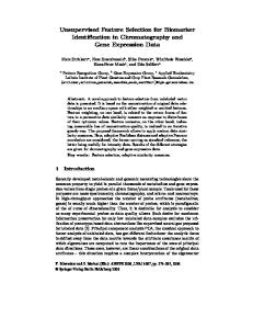
adaptive histograms. Fraser’s algorithm could be considered a middle step between kernel and histogram methods, because its accuracy is closer to the kernel’s, and it is as fast as histogram based methods. In this work an enhancement over the MIFS and MIFS-U methods is proposed, to overcome their limitations in highdimensional feature spaces. An adaptive selection criterion is proposed such that, the tradeoff between discarding redundancy or irrelevance is adaptively controlled, eliminating the need of an user defined parameter. Next section describes the procedure for estimating the MI. In section III the limitations of MIFS and MIFS-U methods are analyzed. In section IV the proposed feature selection method called AMIFS, is presented. In section V the artificial and benchmark datasets used in the simulations are described. Section VI shows the simulation results, as well as their discussion. Finally, section VII presents the conclusions. II. M UTUAL I NFORMATION E STIMATION To deal with data of mixture nature (discrete and continuous features) an extended version of Fraser’s algorithm is introduced for computing the MI for continuous features and discrete probabilities are used in the case of discrete features. A. Extended Fraser’s Algorithm One of the foundations of the Fraser’s algorithm [10] is the invariance of MI with respect to transformations acting on individual coordinates. Under this assumption, Fraser introduced a change of variable to simplify the counting operations. It consists in mapping each floating point feature sample into integers in the [0, N − 1] interval, preserving the original order of the elements in the transformed space. However, in practice although the nature of the feature may be continuous, it is uncommon to obtain a feature sampling without repeated elements. In many well-known benchmark datasets available at the UCI repository [11], the average percentage of repeated elements is rather high, for instance, this figure is 35% in the Noisy Waveform Dataset, 77% in the Iris Dataset, and 92% in the Vehicle Dataset. Assigning a different integer label to two or more repeated floating point values, may result in an incorrect MI estimation. Fig. 1 shows an example of mapping features onto the interval [0, N − 1], following an ascending order. In this example the value 0.5 is repeated twice in feature f2 . As a consequence, there are 2 possible label combinations for these elements, called a and b. Depending on the random choice of labels, these points could be assigned to distinct partitions in each case (Box1 and Box2 in Fig. 1), causing a different pdf estimation. The correct procedure is to assign the same label to equal floating point values. Therefore, in the stage of building histograms, we consider only Nr labels instead of N , with Nr < N , where Nr is the number of samples in the feature vector with different floating point values, and N is the dimension of the feature vector. To quantify the effect of repeated elements in the MI estimation by using Fraser’s original algorithm, the following test was made. A random variable was generated from a
uniform distribution with 1% of repeated elements (F1 ) and it was scaled into different intervals for obtaining a second variable with different percentage of repeated elements (F2 ). Table I shows that the greater the number of repeated values, the larger is the difference between the MI estimated with the original Fraser’s algorithm and the proposed modification. Therefore in high-dimensional feature spaces, the original Fraser’s algorithm could lead to wrong MI estimations and bad performances of the feature selection algorithms. Notice that the extended Fraser’s algorithm includes the original one, i.e. when there are no repeated elements the two algorithms are exactly the same. f1 0,2 0,5 0,1 0,3 0,8
f1 0,2 0,5 0,1 0,3 0,8
f2 0,5(a) 0,4 0,6 0,2 0,5(b)
f2 0,5(b) 0,4 0,6 0,2 0,5(a)
Discret1 −→
f1 1 3 0 2 4
Discret2 −→
f1 1 3 0 2 4
f2 2(a) 1 4 0 3(b)
f2 3(b) 1 4 0 2(a)
Sort1 (f1 (f2 )) −→
f1 0 1 2 3 4
Sort2 (f1 (f2 )) −→
f1 0 1 2 3 4
f2 4 2(a) Box1 0 1 Box2 3(b)
f2 4 3(b) Box1 0 1 Box2 2(a)
Fig. 1. Example showing that assigning different labels to equal floating point values, may lead to an incorrect MI estimation in Fraser’s original algorithm
TABLE I D IFFERENCES IN THE MI ESTIMATION BETWEEN THE ORIGINAL F RASER ’ S ALGORITHM AND THE PROPOSED MODIFICATION , DUE TO THE PRESENCE OF REPEATED VALUES WITHIN A FEATURE
% Repeated values F1 (1%) - F2 (20%) F1 (1%) - F2 (40%) F1 (1%) - F2 (50%) F1 (1%) - F2 (70%) F1 (1%) - F2 (80%) F1 (30%) - F2 (50%) F1 (40%) - F2 (70%)
MI (Fraser’s orig.) 5.549 5.478 5.515 5.330 5.322 5.511 5.434
MI (Fraser’s mod.) 5.058 4.979 4.960 4.663 4.590 4.932 4.663
III. L IMITATIONS OF MIFS AND MIFS-U IN 1 H IGH -D IMENSIONAL F EATURE S PACES The MIFS algorithm is as follows: 1) (Initialization) set F ← “initial set of n features” S ← “empty set”. 2) (Computation of the MI with the output class) ∀fi ∈ F compute I(C; fi ). 3) (Selection of the first feature) find the feature fi that maximizes I(C; fi ); set F ← F \{fi }; set S ← {fi }. 4) (Greedy selection) repeat until |S| = k. a) (Computation of the MI between variables) ∀fi ∈ F and ∀fs ∈ S compute I(fi ; fs ). b) (Selection of the next feature) choose the feature fi ∈ F that maximizes P I(C; fi ) − β s∈S I(fs ; fi ); set F ← F \{fi }; set S ← {fi }.
5) Output the set S containing the selected features. The MIFS-U algorithm only changes the selection criterion of MIFS, corresponding to step 4b, which is rewritten as: X I(C; fs ) I(fs ; fi ). (1) I(C; fi ) − β H(fs ) s∈S
In both algorithms the selection criterion is composed of two terms, see for instance (1). The left hand term measures the relevance of the feature to be added (information about the class) and the right hand term limits the score assigned to that feature, in order to avoid including a redundant feature in the selected feature set. The right hand term in both MIFS and MIFS-U is a cumulative sum that is subtracted to the first term, which estimates heuristically the redundancy among the selected features. Because this term is a cumulative sum, it grows in magnitude with respect to the first term, specially for high-dimensional feature spaces. When the left hand term becomes negligible with respect to the right hand term, the feature selection algorithm is forced to select non-redundant features with the already selected ones. This may cause the selection of irrelevant features earlier than the redundant ones. On the other side, both algorithms relies on the parameter β for controlling the redundancy penalization, whose optimal value is strongly dependent on the problem at hand. IV. A DAPTIVE MIFS Let’s analyze first the relation between redundancy and MI between two features. The I(fi , fs ) can take values in the following interval [12]: 0 < I(fi ; fs ) < M in{H(fi ), H(fs )}
(2)
where H(fi ) corresponds to the entropy of the feature fi . The Fig. 2 illustrates expression (2), in particular if one feature is completely redundant with the other then the MI is maximum. The proposed selection criterion for AMIFS is as follows: X I(fs ; fi ) (3) I(C; fi ) − e s∈S Ns H(f ) where, e ) = M in{H(fs ), H(fi )} H(f
(4)
and Ns is the number of already selected features. The right hand term in (3) is an adaptive redundancy penalization term, which corresponds to the average of the MI between each pair of selected features, divided by the minimum entropy between them. Comparing (3) with (1) or with the expression in step 4b. of the MIFS algorithm, it can be seen that the parameter β has been replaced by an adaptive term given by the denominator of the summation argument in (3). In MIFS-U, see (1), the redundancy penalization term always divide the I(fi ; fs ) by the entropy of the selected features H(fs ). If H(fs ) is greater than the entropy of the candidate feature H(fi ), the MIFS-U algorithm would give
more importance to the relevance, instead of penalizing the redundancy more strongly. In summary, AMIFS modifies the step 4b. as follows: 4) (Greedy selection) repeat until |S| = k. a) (Computation of the MI between variables) ∀fi ∈ F and ∀fs ∈ S compute I(fi ; fs ). b) (Selection of the next feature) choose theP feature fi ∈ F that maximizes I(fs ;fi ) ; set F ← F \{fi }; I(C; fi ) − s∈S N e s H(f ) set S ← {fi }. The entropy is calculated at the same stage than estimating the MI with the output class I(C; fs ). Therefore, AMIFS has about the same computational cost than MIFS, i.e. O(N logN ).
Fig. 2.
Relations between Entropy and MI
V. DATASETS A. Artificial Datasets Two artificial datasets were created to compare the performances of AMIFS, MIFS and MIFS-U when there are many irrelevant and redundant features. 1) Test 1 (Gaussian Multivariate Dataset): This dataset consists of two clusters of points generated from two different 10th-dimensional normal Gaussian distributions. Class 1 corresponds to points generated from N (0, 1) for each dimension and Class 2 to points generated from N (4, 1). For illustration purposes Fig. 3 shows a three-dimensional version of the problem. This dataset consists of 50 features and 500 samples per class. By construction, features 1-10 are equally relevant, features 11-20 are completely irrelevant and features 21-50 are highly redundant with the first ten features. Ideally, the order of selection should be first the relevant features 1-10, then the redundant features 21-50, and finally, the irrelevant features 11-20. 2) Test 2 (Uniform Hypercube Dataset): This dataset consists of two clusters of points generated from two different 10th-dimensional hypercube [0, 1]10 , with uniform distribution. The relevant feature vector (f1 , f2 , . . . , f10 ) was generated from this hypercube in decreasing order of relevance from feature 1 to 10. A parameter α = 0.5 was defined for the relevance of the first feature and a factor γ = 0.8 for decreasing the relevance of each feature. A pattern belongs to Class 1 if (fi < γ i−1 ∗ α / i = 1, . . . , 10), and to Class 2 otherwise. For illustration purposes Fig. 7 shows a three-dimensional version of the problem. As it can be seen, feature F1 is more discriminative than F2, and F2 is more discriminative than F3.
This dataset consists of 50 features and 500 samples per class. By construction, features 1-10 are relevant, features 11-20 are completely irrelevant, and features 21-50 are highly redundant with the first ten. Ideally, the order of selection should be first the relevant features 1-10 (with feature 1 in the first position and feature 10 in the last position), then the redundant features 21-50, and finally, the irrelevant features 11-20.
MIFS-U was set at the value recommended by the respective authors, β = 0.7 for MIFS and β = 1 for MIFS-U. TABLE II S UMMARY OF DATASETS U SED Name Noisy Waveforms Ionosphere Sonar
No features 40 34 60
No examples 1000 351 204
No classes 3 2 2
B. Benchmark Datasets The AMIFS algorithm was tested on three well-known data bases from the UCI repository [11]. In table II a summary of the datasets used is presented. A multilayer perceptron with a single hidden layer, trained by a Quasi-Newton second order learning method (BPQ) [13] was used as a classifier. All the simulation results presented in the next section, correspond to the average of 10 trials of 200 epochs each, with different random initializations. In a first stage the optimal number of hidden units for each problem was experimentally determined. With this aim, the datasets were divided into three subsets: 50% for training, 25% for validation and 25% for testing. The highest classification rate in the validation set was used to select the best architecture. The performances of AMIFS, MIFS and MIFS-U in the Ionosphere and Sonar datasets, were compared using the classification rates on the test set for different numbers of features selected. 1) Breiman’s Noisy Waveform Dataset: In this problem three 21-dimensional vectors or waveforms in R21 are given. The patterns in each class are defined as random convex combinations of two of these vectors (waves (1, 2); (1, 3); (2, 3) generate respectively classes C1 , C2 , C3 ). In the noisy version of the problem 19 additional noise components N (0, 1) are added to each pattern. The dataset has 1000 examples (33% per class). The ideal order of selection is first the relevant features 1-21 (all these features have the same relevance) and then the irrelevant features 22-40. 2) Ionosphere Dataset: In this case the goal is to identify the presence of some kind of structure in the ionosphere from the returns of radar signals. It is a two-class problem, where “Good” radar returns are those showing evidence of some type of structure and “Bad” returns are those that do not. The dataset has 351 patterns and 34 input features. The architecture of the neural net used was 34-5-2. 3) Sonar Dataset: The problem consists in discriminating between the sonar returns bounced off a metal cylinder and those bounced off a rock. It is a two-class problem: metal or rock. There are 60 input features per each instance. Because the number of examples is very small (208 patterns), a new partition of the dataset was made for comparing the selection algorithms. It was partitioned into 104 patterns for training and 104 for testing. The neural net architecture used in this problem was 60-5-2. In all methods the MI was calculated using the extended version of the Fraser’s algorithm for continuous features. In all the experiments the parameter of the algorithms MIFS and
VI. S IMULATION R ESULTS Figs. 4-6 show the simulation results obtained with the Gaussian Multivariate dataset for the MIFS, MIFS-U and AMIFS algorithms, respectively. The x-axis in these figures represents the order of selection, and the y-axis represents the feature selected at the corresponding ranking position. For instance, in Fig. 4 the feature selected at the 11th position is the number 20. Likewise, Figs. 8-10 show the simulation results obtained with the Uniform Hypercube dataset. In both artificial datasets, AMIFS selected the features following the ideal order, firstly the relevant features, secondly the redundant ones and finally the irrelevant ones. In contrast, MIFS and MIFS-U had a bad performance in these datasets, selecting some irrelevant or redundant features earlier than the relevant ones. In the Uniform Hypercube dataset, both MIFS and MIFS-U selected some irrelevant features earlier than redundant features, because they penalize too much the redundancy. Figs. 11-13 show the simulation results on the Breiman‘s Noisy Waveform dataset, for the MIFS, MIFS-U and AMIFS algorithms, respectively. In this dataset, AMIFS correctly selected 18 out of 21 relevant features, while MIFS-U selected 16 correct features and MIFS only 9 correct features. Table III shows the mean classification rates obtained in the test set for the Ionosphere dataset, using the three feature selection algorithms. In this dataset, AMIFS outperformed both MIFS and MIFS-U for different numbers of selected features. Table IV shows that the difference in mean classification rates between AMIFS and MIFS are statistically significant according to the t-student test for 3, 5, 9 and 15 selected features. Moreover, the difference in mean classification rates between AMIFS and MIFS-U are statistically significant according to the t-student test for 5 and 15 selected features. Table V shows the mean classification rates obtained in the test set for the sonar dataset, using the three feature selection algorithms. In this dataset, AMIFS outperformed both MIFS and MIFS-U for different numbers of selected features. Table VI shows that the difference in mean classification rates between AMIFS and MIFS are statistically significant according to the t-student test for 4, 7 and 15 selected features. Moreover, the difference in mean classification rates between AMIFS and MIFS-U are statistically significant according to the t-student test for 4, 7, 11 and 15 selected features.
0.9
6
0.8
5
0.7
4
0.6 F3
F3
1
7
3 2
0.5 0.4
1
0.3
0
0.2
8
−1 −2 2 6
2
−2
−4
0.4
0.6 0.4
−2
0
F2
0.6 0.8
F1
0
4
0.8
0 1
4 −3 8
Fig. 3.
1
0.1
6
Illustration of the Gaussian Multivariate dataset in three dimensions
Fig. 7.
F1
0.2
0.2
F2
0
−4
0
Illustration of the Uniform Hypercube dataset in three dimensions 50
50 45 45 40 40 35
feature number
feature number
35
30
25
30
25
20
20 15 15 10 10 5 5 0 0
0
5
10
15
20
25
30
35
40
45
0
5
10
15
20
25
30
35
40
45
50
selection order of features
50
selection order of features
Fig. 4. Ranking of Features in the Gaussian Multivariate dataset by using MIFS with β = 0.7
Fig. 8. Ranking of Features in the Uniform Hypercube dataset by using MIFS with β = 0.7 50
50 45 45 40 40 35
feature number
feature number
35
30
25
30
25
20
20 15 15 10 10 5 5 0 0
0
5
10
15
20
25
30
35
40
45
0
5
10
15
20
25
30
35
40
45
50
selection order of features
50
selection order of features
Fig. 5. Ranking of Features in the Gaussian Multivariate dataset by using MIFS-U with β = 1
Fig. 9. Ranking of Features in the Uniform Hypercube dataset by using MIFS-U with β = 1 50
50
45
45
40
40
35
feature number
feature number
35
30
25
20
25
20
15
15
10
10
5
5
0
30
0
0
5
10
15
20
25
30
35
40
45
50
selection order of features 0
5
10
15
20
25
30
35
40
45
50
selection order of features
Fig. 6. Ranking of Features in the Gaussian Multivariate dataset by using AMIFS TABLE III C LASSIFICATION R ATES IN T EST S ET (I ONOSPHERE DATASET ) No of features 3 5 9 15 All (34)
AMIFS 90.23 90.34 91.38 90.46
MIFS 83.10 85.52 84.83 88.05 91.95
MIFS-U 89.54 85.86 91.26 88.62
Fig. 10. AMIFS
Ranking of Features in the Uniform Hypercube dataset by using TABLE IV
R ESULTS OF T- STUDENT TEST FOR M EAN C LASSIFICATION R ATES IN THE I ONOSPHERE DATASET No of features 3 5 9 15
p-value AMIFS/MIFS 6.68e-05 5.9e-09 1.3e-04 0.003
p-value AMIFS/MIFS-U 0.715 4.39e-08 0.909 0.011
40
VII. C ONCLUSIONS
35
feature number
30
25
20
15
10
5
0
0
5
10
15
20
25
30
35
40
selection order of features
Fig. 11. Ranking of Features in the Breiman‘s Noisy Waveform dataset by using MIFS with β = 0.7 40
35
feature number
30
25
20
15
10
The proposed AMIFS method of feature selection is an enhancement over the MIFS and MIFS-U algorithms that are based on mutual information. The previous methods present limitations when there are many redundant and irrelevant features, because they overweight the redundancy penalization term in the selection criterion. AMIFS overcomes this limitation by adjusting adaptively the trade-off between eliminating irrelevance or redundancy, and getting rid of the need of an user defined parameter. The AMIFS method can be applied to data of mixed nature (discrete and continuous features). An extended version of Fraser‘s algorithm was used to estimate the mutual information among continuous variables that may have repeated floating point values. AMIFS is as fast and computationally efficient as MIFS, O(N logN ), with a slight extra burden to calculate entropies. The AMIFS method surpassed MIFS and MIFS-U in two artificial datasets and three benchmark problems. ACKNOWLEDGMENT
5
0
0
5
10
15
20
25
30
35
40
selection order of features
Fig. 12. Ranking of Features in the Breiman‘s Noisy Waveform dataset by using MIFS-U with β = 1
R EFERENCES
40
35
feature number
30
25
20
15
10
5
0
The authors would like to thank Pedro Ortega for his help in implementing the MIFS algorithm and his useful and fruitful comments about this work. This research was supported in part by Conicyt-Chile under grant Fondecyt 1030924.
0
5
10
15
20
25
30
35
40
selection order of features
Fig. 13. Ranking of Features in the Breiman‘s Noisy Waveform dataset by using AMIFS TABLE V C LASSIFICATION R ATES IN T EST S ET (S ONAR DATASET ) No of features 4 7 11 15 All (60)
AMIFS 80.19 85.19 84.04 86.73
MIFS 78.17 83.46 83.85 85.19 80.67
MIFS-U 76.25 76.92 76.35 82.98
TABLE VI R ESULTS OF T- STUDENT TEST FOR M EAN C LASSIFICATION R ATES IN THE S ONAR DATASET No of features 4 7 11 15
p-value AMIFS/MIFS 9.08e-05 2.81e-07 0.443 0.013
p-value AMIFS/MIFS-U 2.84e-08 1.61e-12 1.86e-10 2.79e-06
[1] A. K. Jain, R. P. W. Duin, and J. Mao, ”Statistical Pattern Recognition: A Review”, IEEE Trans. on Pattern Analysis and Machine Intelligence, vol. 22, no. 1, pp. 4-37, Jan. 2000. [2] J. Kohavi, K. Pfleger, ”Irrelevant Features and the Subset Selection Problem”, in Proc. 11th Int. Conference on Machine Learning, 1994, pp. 121-129. [3] K. Kira, L. A. Rendell, ”The Feature Selection Problem: Traditional methods and a new algorithm”, in Proc. 9th Int. Conference on Machine Learning, pp. 129-134, 1992. [4] M. Modrzejewski, ”Feature Selection Using Rough Sets Theory”, in Proc. European Conference on Machine Learning, pp. 213-226, 1993. [5] H. Almuallim, T. G. Dietterich, ”Learning With Many Irrelevant Features”, in Proc. 9th National Conference on Artificial Intelligence, MIT Press, pp. 547-552, 1992. [6] R. Battiti, ”Using Mutual Information for Selecting Features in Supervised Neural Net Learning”, IEEE Trans. on Neural Networks, vol. 5, no. 4, pp. 537-550, July 1994. [7] N. Kwak, C.-H. Choi, ”Input Feature Selection for Classification Problems”, IEEE Trans. on Neural Networks, vol. 3, no. 1, pp. 143-159, 2002. [8] N. Kwak, C.-H. Choi, ”Input Feature Selection by Mutual Information Based on Parzen Windows”, IEEE Trans. on Pattern Analysis and Machine Intelligence, vol. 24, no. 12, pp. 1667-1671, Dec. 2002. [9] K. Torkkola, ”Feature Extraction by Non-Parametric Mutual Information Maximization”, Journal of Machine Learning Research, vol. 3, pp. 14151438, 2003. [10] A. M. Fraser, H. L. Swinney, ”Independent Coordinates for Strange Attractors from Mutual Information”, Physical Review A, vol. 33, no. 2, pp. 1134-1140, 1986. [11] C. L. Blake, C. J. Merz, UCI Repository of Machine Learning Databases, (http://www.ics.uci.edu/ mlearn/MLRepository.html), 1998. [12] T. M. Cover, J. A. Thomas, Elements of Information Theory, John Wiley & Sons, New York, 1991. [13] K. Saito, R. Nakano, ”Partial BFGS Update and Efficient Step-Length Calculation for Three-Layer Neural Networks”, Neural Computation 9, pp. 123-141, 1997.