Reconsidering Mutual Information Based Feature Selection: A Statistical Significance View Nguyen Xuan Vinh

Jeffrey Chan

James Bailey

Department of Computing and Information Systems The University of Melbourne, VIC 3010, Australia

Abstract Mutual information (MI) based approaches are a popular feature selection paradigm. Although the stated goal of MI-based feature selection is to identify a subset of features that share the highest mutual information with the class variable, most current MI-based techniques are greedy methods that make use of low dimensional MI quantities. The reason for using low dimensional approximation has been mostly attributed to the difficulty associated with estimating the high dimensional MI from limited samples. In this paper, we argue a different viewpoint that, given a very large amount of data, the high dimensional MI objective is still problematic to be employed as a meaningful optimization criterion, due to its overfitting nature: the MI almost always increases as more features are added, thus leading to a trivial solution which includes all features. We propose a novel approach to the MI-based feature selection problem, in which the overfitting phenomenon is controlled rigourously by means of a statistical test. We develop local and global optimization algorithms for this new feature selection model, and demonstrate its effectiveness in the applications of explaining variables and objects.

Introduction Within the rich literature on feature selection, mutual information (MI) based approaches form an important paradigm. Over years, these methods have gained large popularity, thanks to their simplicity, effectiveness and strong theoretical foundation. Given an input data of M features X = {X1 , . . . , XM }, and a target classification variable C, the goal of MI-based feature selection is to select the optimal e1 , . . . , X em } that shares the maximal e ∗ = {X feature subset X mutual information with C, defined as ! X e C) P (X, e e I(X; C) , P (X, C) log (1) e (C) P (X)P e X,C

Despite its theoretical merit, implementing this so-called Max-Dependency criterion is challenging, due to the difficulties in estimating the multivariate probability distrie and P (X, e C) from limited samples. Therebutions P (X) c 2014, Association for the Advancement of Artificial Copyright Intelligence (www.aaai.org). All rights reserved.

fore, all current MI-based methods approximate this MaxDependency criterion with low dimensional MI quantities, in particular the relevancy I(Xi ; C), joint relevancy I(Xi Xj ; C), conditional relevancy I(Xi ; C|Xj ), redundancy I(Xi ; Xj ) and conditional redundancy I(Xi ; Xj |C). These low-dimensional MI quantities capture only loworder feature dependancy. Seventeen low-dimensional MIbased criteria can be found in (Brown et al. 2012), summarizing two decades of research in this area. The reason for abandoning the Max-Dependency criterion in Eq. (1), is commonly attributed to the technical difficulties encountered in estimating the joint multivariate densie and P (X, e C) with limited samples (Peng, Long, ties P (X) and Ding 2005). In our opinion, besides this practical constraint, there exists a more fundamental theoretical limitation with using the Max-Dependency criterion, that has to do with the monotonicity property of the mutual information: the MI never decreases when including additional variables, e ∪ Xi ; C) ≥ I(X; e C) (Cover and Thomas 2006; that is, I(X de Campos 2006). Thus, adding more features into the set e will likely increase the value of the Max-Dependency X e ≡ 0, which rarely occurs in criterion, unless I(Xi ; C|X) practice, due to statistical variation and chance agreement between variables. The Max-Dependency criterion is therefore usually maximized when all variables in X are included. Due to this overfitting nature of the mutual information measure, the Max-Dependency criterion cannot be employed as a meaningful optimization criterion for feature selection, even when large samples are available. Contribution: We take a novel view of the MI-based feature selection problem that is based on the high-dimensional Max-Dependancy criterion in (1). We propose to systematically and rigourously resolve the overfitting issue by means of using a statistical test of significance for the MI. We formulate novel local and global optimization criteria, and propose effective solutions for these problems. Finally, we demonstrate the usefulness of our proposed approaches in the applications of explaining variables and objects in data.

A new framework for incremental high dimensional MI-based feature selection Let us begin by considering the Max-Dependency criterion in Eq. (1) and proposing an incremental optimization proce-

dure similar to other popular MI-based heuristics. Suppose e m−1 and would we have already selected the feature set X em . e like to expand it to Xm by adding an additional feature X Due to the decomposition property of the mutual information (Cover and Thomas 2006) em ; C|X e m ; C) = I(X e m−1 ; C) + I(X e m−1 ) I(X

(2)

em is thus the conthe incremental objective value added by X e e m−1 ). Since ditional mutual information (CMI) I(Xm ; C|X the CMI is non negative, adding any arbitrary feature to e m−1 will almost surely increase the Max-Dependency criX terion, due to chance agreement. To rectify the overfitting nature of the Max-Dependency criterion, we propose to proceed as follows. While the Max-Dependency criterion will always increase, the magnitude of this increment becomes e m , i.e., smaller and smaller as more features are added to X adding an additional feature improves little knowledge about C. Indeed we can expect that at some point, this increment will be so small that it becomes statistically insignificant. Information theory provides us with an important tool to quantify the statistical significance of this increment. We consider the following classical result by Kullback (Kullback 1968; de Campos 2006), which, in the specific context of feature selection, can be stated as follows: em and C are Theorem 1. Under the null hypothesis that X e conditionally independent given Xm−1 , the statistic em ; C|X em , X e m−1 ) approximates to a χ2 (l(X e m−1 )) 2N ·I(X e e distribution, with l(Xm , Xm−1 ) = (rC − 1)(e rm − 1)re Xm−1

degree of freedom, where rem , rC and rXem−1 are the number em , C and X e m−1 respectively, and N is the of categories of X number of samples. Herein, we assume that all features have been discretized e to categorical variables. Note that in case X = ∅, then Qm−1 m−1 rXem−1 = 1. Otherwise rXem−1 = i=1 rei , where rei is the ei . In general, the theorem also number of categories of X em and C are, each of them, a holds for the case where X set of random variables (RV), rather than a single RV. In such case, rXem and rC shall be the aggregate number of categories of such a RV set, similar to rXem−1 . We note that the quantity 2N.I(X1 ; X2 ) is in fact the well known Gstatistic for the test of independence between random variables. Kullback’s statistic is more general, in that it also provides a means for testing conditional independence. This result provides us with a rigorous means to control the overfitting problem. Only features that are statistically significantly dependent on the class variable C, given all the other already selected features, should be included. Given a statistical significance threshold α, we propose an incremental feature selection scheme for maximizing the MaxDependancy criterion (1) as in Algorithm 1. Here, χα,l(Xem ,Xem−1 ) is the critical value corresponding to a given significance level 1 − α, i.e. the value such that the em , X e m−1 )) ≤ χ probability Pr(χ2 (l(X em ,X e m−1 ) ) equals α,l(X e e α, where the degree of freedom l(Xm , Xm−1 ) is determined

Algorithm 1 iSelect : incremental Feature Selection e m−1 , a new feature: Repeat given X em = arg max I(Xi ; C|X e m−1 ) − 1 χ X e 2N α,l(Xi ,Xm−1 ) e Xi ∈X\Xm−1 em ; C|X e m−1 ) > 1 χ can be added, if I(X e m ,X e m−1 ) . 2N α,l(X Until no more feature could be added.

as per Theorem 1. If we take α = 0.95, then the MI test of independence is at the traditional threshold of 5% significance. If we take α = 0.99, then the MI test of independence is at the strict threshold of 1% significance. With this selection scheme, we add the feature that has the most statistically significant conditional MI with the class variable C, given all the previously added features, until no more feature can be added. A reasonable starting set is the single feature that has the maximum (unconditioned) MI with C, or the set of two features that jointly shares the maximum MI with C. The significance threshold α serves to control the model complexity, i.e. number of features to be included. The lower the α value, the more relaxed the statistical test, and thus more features will be selected. The computational complexity of adding the m-th feature is O((M − m)mN ).

High dimensional MI-based feature selection as a global optimization problem In the previous section, we discussed an incremental, greedy scheme for MI-based feature selection. Similar to other MIbased greedy approaches, this heuristics will only converge to a locally optimal solution at best. We next formalize the feature selection problem as a global optimization problem, maximizing the adjusted dependancy defined as: 1 χ e (3) 2N α,l(X,∅) Qe e ∅) = ( |X| Here, the degree of freedom l(X, ei −1)(rC −1) i=1 r is determined as per Theorem 1. The intuition behind this objective is clear: we aim to find the feature set with the best mutual information with the class variable, but penalizing it according to the significance of the MI value. Larger feature sets always yield higher mutual information, but not necessarily better adjusted dependancy overall. An appealing interpretation for the Max-Adjusted Dependancy criterion in (3) is in terms of model goodness-of-fit and model come C) measures model goodness-of-fit—the more plexity. I(X; variables we add, the more information they carry about C. The price to pay is, however, an increment in model com1 χα,l(X,∅) plexity, as measured by 2N e , which increases as the feature set grows. e ∗ of X that The optimization task is to find the subset X e C) globally maximizes the adjusted dependency score D(X; in Eq. (3). The na¨ıve exhaustive enumeration search is presented in Algorithm 2. It systematically enumerates feature sets of increasing size m. This is clearly not a viable option, requiring exponential time, as there are 2M − 1 subsets. In e C) , D(X;

e C) − I(X;

e , p(X)

1 χ e . 2N α,l(X,∅)

2 goodness−of−fit g*(m) complexity penalty p(m) D*(m) I(X;C)

1.5

1

p(m), g*(m)

the next section, we will show how the globally optimal solution can be identified in polynomial time instead. The key insight into this development is that, we can bound the maximum feature set cardinality, above which any feature set of higher cardinality cannot be optimal. For ease of exposition, we shall start by considering the simpler case where all features have the same number of categories, and then later relax this assumption. We first define the penalty function as

0.5

0

−0.5 me −1

0

2

4 6 Number of features m

Algorithm 2 Na¨ıve global search e ∗ := ∅ X for m = 1 to M do e ∗m := arg maxe {D(X e m ; C)|X e m ⊂ X; |X e m | = m} X Xm ∗ ∗ ∗ ∗ e e e e If D(Xm ; C) > D(X ; C) then X := Xm . end for

m* 8

10

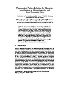
Figure 1: The relationship between the adjusted dependancy, goodness of fit and penalty Theorem 2. (Max-Cardinality) The size of the optimal feae ∗ | is not greater than m∗ , max{m| p(m) < ture set |X I(X; C)} .

All features have the same number of categories The following properties will be algorithmically important: Property 1. For all feature sets of the same size, the penalty terms p(·) are the same. e we can write p(|X|), e or Thus, instead of writing p(X), p(m), with the implication that any arbitrary feature set e = m gets this same penalty of p(m) = of size |X| 1 m χ 2N α,(rC −1)(k −1) . Property 2. p(m), m ∈ Z+ is a non-negative, monotonic non-decreasing function in m. This holds true, based on the fact that for a fixed significance level α, the critical threshold χα,l of the Chi-squared distribution increases as the degree of freedom l increases (Myers and Well 2003). We now define

Proof. Clearly when p(m) has grown larger than the maximum goodness of fit I(X; C), then the best adjusted dependancy score D∗ (m) for any m > m∗ will be < 0, and thus can not be globally optimal, noting that we have D(∅; C) = 0. Thus, in the worst case, we only need to search among feature sets of cardinality ≤ m∗ , which is characterized by the following result. Theorem 3. m∗ ≤ dlogk ( 2N.I(X;C) + 1)e − 1 rC −1 Proof. If we can identify the minimum integer m b satisfying

as the best goodness of fit of all feature sets of size m. Property 3. g ∗ (m) is a monotonic non-decreasing function upper-bounded by I(X; C).

1 χ ≥ I(X; C) m c 2N α,(rC −1)(k −1) then m∗ ≤ m b − 1. Unfortunately, since m b does not admit a closed-form solution, as χα,l does not have an analytical form, we provide an over-estimate for m b as follows. Note that χα,l is the value such that p(χ2 (l) ≤ χα,l ) = α. Since generally we use α  0.5, the mean value l of the χ2 (l) distribution is an under-estimate for χα,l , i.e.,

Let us also define D∗ (m) , g ∗ (m) − p(m), i.e., the best adjusted dependancy score of all feature sets of size m, then clearly e C) = max D∗ (m) max D(X; (5)

1 1 b χα,(rC −1)(km (rC − 1)(k m − 1) c −1)  2N 2N Now we will require a stricter condition for m, b that is

g ∗ (m) ,

max

e C) I(X;

(4)

e e X⊂X,| X|=m

m∈[1,M ]

The relationship between these quantities is illustrated in Figure 1. The best goodness of fit g ∗ (m) is monotonically non-decreasing in m, and approaches its upperbound I(X; C) as m increases. The penalty term p(m) grows strictly monotonically increasing in m. The best adjusted dependancy score D∗ (m) is the difference between g ∗ (m) and p(m). It can be observed that once the complexity penalty p(m) is larger than the maximum goodness of fit I(X; C), then D∗ (m) becomes negative and will remain so as m increases. This observation suggests us that an exhaustive search on all m values is not necessary.

p(m) b ≥ I(X; C) ⇔

1 b (rC − 1)(k m − 1) 2N ⇔m b

≥ I(X; C) ≥ logk (

2N.I(X, C) + 1) (6) rC − 1

For m ≥ logk ( 2N.I(X,C) + 1), we have p(m) ≥ I(X; C), rC −1 thus m∗ ≤ dlogk ( 2N.I(X;C) + 1)e − 1. rC −1 Let m b ∗ , dlogk ( 2N.I(X;C) + 1)e − 1, then the largest set rC −1 size we have to search is m b ∗ . In fact, we may even terminate the search before m reaches m b ∗.

Theorem 4. (Early stop) Suppose the search is currently at e ∗ . If I(X; C) − I(X e ∗ ; C) ≤ m = me , the current best set is X p(me + 1) − p(me ), then the globally optimal feature set e∗. size is X

threshold χα,l of the Chi-squared distribution increases as the degree of freedom l increases (MyersQand Well 2003). m Herein it is easily seen that (rC − 1)( i=1 ri+ − 1) ≤ Qm + e m , ∅) ≤ l(X e m , ∅). (rC − 1)( rei − 1), i.e., l(X

Proof. We are to decide whether to expand the feature set size to m ≥ me + 1. The maximum bonus for such exe ∗ ; C), while the addipansion is bounded by I(X; C) − I(X tional penalty is at least p(me + 1) − p(me ). If I(X; C) − e ∗ ; C) ≤ p(me + 1) − p(me ) then the adjusted depenI(X dancy score will always decrease as more features are added, e ∗ is the globally thus the search can be stopped at me and X optimal feature set.

Note that p∗ (m) is a non-negative, increasing function of m. It is straightforward to show that Theorem 4 still holds when p∗ (m) is used in place of p(m). Furthermore, Theorems 3 and 5 also hold true, where k is replaced by kmin , the smallest number of categories of features in X. Thus we can employ Algorithm 3 for this case, with k and p(m) replaced by kmin and p∗ (m). To further speed up the search, it is noted that for an m value, it is not needed to do a full exhaustive search on all feature sets of size m, thanks to the following observation: e Theorem 7. (Feature set bypassing) For any feature set X, ∗ ∗ e e e e if I(X; C) − I(X ; C) ≤ p(X) − p(X ), then X cannot be globally optimal and thus can be bypassed.

Using the results in Theorem 3 and 4, our proposed global approach, named GlobalFS, is presented in Algorithm 3. Algorithm 3 GlobalFS : Global Feature Selection e ∗ := ∅ X for m = 1 to dlogk ( 2N.I(X;C) + 1)e − 1 do rC −1 ∗ e e e m ⊂ X; |X e m | = m} Xm := arg maxe {D(Xm ; C)|X Xm

e ∗m ; C) > D(X e ∗ ; C) then X e ∗ := X e ∗m ; If D(X ∗ e ; C) ≤ p(m + 1) − p(m) then If I(X; C) − I(X ∗ e ; Exit;} {Return X end for

Theorem 5. GlobalFS admits a worst-case time complexity of O(M logk N N logk N ) in the number of features M , samples N and categories k. Proof. Clearly, the largest set size we have to consider is m b ∗ = dlogk ( 2N.I(X;C) + 1)e − 1. Assuming N  log rC ≥ rC −1 H(C) ≥ I(X; C), we have that m b ∗ ∼ logk N . As there m b∗ are O(M ) subsets of size up to m b ∗ and each set requires ∗ O(m b N ) time to process, the algorithm admits an overall complexity of O(M logk N N logk N ).

Features with different number of categories In this case, the penalty terms for feature sets of the same cardinality are no longer the same. Therefore, we shall replace the penalty function p(m) with p∗ (m) , e m ), that is, the minimum penalty minXem ⊂X,|Xem |=m p(X amongst all feature sets of size m, identified via the following result. Theorem 6. The minimum penalty p∗ (m) over all feature sets of size m corresponds to the set comprising m features of X with fewest number of categories. e+ X m

e +, . . . , X e + } be the set of m feaProof. Let = {X m 1 tures in X with the smallest number of categories, and e1 , . . . , X em } be m arbitrary features in X, with e m = {X X + the corresponding number of categories being {r1+ , . . . , rm } + e e and {e r1 , . . . , rem }. We show that p(Xm ) ≤ p(Xm ), i.e., χα,l(Xe+ ,∅) ≤ χα,l(Xem ,∅) . Indeed, this holds true, based on m the fact that for a fixed significance level α, the critical

i=1

∗

e represents the currently best soluProof. Recall that X e ∗ to any other set X, e the maximum tion. Moving from X bonus gained for the adjusted dependancy score is I(X; C)− e ∗ ; C), while the actual additional penalty incurred is I(X e − p(X e ∗ ). If the maximum bonus is smaller than the p(X) e cannot improve the current objecincurred penalty, then X tive value, and thus can be bypassed. The computational value of this theorem is that, for any feature set of size m, it takes O(mN ) time to process, which is mainly the time required for computing the mutual infore C). The penalty function, on the other hand, mation I(X; can be computed in O(1) time via a lookup table. Thus, using this simple check which costs O(1) time, a large amount of computation can be avoided. In Table 1, we recommend the best application scenario for each algorithm. iSelect and GlobalFS are both based on high-dimensional mutual information, and thus are most suitable for applications where a relatively large number of samples are available, e.g., from hundreds of samples. Due to its higher complexity, GlobalFS is suitable for problems with a small to medium number of features, e.g., several tens, whilst iSelect is recommended for problems having a larger number of features. Table 1: Algorithm summary #Samples N 10s 100s-1000s

#Features M 10s 100s-1000s Not applicable GlobalFS iSelect

Experimental evaluation We experimentally demonstrate the usefulness of the proposes approaches in two applications: Variable explanation and object explanation. Variable explanation aims to select a small set of variables that could potentially shed light

Table 2: Dataset summary. M: #features, N: #samples, #C: #classes Data Mushroom Waveform Dermatology Promoter Spambase Splice Optdigits Arrhythmia Madelon Multi-features Advertisements Gisette

M 21 21 34 57 57 60 64 257 500 649 1558 5000

N 8124 5000 366 106 4601 3190 3823 430 2000 2000 3279 6000

#C 2 3 6 2 2 3 10 2 2 10 2 2

Algorithm GlobalFS GlobalFS GlobalFS GlobalFS GlobalFS GlobalFS GlobalFS iSelect iSelect iSelect iSelect iSelect

on to the data generating process, i.e., explaining a target variable, often taken to be the class C. Object explanation, on the other hand, is a relatively novel problem, in which one aims to select a small set of features that distinguish the selected object from the rest of the data (Micenkova et al. 2013). Object explanation is often employed to explain outliers, but could be also used to explain any ordinary objects in principle. We compare our approach with other well-known MI based methods, namely maximum relevance (MaxRel), mutual information quotient (MIQ) (Ding and Peng 2003), conditional infomax feature extraction (CIFE) (Lin and Tang 2006), conditional mutual info maximization (CMIM) (Fleuret and Guyon 2004), joint mutual information (JMI) (Brown et al. 2012) and quadratic programming feature selection (QPFS) (Rodriguez-Lujan et al. 2010). Our implementation (in C++/Matlab–available from https://sites.google.com/site/vinhnguyenx) supports multithreading to maximally exploit the currently popular off-theshelf multicore architectures. A quad-core i7 desktop with 16Gb of main memory was used for our experiments, in which GlobalFS was executed with 6 threads running in parallel. We note that other incremental MI-based feature selection approaches, including iSelect, are generally fast even without parallelization.

Variable Explanation We employ several popular data sets from the UCI machine learning repository (Frank and Asuncion 2010) with varying dimensions and number data points, as summarized in Table 2. The aim of variable explanation is to select a relatively small set of features that are helpful in interpreting a target variable. Ideally, the ground-truth for evaluating this task would be, for each data set, a set of annotations indicating which features are important and which are not. Since this information is generally not available for real data, we thus employ the classification error rate as an indicative measure. For classifier, following (Herman et al. 2013; Rodriguez-Lujan et al. 2010) we employ support vector machine (Chang and Lin 2011) with linear kernel and the regularization factor set to 1. For MI computation, continuous features are discretized to 5 equal-frequency bins, while classification is performed on the original feature space. We

tested our algorithms with significance parameter at α = 0.99 and α = 0.95, corresponding to statistical tests at 1% and 5% significance respectively, but since the results are very similar, herein we report the results with α = 0.99. GlobalFS was tested on data sets with small to medium number of features. For larger dataset, we employed iSelect which is initialized using the two features with best adjusted dependancy score provided by GlobalFS. Note that both GlobalFS and iSelect automatically select the number of features, while other MI-based methods all require the number of feature as an input parameter. We use the number of features returned by GlobalFS/iSelect as input to these algorithms. The results of this experiment are detailed in Table 3, where we report the average error rate across 100 bootstrap runs. In each run, N bootstrap samples are drawn for the training set, while the unselected samples serve as the test set. In order to summarize the statistical significance of the findings, as in Herman et al., we employ the one sided paired t-test at 5% significance level to test the hypothesis that GlobalFS/iSelect or a compared method performs significantly better than the other. Overall we found that GlobalFS/iSelect perform strongly, consistently returning a small set of features that achieve high classification accuracy amongst the compared methods.

Object Explanation The object explanation task is to select a small set of features that distinguish the query object q from the rest of the data objects {o1 , . . . , on }. The task can be cast as a twoclass feature selection problem as proposed in (Micenkova et al. 2013), where the positive class is formed from n − 1 synthetic samples randomly picked from a Gaussian distribution centered at q, and the negative class is {o1 , . . . , on }. For this experiments, we employ a collection of data sets published by (Keller, Muller, and Bohm 2012) for benchmarking subspace outlier detection. The collection contains data sets of 10, 20, 30, 40, 50, 75 and 100 dimensions, each consisting of 1000 data points and 19 to 136 outliers. These outliers are challenging to detect, as they are only observed in subspaces of 2 to 5 dimensions and not in any lower dimensional subspaces. Our task here is not outlier detection, but to explain why the annotated outliers are designated as such, i.e., pointing out the subspace (feature set) in which the query point is outlying. For each outlier (query point) q, we form the positive class as proposed in (Micenkova et al. 2013), with samples drawn from N (q, λ2 I), where 1 λ = 0.35 · M · k-distance(q) and k-distance(q) is the distance from q to its k-th nearest neighbor, with k set to 35. The features are discretized to 5 equal-frequency bins, and mutual information based feature selection methods are employed to select the best features that distinguish the positive class from the negative class. Since the number of dimensions is moderate, we employ GlobalFS for this experiment. Again, we set our significance parameter at α = 0.99 and α = 0.95. GlobalFS automatically determines the number of features. We used the number of features of GlobalFS (α = 0.99) as the number of features to be selected by other MI-based methods. The ground-truth for this task is the outlying subspace for each outlier, available as part

Table 3: Bootstrap error rate comparison of GlobalFS/iSelect against other methods. W: win (+), T: tie (=), L: loss (−) for GlobalFS/iSelect against the compared method according to the 1-sided paired t-test. MIQ

CMIM

CIFE

MRMR

JMI

QPFS

0.6 ± 0.1 (=) 18.1 ± 5.5 (+) 28.0 ± 1.1 (+) 32.6 ± 0.8 (+) 23.5 ± 1.0 (=) 41.1 ± 4.4 (+) 18.9 ± 22.3 (−) 43.7 ± 2.8 (+) 5.6 ± 0.5 (−) 35.0 ± 2.3 (=) 38.4 ± 1.5 (+) 16.2 ± 0.6 (+) 7/3/2

1.4 ± 0.2 (+) 18.1 ± 5.5 (+) 26.1 ± 0.9 (=) 25.5 ± 0.8 (+) 38.6 ± 1.0 (+) 47.9 ± 4.8 (+) 21.9 ± 25.8 (+) 43.2 ± 2.9 (+) 8.1 ± 0.6 (+) 49.6 ± 2.0 (+) 37.9 ± 1.4 (−) 15.7 ± 0.6 (+) 10/1/1

0.6 ± 0.1 (=) 15.1 ± 4.7 (=) 26.0 ± 1.0 (=) 25.5 ± 0.8 (+) 23.5 ± 1.0 (=) 38.6 ± 3.8 (=) 18.9 ± 22.3 (−) 35.8 ± 3.0 (−) 6.6 ± 0.6 (=) 35.0 ± 2.3 (=) 38.6 ± 1.5 (+) 14.1 ± 0.6 (+) 3/7/2

0.6 ± 0.1 (=) 15.1 ± 4.7 (=) 26.0 ± 1.0 (=) 24.6 ± 0.8 (=) 29.9 ± 1.0 (+) 38.6 ± 3.8 (=) 18.9 ± 22.3 (−) 35.5 ± 2.9 (−) 6.6 ± 0.6 (=) 22.0 ± 1.2 (−) 38.4 ± 1.5 (+) 12.8 ± 0.8 (+) 3/6/3

1.4 ± 0.2 (+) 18.1 ± 5.5 (+) 26.0 ± 1.0 (=) 25.5 ± 0.8 (+) 23.5 ± 1.0 (=) 39.1 ± 3.8 (+) 20.3 ± 24.0 (+) 34.0 ± 3.0 (−) 6.6 ± 0.6 (=) 35.0 ± 2.3 (=) 38.0 ± 1.5 (−) 12.8 ± 0.6 (+) 6/4/2

0.6 ± 0.1 (=) 15.1 ± 4.7 (=) 26.0 ± 1.0 (=) 24.9 ± 0.8 (+) 23.5 ± 1.0 (=) 38.6 ± 3.8 (=) 18.9 ± 22.3 (−) 35.9 ± 2.9 (−) 5.6 ± 0.5 (−) 35.0 ± 2.3 (=) 38.3 ± 1.4 (+) 12.8 ± 0.8 (+) 3/6/3

1.5 ± 0.2 (+) 18.1 ± 5.5 (+) 28.0 ± 1.1 (+) 33.0 ± 0.9 (+) 27.5 ± 0.9 (+) 51.6 ± 3.4 (+) 25.3 ± 29.9 (+) 30.2 ± 2.9 (−) 7.8 ± 0.6 (+) 43.5 ± 1.8 (+) 38.4 ± 1.5 (+) 14.7 ± 1.1 (+) 11/0/1

GlobalFS α=0.99 GlobalFS α=0.95 MaxRel MIQ CMIM CIFE MRMR JMI QPFS

0.8 0.7 0.6 0.5

GlobalFS α=0.99 GlobalFS α=0.95 MaxRel MIQ CMIM CIFE MRMR JMI QPFS

0.9 0.8 0.7 0.6 Precision

Jaccard index

maxRel

0.4

3

10

2

10

1

10

0.5 0.4

0.3

0

10

−1

10

0.3

−2

0.2 0.1 0 10

GlobalFS/ iSelect 0.6 ± 0.1 15.1 ± 5.5 26.0 ± 1.1 24.6 ± 0.8 23.5 ± 1.0 38.6 ± 4.4 19.8 ± 22.3 38.4 ± 2.8 6.6 ± 0.5 35.0 ± 2.3 38.2 ± 1.5 11.7 ± 0.6

Naive Exhaustive Search GlobalFS α=0.99 GlobalFS α=0.95 MaxRel MIQ CMIM CIFE MRMR JMI QPFS

4

10

Time (s)

Data (#selected features) Mushroom(2) Promoter(2) Splice(2) Waveform(3) Spambase(3) Dermatology(2) Optdigits(3) Arrhythmia(3) Advertisements(3) Multi-features(3) Madelon(4) Gisette(2) #W/T/L:

20

30

40 50 60 70 Number of dimensions

80

(a) Average Jaccard index

90

100

0.2

10

0.1

10

0 10

−3

−4

20

30

40 50 60 70 Number of dimensions

(b) Average Precision

80

90

100

10

10

20

30

40

50 60 70 Number of dimensions

80

90

100

(c) Average execution time, Number of data points is ∼ 2000.

Figure 2: Evaluation of GlobalFS and other MI-based approaches on the object explanation task (best viewed in color). of Keller, Muller, and Bohm’s data. Let the true outlying subspace be T and the retrieved subspace be P , to evaluate the effectiveness of the algorithms, we employ the Jaccard index Jaccard (T, P ) , |T ∩ P |/|T ∪ P |, and the precision, precision , |T ∩ P |/|P |. The average Jaccard index and precision over all outliers for each dataset are reported in Figure 2(a,b). In this task, GlobalFS outperforms all the compared methods in both performance indices by a large margin. More specifically, for each number of dimensions M , we employ the one sided paired t-test at 5% significance level to test the hypothesis that GlobalFS or a compared method performs significantly better than the other. It turns out that across all M values, GlobalFS at both α = 0.95 and α = 0.99 significantly outperform all other approaches in both Jaccard index and precision. Although there is a slight difference in GlobalFS at different α values, this difference is found to be statistically insignificant, according to the t-test. An important factor that contributes to the strong performance of GlobalFS lies in its ability to assess highorder feature dependancy via high dimensional mutual information, while other MI-based methods only make use of

pairwise and triplet-wise dependancy. The outliers in these datasets are indeed challenging to explain, as they do not exhibit much outlying behaviour in low dimensional projection, in particular 1-D projection. The wall-clock execution time comparison for all methods in these data sets is provided in Figure 2(c). Most low-dimensional MI based methods take negligible time, except QPFS which requires computing the full pairwise MI matrix and solving a quadratic optimization problem. Being a global approach, GlobalFS takes considerably more time than the low-dimensional MI greedy approaches, but this computational effort is well justified, given the strong performance indicators. In Fig. 2(c) we also report the runtime of the naive global search, i.e. Algorithm 2 with 6 threads running in parallel, up to M = 20, which is orders of magnitude slower than GlobalFS. We note that, at dimension M ≥ 30, the naive approach is practically infeasible.

Conclusions In this article, we have introduced two novel algorithms for the problem of feature selection based on the high-

dimensional mutual information measure. GlobalFS and iSelect aim to find a set of features that jointly maximizes the mutual information with the class variable. Our approaches rely on a rigorous statistical criterion to perform model selection, i.e., deciding the appropriate number of features to be included. This differs from the previous greedy approaches, e.g., MRMR, in which a feature set size must be given as input. Further, GlobalFS is capable of identifying the globally optimal feature sets in polynomial time. Our approaches are suitable for selecting a small set of features, that are highly relevant to the class variable, and can potentially hint causal relationship with the class variable. We also demonstrated the strong performance of the proposed approach in the application of object explanation–selecting a small set of features that distinguish the query object from the background data.

Acknowledgments This work is supported by the Australian Research Council via grant number FT110100112.

References Brown, G.; Pocock, A.; Zhao, M.-J.; and Luj´an, M. 2012. Conditional likelihood maximisation: A unifying framework for information theoretic feature selection. J. Mach. Learn. Res. 13:27–66. Chang, C.-C., and Lin, C.-J. 2011. LIBSVM: A library for support vector machines. ACM Trans. Intell. Syst. Technol. 2:1–27. Cover, T. M., and Thomas, J. A. 2006. Elements of Information Theory. Wiley-Interscience, 2nd edition. de Campos, L. M. 2006. A scoring function for learning bayesian networks based on mutual information and conditional independence tests. J. Mach. Learn. Res. 7:2149– 2187. Ding, C., and Peng, H. 2003. Minimum redundancy feature selection from microarray gene expression data. In Bioinformatics Conference, 2003. CSB 2003. Proceedings of the 2003 IEEE, 523–528. Fleuret, F., and Guyon, I. 2004. Fast binary feature selection with conditional mutual information. Journal of Machine Learning Research 5:1531–1555. Frank, A., and Asuncion, A. 2010. UCI machine learning repository. Herman, G.; Zhang, B.; Wang, Y.; Ye, G.; and Chen, F. 2013. Mutual information-based method for selecting informative feature sets. Pattern Recognition 46(12):3315 – 3327. Keller, F.; Muller, E.; and Bohm, K. 2012. Hics: High contrast subspaces for density-based outlier ranking. In Proceedings of the 2012 IEEE 28th International Conference on Data Engineering, ICDE ’12, 1037–1048. Washington, DC, USA: IEEE Computer Society. Kullback, S. 1968. Information Theory and Statistics. Dover publications. Lin, D., and Tang, X. 2006. Conditional infomax learning: an integrated framework for feature extraction and fusion. In

Proceedings of the 9th European conference on Computer Vision - Volume Part I, ECCV’06, 68–82. Micenkova, B.; Ng, R. T.; Assent, I.; and Dang, X.-H. 2013. Explaining outliers by subspace separability. In IEEE Int. Conf. On Data Mining. Myers, J. L., and Well, A. 2003. Research design and statistical analysis, Volume 1. Psychology Press. Peng, H.; Long, F.; and Ding, C. 2005. Feature selection based on mutual information criteria of max-dependency, max-relevance, and min-redundancy. Pattern Analysis and Machine Intelligence, IEEE Transactions on 27(8):1226– 1238. Rodriguez-Lujan, I.; Huerta, R.; Elkan, C.; and Cruz, C. S. 2010. Quadratic programming feature selection. Journal of Machine Learning Research 11:1491–1516.