An individual-based model for the degradation of one cellulose bead Ariane Bize
Fabien Campillo
Chlo´e Deygout
Marc Joannides
April 21, 2011 Last compiled: Wednesday 29th June, 2011
1
Introduction
We propose an individual-based model for the degradation of one cellulose bead (dozens of micrometers in diameter) by cellulolytic bacteria. Our aim is to determine the macroscopic degradation behavior. The initial stages of the degradation process may involve a very limited number of bacteria that cannot be properly modeled by classical model based on deterministic equations. In the present work we only consider a two-dimensional model for the degradation of a cellulose disc.
2 2.1
Description of the model State process
We consider a space domain Ω = [−L, L]2 considered as a torus, i.e. the space dynamics is periodic. The state of the model at a given time t ∈ [0, T ] is given by a density of carbon and a population of bacterial cells: Density of carbon: Regardless of the degree of polymerization of the glucose molecules, the substrate distribution is described by a single continuous variable c(t, x) ∈ [0, 1] for x ∈ Ω. This aspect is one of the key points of our model. The variable c(t, x) is called carbon density and considers the carbon which is contained in the glucose molecules. When the carbon density is higher than a given threshold cdiff ∈ (0, 1), the glucose is assumed to be in a polymeric form (cellulose). When the carbon density is lower than cdiff ∈ (0, 1), the glucose is assumed to be in a soluble form (hydrolysis products such as cellodextrins, glucose...). This parameter cdiff ∈ (0, 1) also allows us to discriminate between the two phases present in this system: the liquid phase defined as {x ; c(t, x) ≤ cdiff } and the solid phase defined as {x ; c(t, x) > cdiff }. Population of bacterial cells: The population of bacterial cells are represented as {(xit , mit ); i = 1 · · · Nt } where xit ∈ Ω and mit ≥ 0 are respectively the position in the domain and the carbon mass of the bacterium i; Nt is the total population size at time t. 1
Figure 1: State of the model at initial state (left) and after few time iterations (right). The carbon concentration is represented from black (c(t, x) = 0) to white (c(t, x) = 1). The red dots are the bacterial cell positions, their mass is not represented. See figure 1 for a representation of the state.
2.2
Time iterations
The model will be described in discrete time with a fixed time step. At each time step, the following events occur: (i ) first the diffusion of the density of carbon; (ii ) secondly the movement of the bacteria; (iii ) then the consumption and growth of the bacteria. (iv ) finally the division growth of the bacteria. At the time scale of the experiment we will suppose that the bacterial cells cannot die. Dynamics of the density of carbon The dynamics of the density of carbon is the following diffusion on the torus Ω: ∂c(t, x) = 1c(tk ,x)≤cdiff × D ∆c(t, x) , ∂t
∀x ∈ Ω , t ∈ [tk ; tk+1 ] .
(1)
Above cdiff the carbon is still in a polymeric form and thus does not diffuse; below cdiff the carbon is solubilized and diffuse according to a classical Fick law with a given diffusion coefficient D. The boundary conditions for (1) are the periodic boundary conditions. Bacteria movement We propose two models for the movement of bacteria. In the first one, the movement of each bacterium i is determined as follows:
2
• when the bacterium is in the liquid phase and perceives a negligible substrate gradient, its movement is mainly random (random diffusion); • when the bacterium is in the liquid phase and perceives a significant gradient, its movement is mainly driven by the local gradient of the substrate; • when the bacterium is in the solid phase, it does not move. Hence the movement of each bacterium i is given by: ( √ xitk + ∆t vki + ∆t σmov wki , if c(tk+1 , x) ≤ cdiff , i xtk+1 = xitk , if c(tk+1 , x) > cdiff where vki
� = {αmov ∇˜ c(tk+1 , x)}|[−¯vmov ,¯vmov ] =
min(max(αmov [∇˜ c(tk+1 , x)]1 , −¯ vmov ), v¯mov ) min(max(αmov [∇˜ c(tk+1 , x)]2 , −¯ vmov ), v¯mov )
�
and c˜(tk+1 , x) is the gradient of the substrate perceived by the bacteria Z def c˜(tk+1 , x) = Kperc ∗ c(tk+1 , x) = c(tk+1 , y) Kperc (y − x) dy , Ω
Kperc (x) is a Gaussian “perception” kernel, i.e. the Gaussian p.d.f. with given standard deviation σperc : def
Kperc (x) =
1 2 2 π σperc
exp(− 2 σ12
perc
|x|2 ) .
(2)
In the diffusion component, wki are centered and reduced two-dimensional Gaussian random variables, independent for all k and i. In the second model, the bacterial cells move independently according to a Brownian motion whose intensity is is negligible in the solid phase and is decreasing according to c(t, x) in the liquid phase. That is: √ xitk+1 = xitk + ∆t Ψ(c(tk+1 , xitk )) wki , where Ψ(c) ∈ [0, Ψmax ] decreases with c and Ψ(c) ' 0 for c ≥ cdiff . The first model is much simpler than the first one; they should be compared in simulation. In both models, the movement of the cell bacteria is null as soon as it penetrate the solid phase, this ensure a sort of “biofilm” behavior of the bacterial population. Consumption and growth of the bacteria Bacteria assimilate the carbon at given yield γ and consumption rate µ which lead to an increase in their mass and a decrease in c(t, x). At each time tk , the order in which bacterial cells degrade and consume the substrate is randomly chosen according to the uniform permutation law. 3
For each bacterium i, the carbon uptake distribution is determined by a Gaussian consumption kernel Kcons (x − xit ), i.e. Kcons (x) = C exp(− 2 σ12 |x|2 ) with C a constant cons R such that Ω Kcons (x − xit ) dx = ∆t µ and σcons given. However, the effective uptake will be limited by the local carbon density c(tk+1 , x). The dynamics of the carbon in thus given by: � c(tk+1 , x) ← c(tk+1 , x) − min c(tk+1 , x), Kcons (x − xitk ) , ∀x ∈ Ω (3) and mitk+1
=
mitk
Z +γ Ω
� min c(tk+1 , x), Kcons (x − xitk ) dx
(4)
Division of the bacteria When the mass of bacterium i reaches a mass threshold mdiv , the bacterium divides into two daughter cells of equal mass 21 mit and equal position xit .
2.3
Discrete space approximation
The only mechanism that will be discretized in space is the diffusion equation (1) for the carbon density. For the time discretization we use an explicit Euler scheme: c(t(`+1) , xj1 ,j2 ) = c(t(`) , xj1 ,j2 ) + ∆t ∆h c(t(`) , xj1 ,j2 )
(5a)
for the space discretization of the Laplace operator we use a finite difference scheme with a 5-points stencil def
∆h c(t(`) , xj1 ,j2 ) =
1 h (`) c(t , xj1 +1,j2 ) + c(t(`) , xj1 −1,j2 ) h2 + c(t(`) , xj1 ,j2 +1 ) + c(t(`) , xj1 ,j2 −1 ) − 4 c(t(`) , xj1 ,j2 )
i
(5b)
for all (j1 , j2 ) and for ` = 1 · · · `max , with t(`) = tk + ` δ and δ = (tk+1 − tk )/`max = ∆t/`max . The parameter h is the space discretization step and xj1 ,j2 = (−L + (j1 − 1) h, −L + (j2 − 1) h). Note that (5) is solved in the torus with periodic boundary conditions.
2.4
An extension of the model
In the previous model, the bacteria directly degrade the cellulose. In order to obtain a more realistic (and more complex) model, we can add a new term to the model: the concentration of cellulases (enzymes degrading the cellulose) e(t, x) that are produced by the bacteria. The bacteria generate the cellulases e(t, x), the cellulases degrade the cellulose by acting on the carbon concentration c(t, x). The bacteria consume the degraded cellulose.
4
R Figure 2: Time evolution of: the total carbon mass t → Ω c(t, x) dx (left); the population P t i size t → Nt (right/blue); the population total biomass t → mt = N i=1 mt (right/green).
3
First numerical tests
We consider the following parameters: • Geometry: half length of the domain L = 40 (µm), radius of the cellulose bead R = 35 (µm); • Time: final time T = 100 (h); IBM time step = 0.3 (h). • Finite difference scheme: number of space cells in each direction `max = 250; Euler 2 scheme time step δ = 14 hD (to ensure the stability of the scheme). • Carbon density dynamics: initial density c(0, x) = 0.4 (pg/µm2 ) if |x| ≤ R and 0 otherwise; cdiff = 0.3 (pg/µm2 ); diffusion parameter D = 5 (µ2 /h). • Bacteria population: initial population size 50, initial mass 0.4 (pg); mdiv = 0.8 (pg). √ • Bacteria movement: v¯mov = 10 (µh/m), αmov = 0.1 (µm4 /(pg h)), σmov = 1 (µm/ h), standard deviation of the perception kernel σperc = 2 (µm). • Consumption: absorption percentage (yield) γ = 0.2, consumption rate 0.2 (pg/h), standard deviation of the consumption kernel σcons = 1 (µm). In Figure 2R we present the degradation curve, i.e. the time evolution of the total carbon mass t → Ω c(t, x) dx together with the evolution of the population size t → Nt and of P t i the population total biomass t → mt = N i=1 mt . In Figure 3, we present the state of the model at different times.
5
t = 0 (h)
t = 10 (h)
t = 20 (h)
t = 30 (h)
t = 40 (h)
t = 50 (h)
Figure 3: Time evolution of the degradation: individual bacteria and carbon concentration (left); carbon concentration only in jet colormap with 1 in dark red and 0 in dark blue (right).
6
References [1] R.H. Doi et al. Cellulases of mesophilic microorganisms: Cellulosome and noncellulosome producers. Annals of the New York Academy of Sciences, 1125(1):267–279, 2008. [2] C.M.G.A. Fontes and H.J. Gilbert. Cellulosomes: highly efficient nanomachines designed to deconstruct plant cell wall complex carbohydrates. Annual review of biochemistry, 79:655–681, 2010. [3] R.M. Ford and D.A. Lauffenburger. Measurement of bacterial random motility and chemotaxis coefficients: Ii. application of single-cell-based mathematical model. Biotechnology and bioengineering, 37(7):661–672, 1991. [4] P.A. Iglesias and P.N. Devreotes. Navigating through models of chemotaxis. Current opinion in cell biology, 20(1):35–40, 2008. [5] D.B. Kearns. A field guide to bacterial swarming motility. Nature Reviews Microbiology, 8(9):634–644, 2010. [6] P. Lewus and R.M. Ford. Quantification of random motility and chemotaxis bacterial transport coefficients using individual-cell and population-scale assays. Biotechnology and bioengineering, 75(3):292–304, 2001. [7] L.R. Lynd, P.J. Weimer, W.H. Van Zyl, and I.S. Pretorius. Microbial cellulose utilization: fundamentals and biotechnology. Microbiology and molecular biology reviews, 66(3):506, 2002. [8] MJ Tindall, PK Maini, SL Porter, and JP Armitage. Overview of mathematical approaches used to model bacterial chemotaxis ii: bacterial populations. Bulletin of Mathematical Biology, 70(6):1570–1607, 2008. [9] MJ Tindall, SL Porter, PK Maini, G. Gaglia, and JP Armitage. Overview of mathematical approaches used to model bacterial chemotaxis i: the single cell. Bulletin of Mathematical Biology, 70(6):1525–1569, 2008. [10] G.H. Wadhams and J.P. Armitage. Making sense of it all: bacterial chemotaxis. Nature Reviews Molecular Cell Biology, 5(12):1024–1037, 2004.
7