PHYSICAL REVIEW A 77, 022901 共2008兲
Casimir-Lifshitz force out of thermal equilibrium 1
Mauro Antezza,1,* Lev P. Pitaevskii,1,2 Sandro Stringari,1 and Vitaly B. Svetovoy3
Dipartimento di Fisica, Università di Trento and CNR-INFM R&D Center on Bose-Einstein Condensation, Via Sommarive 14, I-38050 Povo, Trento, Italy 2 Kapitza Institute for Physical Problems, ul. Kosygina 2, 119334 Moscow, Russia 3 MESA⫹ Research Institute, University of Twente, PO 217, 7500 AE Enschede, The Netherlands 共Received 13 June 2007; revised manuscript received 8 November 2007; published 5 February 2008兲
We study the Casimir-Lifshitz interaction out of thermal equilibrium, when the interacting objects are at different temperatures. The analysis is focused on the surface-surface, surface-rarefied body, and surface-atom configurations. A systematic investigation of the contributions to the force coming from the propagating and evanescent components of the electromagnetic radiation is performed. The large distance behaviors of such interactions is discussed, and both analytical and numerical results are compared with the equilibrium ones. A detailed analysis of the crossing between the surface-surface and the surface-rarefied body, and finally the surface-atom force is shown, and a complete derivation and discussion of the recently predicted nonadditivity effects and asymptotic behaviors is presented. DOI: 10.1103/PhysRevA.77.022901
PACS number共s兲: 34.35.⫹a, 12.20.⫺m, 37.10.Vz, 42.50.Nn
I. INTRODUCTION
The Casimir-Lifshitz force is a dispersion interaction of electromagnetic origin acting between neutral dispersive bodies without permanent polarizations. The original Casimir intuition about the presence of such a force between two parallel ideal mirrors 关1兴 共or between an atom and a mirror, i.e., the so-called Casimir-Polder force 关2兴兲 was readily extended to real materials by Lifshitz 关3–5兴. He used the theory of electromagnetic fluctuations developed by Rytov 关6兴 to formulate the most general theory of the dispersion interaction in the framework of the statistical physics and macroscopic electrodynamics 共see also 关7兴兲. The Lifshitz theory is still the most advanced one; today it is extensively accepted providing a common tool to deal with dispersive forces in different fields of science 共physics, biology, chemistry兲 and technology. It is useful to stress here that the geometry of the system is relevant for the explicit calculation of the force, but does not affect the nature of the interaction that preserves all its peculiar characteristics and relevant length scales. For this reason we refer to the Casimir-Lifshitz force for all geometrical configurations. In particular, in this paper we are interested in the force between flat and parallel surfaces of two macroscopic bodies, and between a surface and an individual atom. The Lifshitz theory is formulated for systems at thermal equilibrium. In this theory the pure quantum effect at T = 0 is clearly separated from the finite temperature effect. The former gives a dominant contribution at small separation 共⬍1 m at room temperature兲 between the bodies and was readily confirmed experimentally with good accuracy (see 关8兴 共surface-atom兲, 关9–12兴 共surface-sphere兲, and 关13兴 共surface-surface兲). The thermal component prevails at larger distances and was measured only recently at JILA in experiments with cold atoms 关16兴. These experiments are based on the measure-
*
[email protected] 1050-2947/2008/77共2兲/022901共22兲
ment of the shift of the collective oscillations of a BoseEinstein condensate 共BEC兲 of trapped atoms close to a surface 关14,15兴. The JILA group measured the Casimir-Lifshitz force at very large distances 共⬃10 m兲 and showed the thermal effects of the Casimir-Lifshitz interaction 共and indeed of any dispersion interaction兲, in agreement with the theoretical predictions 关17兴. This measurement was done out of thermal equilibrium 关18兴, where thermal effects are stronger. There was an interest in configurations out of thermal equilibrium since the work by Rosenkrans et al. 关19兴 共atomatom兲. Surface-atom interaction was analyzed by Henkel et al. 关20兴 and by Antezza et al. 关17,21–24兴. Surface-surface force was investigated by Dorofeyev et al. 关25,26兴 and Antezza et al. 关23,24兴. For a review of nonequilibrium effects, see also 关27兴. Further nonequilibrium effects were explored by Polder and Van Hove 关28兴, who calculated the heat-flux between two parallel plates, and Bimonte 关29兴, who expressed fluctuations of fields for the metal-metal configuration in terms of surface impedance. The principal interest in the study of systems out of thermal equilibrium is connected to the possibility of tuning the interaction in both strength and sign 关17,23兴. Such systems also give a way to explore the role of thermal fluctuations, usually masked at thermal equilibrium by the T = 0 component which dominates the interaction up to very large distances, where the actual total force results to be very small. A crucial role in explaining the peculiarity of the nonequilibrium surface-atom force is played by cancellation effects between the fluctuations of the different components of the radiations, as the incident to and emitted by the surface 关17兴. In this paper we present a detailed study of the CasimirLifshitz force out of thermal equilibrium, with particular attention devoted to the surface-surface and surface-atom interactions. We perform a systematic investigation of the contributions to the force coming from the propagating and evanescent components of the electromagnetic radiation. The large distance behaviors of these interactions are extensively discussed, both analytically and numerically, and compari-
022901-1
©2008 The American Physical Society
PHYSICAL REVIEW A 77, 022901 共2008兲
ANTEZZA et al. 1
1
1
1
1
1
1
1
1
1
1
1
1
1
1
1
1
1
1
1
1
1
1
1
1
1
1
1
1
1
1
1
1
1
1
1
1
1
1
1
1
1
1
1
1
1
1
1
1
1
1
1
1
1
1
1
1
1
1
1
1
1
1
1
1
1
1
1
1
1
1
1
1
1
1
1
1
1
1
1
1
1
1
1
10
10
10
10
10
10 10
10
10
10
10
10
10
10
10
10
10
10
10 10
10
10
10
10
10
10
10
10 10
10
10
10
10
10
10
10
10
10
10
10
10
10
10 10
10
10
10
10
10
10
10
10
10 10
10
10
10
10
10
10
10
10
10 10
10
10
10
10
10
10
10
10
10 10
10
10
10
10
10
10
10
10
10 10
10
10 10
10
10 10
10
10
10
10
10 10
10
10
10 10
10
10
10
10
10
10
10
10
10
10
10
10
10
10 10
10 10
10 10
10
10
10
10
10
10
10
10 10
10
10 10
10 10
10 10
10 10
10
10 10
10 10
1
10
10
1
1
1
1
1
1 1
1 1
1
1
1
1
1
1 1
1
1
1
1
1
1
1
1
1 1 1
1 1
1
1 1
1 1
1
1 1 1 1
1 1
1
1
1 1
1
1
1
1 1
1
1
1
1
1 1
1
1
1
1 1
1
1
1 1
1
1 1
1
1 1
1 1
1
1 1
1 1
1
1 1
1 1
1
1 1
1 1
1 1
1
1 1
1
1 1
1 1
1
1 1
1 1
1 1
1
1
1 1
1 1
1
1 1
1 1
1
1
1 1
1 1
1
1 1
1
1 1
1 1
1
1 1
1 1
1 1
1 1
1 1
1 1
1 1
1
1
1 1
1 1
1
1 10
1 1
1 1
1 1
1
1 1
1
1 1
1 1
1
1 1
1 1
1 1
1 1
1 1
1 1
1 1
1 1
1
10 10
1 1
1 1
1 1
1 1
1 1
1
1 1
1
1 1
1 1
1
1 1
1 1
1 1
1 1
1 1
1
1 1
1 1
1
10 10
1 1
1 1
1
1
1 1
1
1 1
1
1 1
1 1
1
1
1 1
1 1
1
1
1 1
1 1
1
1
1 1
1 1
1 1
1 1
1 1
1
10
10
1 1
1
10
10
1 1
1 1
1 1
1
1
1
1 1
1 1
1
1 1
1 1
1
1 1
1 1
1
1
1 1
1
1
1
1
1 1
1 1
1 1
1 1
1 1
1
1 1
1 1
10
10
10 10
10
10
10
10
10
10
10
10
10
10
10
10
10
10
10
10
10
10
10
10
10
10
10
10
10
10
10
10
10
10
10
10
10
10
10
10
10
10
10
10
10
10
1 1
l
10
10
10
10
10
10
10
10
10
10
10
10
10
10
10
10
10
10
10
10
10
10
10
10
10
10
10
10
10
10
10
10
10
10
1 1
1 1
1
1
1
1 1
1
1
1
1 1
1
1
1
1 1
T2 1
1 1
1
1
1
1
1 1
1 1
1
10
10
10
1 1
10
10
10
10
10
10
10
10
10
10
10
10
10
10
10
10
10
10
10
10
10
10
10
10
10
10
10
10
10
10
1 1
1
1
1
1
1
1
1 1
1 1
1
1
1
1
1
1
1 1
1
1
1
1 1
1
1
1
1 1
1
1 1
1
1 1
1 1
1 10
1 1
1 1
10 10
1 1
1 1
10 10
10
10
1 10
10 10
10
10
10
10
10 10
10
10
10
10
10
10
10
10
10
10
10
10
10
10
10 10
1 1
1
1
1
1
1
1
1
1
1
1
1
1
1
1
1 1
10 10
1
1
1 1
10 10
1
1
1 10
10 10
10 10
10 10
10 10
10 10
10 10
10 10
10 10
10
10
10
10
10
10
10 10
10
10
10
10
10
10
10
10
10
10
10
10
10
10
10 10
1
1
1
1
1
1 1
1
1
1
1 1
1
1
1
1 1
1
1
1
1 1
1
1
1
1 1
1
1
1
1 1
1
1
1
1 1
1
1
1
1
1
1
1
10
1
1
1
10
10 10
10 10
10
10
10 10
10 10
10
10
10 10
10
10
10
10 10
10
10
10
10
10
10
10
10 10
10
10
10
10
10
10
10
10
10
10
10
10
10
10
10
10
10
10
10
10
10
10
T1 10
10
10
10
10
10
10
10
10
10
10
10
10
10
10
10
10
10
10
1
1
1
1 1
1
1
1
1
1
1
1
1
1
1
1
1
1
1
1
1
1
1 1
1
1
1
1 1
1
1
1
1 1
1
1
1
1 1
1
10
1
1 1
1
10
1
1 1
10
10
10
10
10
10
10
10
10
10
10
10
10
10
10
10
10
10
10
10
10
10
10
10
10
10
10
10
10
10
10
10
10
10
10
10
10
10
10
10
10
10
10
10
10
10
10
10
10
10
10
10
10
10
1
1 1
1
1
1
1
1
1
1
1 1
1
1
1
1
1
1
1 1
1
1
1
1
1
1
1
1
1
1
1
1
1
1
1
1
1
1
1 10
1
1
1
10 10
1
1
1
10 10
1
1
10
10 10
1
1
10
10 10
1
10
10
10 10
1
10
10
10 10
10
10
10
10 10
10
10
10
10 10
10
10
10
10 10
10
10
10
10 10
10
10
10
10 10
10
10
10
10 10
10
10
10
10 10
10
10
10
10 10
10
10
10
10 10
10
10
10
10 10
10
10
10
10 10
10
10
10
10 10
10
10
10
10
10
10
1
1
1 1
1
1
1 1
1
1
1
1 1
1
1
1
1 1
1 1
1
1
1
1 1
1 1
1 1
1
1
1
1
1
1
1
1
1
1
1
1
1
1
1
1
1
1
1
1
1
1
1
1
1
1
1
1
1
1
1
10
1
1
1
10
1
1
10
10
1
1
10
10
1
10
10
10
1
10
10
10
10
10
10
10
10
10
10
10
10
10
10
10
10
10
10
10
10
10
10
10
10
10
10
10
10
10
10
10
10
10
10
10
10
10
10
10
10
10
10
10
10
10
10
10
10
10
10
10
10
10
10
10
10
10
1 1
1 1
1 1
1
1 1
1 1
1
1
1 1
1 1
1 1
1
1 1
1 1
1 1
1
1 1
1 1
1 1
1 1
1
1 1
1
1 1
1 1
1 1
1
1
1 1
1 1
1 1
1 1
1
1
1
1 1
1 1
1 1
1 1
1
1 1
1 1
1 1
1 1
1 1
1 1
1
1 1
1 1
1 1
1
1
1
1 1
1
1
1
1 1
1 1
1
1 1
1 1
1 1
1 1
1
1 1
1 1
1 1
1 1
1
1 1
1 1
1 1
1 1
1
1 1
1 1
1 1
1
1 1
1 1
1 1
1 1
1
1 1
1
1
1
1 1
1 1
1
1 1
1
1
1
1 1
1 1
1
1
1 1
1 1
1 1
1 1
1
1
1
1 1
1 1
1 1
1 1
10
1
1
1 1
1 1
1 1
1 10
10
1
1
1 1
1 1
1 1
10 10
10
1
1
1 1
1 1
1 10
10 10
10
1
1
1 1
1 1
10 10
10 10
10
1 10
10 10
10 10
1
1
1 1
1 10
10 10
10 10
10
10 10
10 10
10 10
10
10 10
10 10
10 10
10
10 10
10 10
10 10
10
10 10
10 10
10 10
10
10 10
10 10
10 10
10
10 10
10 10
10 10
10 10
10 10
10 10
10
10 10
10 10
10 10
10
10 10
10 10
10 10
10
10 10
10 10
10 10
10
10 10
10 10
10 10
10
10 10
10 10
10 10
10
10 10
10 10
10 10
10
10
10 10
10 10
10 10
10
10 10
10 10
10
10
10 10
10 10
10
10
10 10
10
10
10
10 10
1
1
1 1
1
1
1
1
10
1
1
1
10
1
1
10
10
1
1
10
10
1
10
10
10
1
10
10
10
10
10
10
10
10
10
10
10
10
10
10
10
10
10
10
10
10
10
10
10
10
10
10
10
10
10
10
10
10
10
10
10
10
10
10
10
10
10
10
10
10
10
1 1
1 1
1
1 1
1
1 1
1
1 1
1
1 1
z
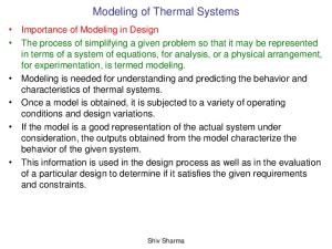
FIG. 1. Schematic figure of the surface-surface system out of thermal equilibrium. Here the two bodies occupy infinite half-spaces.
sons with the equilibrium results are done. We perform a detailed analysis of the relation between the surface-surface interaction when one body is rarefied 共surface-rarefied body force兲 and the surface-atom force. We also present a complete derivation and discussion of the recently predicted nonadditivity effects and asymptotic behaviors noted in 关23兴. We are interested in the force occurring between two planar bodies, which are kept at different temperatures and separated by a distance l. We consider that the bodies are thick enough, in order to exclude possible effects of the presence of the vacuum gap on the radiation outside the two bodies. We also assume that each body is in local thermal equilibrium, the whole system being in a stationary state. In our configuration the left-side body, 1, has a complex dielectric function 1共兲 = 1⬘共兲 + i1⬙共兲, occupies the volume V1 and is held at temperature T1. The right-side body, 2, has a complex dielectric function 2共兲 = 2⬘共兲 + i2⬙共兲, occupies the volume V2 and is held at temperature T2. First we assume that each body fills an infinite half-space, in particular V1 and V2 coincide with the left and right half-spaces, respectively. Later we consider a more general situation of two parallel thick slabs with the external regions shined by the thermal radiations at arbitrary temperatures. In this case additional distance-independent contributions to the pressure are present. Finally, we will consider the case in which one of the two bodies is rarefied. In this case the interplay between the finite thickness of the body and the nonequilibrium configuration leads to different interesting behaviors of the pressure. The general problem can be set in the following way, for two bodies occupying the two half-spaces. Let us choose the origin of the coordinate system at the boundary of the halfspace 1 and let us set the z axis in the direction of the halfspace 2 共see Fig. 1兲. The electromagnetic pressure between the two bodies along z can be calculated as 关30,31兴 Pneq共T1,T2,l兲 = 具Tzz共r,t兲典,
共2兲
1 1
1 1
1 1
⌳␣ 关E␣共r,t兲E共r,t兲 + B␣共r,t兲B共r,t兲兴, 8
1 1
1 1
1 1
1
1 1
1 1
1 1
1
1
1 1
1 1
1 1
1
1 1
1 1
1 1
1 1
1
1 1
1 1
1 1
1 1
1
1 1
1 1
1 1
1
1 1
1 1
1 1
1 1
1 1
1 1
1 1
1 1
1
1 1
1 1
1 1
1 1
1 1
1
1 1
1 1
1 1
1
1 1
1 1
1 1
1
1 1
1 1
1 1
1
1 1
1 1
1 1
1
1 1
1 1
1 1
1 1
1 1
1
1
1 1
1 1
1 1
1
1 1
1 1
1 1
1 1
1 1
1
1 1
1 1
1 1
1 1
1 1
1 1
1 1
1 1
1
1 1
1
1
1 1
1 1
1 1
1
1 1
1
1
1 1
1 1
1 1
1
1 1
1 1
1 1
10
1 1
1 1
1 10
10
1 1
1 1
10 10
1 1
1 1
10 10
10
1 1
1 10
10 10
1 1
1 10
10 10
10
1 1
10 10
10 10
10
1 10
10 10
10 10
10
10 10
10 10
10 10
10
10 10
10 10
10 10
10
10 10
10 10
10 10
10 10
10 10
10 10
10
10 10
10 10
10 10
10 10
10 10
10 10
10
10 10
10 10
10 10
10
10
10 10
10 10
10 10
10
10
10 10
10 10
10 10
10
10
10 10
10 10
10
10
10
10 10
10 10
1
1
1 1
1
1
1
Tzz共r,t兲 = − 1
1
1
1
1
1 1
1
1
1 1
1
1
1
1 1
1
1
1
1
1 1
1
1
1
1
1 1
1
1
2 1
1 1
1
1
1
1 1
1 1
1
1
1 1
1 1
1 1
1 1
1 1
1 1
1 1
1 1
1 1
1 1
1 1
1 1
1 1
1 10
1 1
1 1
10 10
1 1
1 10
10 10
1 1
10 10
10 10
1 1
10 10
10 10
1 10
10 10
10 10
10 10
10 10
10 10
10 10
10 10
10 10
10 10
10 10
10
10 10
10 10
10
10
10
10
10 10
10 10
10
10 10
10 10
10
10 10
10 10
10
10 10
10
10
10 10
10 10
10 10
10 10
10
10 10
10 10
10 10
10
10 10
10 10
10 10
10
10 10
10 10
10 10
10
10 10
10 10
10 10
10
10 10
10 10
10
10
10 10
10 10
10 10
10
10 10
10
10
10 10
10
1 10
10 10
10
10
10 10
10
10 10
10 10
10 10
10 10
10 10
10
10 10
10
10 10
10 10
10
10
10 10
10 10
10
10
10 10
10 10
10
10
10 10
10 10
10
10
10 10
10 10
10
10
10 10
10
10
10
10 10
10
10
10
1
1 1
1
1
1
1 1
1
1
1
1 1
1
1
1
1 1
1
1
1
1 1
1
1
1
1 1
1
1
1
1 1
1
1
1
1 1
1
1
1
1 1
1
1
1
1 1
1
1
1
1 1
1
1
1
1 1
1
1
1
1 1
1
1
1
1 1
1
1
1
1 1
1
1
1
1 1
1
1
1
1 1
1
1
1
1 1
1
1
1
1 1
1
1
1
1 1
1
1
1
1 1
1
1
1
1 1
1
1
1
1 1
1
1
1
1 1
1
1
1
1 1
1
1
1
1 1
1
1
1
1 1
1
1
1
1 1
1
1
1
1 1
1
1
1
1 1
1
1
1
1 1
1
1
1
1 1
1
1
1
1 1
1
1
1
1 1
10
1
1
1
共1兲
that should be regularized by subtracting the same expression at separation l → ⬁. In Eq. 共1兲, r is a generic point between the two bodies, and
is the zz component of the Maxwell stress tensor in the vacuum gap. Here ⌳␣ is a diagonal matrix with ⌳11 = ⌳22 = 1 and ⌳33 = −1. To calculate the pressure 共1兲 one must average over the state of the electromagnetic field the squares of the spatial components of the electric and magnetic field E共r , t兲 and B共r , t兲, which appear in Eq. 共2兲. Before starting with the analysis of the problem we mention the structure of this work in the following outline. In Sec. II we develop the formalism, introduce the role and the description of the fluctuations of the electromagnetic field, and specify the approach we adopt to deal with the surface optics. In Sec. III we recall the main results of the surfacesurface Casimir-Lifshitz interaction at thermal equilibrium, and in particular specify the distinction between the T = 0 共purely quantum兲 and the thermal contribution to the force, generated by the radiation pressure of the thermal radiation. In Sec. IV we present a detailed derivation of the surfacesurface pressure out of thermal equilibrium Pneq共T1 , T2 , l兲. In Sec. V we show an alternative and useful expression for Pneq共T1 , T2 , l兲, together with numerical results relative to particular couples of dielectric materials 共i.e., fused silicasilicon and sapphire-fused silica兲. In Sec. VI we deal with the distance-independent terms in the pressure due to the finite thickness of the two bodies, and the eventual effect of external radiation at different temperature impinging the external surfaces. In Sec. VII we derive the large distance behavior of the surface-surface pressure out of thermal equilibrium, and discuss the role of the propagating waves 共PW兲 and evanescent waves 共EW兲 contributions. We also make a comparison with the corresponding terms of the pressure at thermal equilibrium. In Sec. VIII we consider the interaction between a surface and a rarefied body and derive the large distance behaviors of the PW and EW components. In the same section we stress the presence of nonadditivity in the interaction out of equilibrium 共in contrast with the equilibrium case兲 and show the analysis of the crossing between different asymptotic behaviors. In Sec. IX we show the transition from the surface-rarefied body to surface-atom interactions out of thermal equilibrium, and demonstrate the essential role of finite thickness of the rarefied body. Finally, in Sec. X, we provide our conclusions. In Appendix A we give some details on the expression of the Green functions we used in our calculation and in Appendix B we discuss in detail the force acting between a surface and a rarefied body of finite thickness. II. FORMALISM
Our approach is based on the theory of the fluctuating electromagnetic 共EM兲 field developed by Rytov 关6兴. In this approach it is assumed that the field is driven by randomly fluctuating current density or, alternatively, by randomly fluctuating polarization field. In this respect the Maxwell equations become of Langevin-type. For a monochromatic field in a nonhomogeneous, linear, and nonmagnetic medium
022901-2
CASIMIR-LIFSHITZ FORCE OUT OF …
PHYSICAL REVIEW A 77, 022901 共2008兲
with the dielectric function 共 , r兲 the Maxwell equations become ∧ E关 ;r兴 − ikB关 ;r兴 = 0,
共3兲
∧ B关 ;r兴 + ik共 ;r兲E关 ;r兴 = − 4ikP关 ;r兴,
共4兲
where k = / c is the vacuum wave number and ∧ is the vector product symbol. The source of the electromagnetic fluctuations is described by the electric polarization P关 ; r兴, related to the electric current density as J关 ; r兴 = −iP关 ; r兴. We use the following notations for the frequency Fourier transforms A关 ; r兴 of the quantity A共t , r兲: A共t,r兲 =
冕
+⬁
−⬁
d −it e A关 ;r兴. 2
共5兲
To find the solution of the Maxwell equations we use the Green functions formalism. A Green function is a solution of the wave equation for a point source in presence of surrounding matter. When this solution is known one can construct the solution due to a general source using the principle of linear superposition. This method takes into account the effects of nonadditivity, which originates from the fact that the interaction between two fluctuating dipoles is influenced by the presence of a third dipole. Employing this formalism we can express the electric field at the observation point r as the convolution E关 ;r兴 =
冕
¯ 关 ;r,r⬘兴 · P关 ;r⬘兴dr⬘ . G
共6兲
Here P关 ; r⬘兴 is the random polarization at the source point ¯ 关 ; r , r⬘兴 is the dyadic Green function of the sysr⬘ and G tem. Then it is clear that the Green function plays the role of the response function in a linear-response theory. The Green function is the solution of the following equation 关32兴 ¯ 关 ;r,r⬘兴 = 4k2¯I␦共r − r⬘兲, 兵 ∧ ∧ − k2共,r兲其G
共7兲
where ¯I is the identity dyad. This equation, resulting from the Maxwell equations 共3兲 and 共4兲 and convolution 共6兲, has to be solved with proper boundary conditions characterizing the fields components at the interfaces, as well as the condition required by a retarded Green’s function 关35,36兴, i.e., ¯ 关 ; r , r⬘兴 → 0 as 兩r − r⬘兩 → ⬁. G Finally, it is useful to recall the relations G␣关 ; r , r⬘兴 * 关 ; r , r 兴 = G 关− ; r , r 兴 that are the = G␣关 ; r⬘ , r兴 and G␣ ⬘ ⬘ ␣ consequence of the microscopic reversibility in the linearresponse theory and the reality of the time dependent fields, respectively.
1 具E␣共r,t兲E共r⬘,t兲典sym ⬅ 具E␣共r,t兲E共r⬘,t兲 + E共r⬘,t兲E␣共r,t兲典. 2 共8兲 Notice that, although in this paper we are using symmetrized correlations, other possible forms of the correlation functions could be more appropriate in other situations 关33兴. The correlations 共8兲 in terms of their Fourier transforms can be presented as 具E␣共r,t兲E共r⬘,t兲典sym =
d d⬘ −i共−⬘兲t e 具E␣关 ;r兴E† 关⬘ ;r⬘兴典sym . 共9兲 2 2
Using Eq. 共6兲 these correlations can be expressed via the correlations of the polarization field P, which obeys the fluctuation-dissipation theorem 关30兴 具P␣关 ;r兴P† 关⬘ ;r⬘兴典sym =
冉 冊
ប⬙共,r兲 ប coth ␦共 2 2kBT − ⬘兲␦共r − r⬘兲␦␣ ,
共10兲
expressed via the Fourier transformed P关 ; r兴. Due to the presence of the ␦共r − r⬘兲 factor these fluctuations are local. Fluctuations of the sources in different points of the material are non-coherent. This permits to assume that in the nonequilibrium situation, when temperature T is different in different points, the sources correlations are given by the same equations. We must emphasize that this assumption, even being quite reasonable, is still a hypothesis, which is worth both of further theoretical investigation and experimental verification. The problem was discussed previously 共see particularly 关41兴兲, but in our opinion the conditions of applicability of the theory has not been still established. The same assumption was used by Polder and Van Hove 关28兴 to calculate the radiative heat transfer between two bodies with different temperatures. The assumption 共10兲 共local source hypothesis兲 represents the starting point of our analysis allowing for an explicit calculation of the electromagnetic field also if the system is not in global thermal equilibrium. It is now evident that EM field in the vacuum gap is given by the sum of the fields produced by the fluctuating polarizations in the materials filling respectively the half-space 1, with the dielectric function 1共兲 and temperature T1, and the half-space 2 with the dielectric function 2共兲 and temperature T2. Then the Fourier transform of the electric field correlations can be presented as 具E␣关 ;r兴E† 关⬘ ;r⬘兴典sym =
A. Field correlation functions
From Eq. 共1兲 it is evident that we are interested in the time correlations between different components of the electric 共magnetic兲 field at equal times. In the quantum theory such correlations are described by the averages of symmetrized products of the field components:
冕冕
冋
ប1⬙共兲 ប coth S共1兲 关 ;r,r⬘兴 2 2kBT1 ␣
+
ប2⬙共兲 ប coth 2 2kBT2
冉 冊 冉 冊
册
共2兲 ⫻S␣ 关 ;r,r⬘兴 ␦共 − ⬘兲,
共11兲
共i兲 共i = 1 , 2兲 is defined as convolution of two Green where S␣ functions
022901-3
PHYSICAL REVIEW A 77, 022901 共2008兲
ANTEZZA et al.
冕
共i兲 S␣ 关 ;r,r⬘兴 =
Vi
* dr⬙G␣␥关 ;r,r⬙兴G␥ 关 ;r⬙,r⬘兴. 共12兲
Here V1 and V2 are the volumes occupied by the left and right body, respectively, and the two terms in Eq. 共11兲 correspond to the parts of the pressure generated by the sources in each body separately. It is interesting to see how the global equilibrium is restored when T1 → T2 = T in Eq. 共11兲. In this case Eq. 共11兲 can be written as 具E␣关 ;r兴E† 关⬘ ;r⬘兴典sym =
Here the electric and magnetic contributions to the total pressure are explicit, and r is a point inside of the vacuum gap. The stress tensor is in fact constant in the vacuum gap due to the momentum conservation required by a stationary configuration 共see discussion in Sec. IV A兲. In this equation we omitted the symmetrization index since the average is taken at the same point r = r⬘. Using Eq. 共3兲 it is useful to rewrite expression 共17兲 in terms of the electric fields only 关34兴 as Pneq共T1,T2,l兲 = −
冉 冊
ប ប coth ␦ 共 − ⬘兲 2 2kBT ⫻
冕
冉
⍀
* dr⬙⬙共,r⬙兲G␣␥关 ;r,r⬙兴G␥ 关 ;r⬙,r⬘兴
= 4 Im G␣关 ;r,r⬘兴,
共14兲
具E␣关 ;r兴E† 关⬘ ;r⬘兴典sym
冉 冊
ប Im G␣关 ;r,r⬘兴␦共 − ⬘兲. 2kBT
Notice that all fluctuations presented in this section include both the vacuum 共T = 0兲 and the thermal fluctuations. These can be identified with the first and second terms, respectively, of the right-hand side 共RHS兲 of the identity
冉
冉 冊
冊
2 ប = sgn共兲 1 + ប兩兩/k T , B −1 2kBT e
The pressure 共1兲 can be presented in terms of the Fourier transformed fields correlations: 1 8
冕冕
neq neq Pneq th 共T1,T2,l兲 = Pth 共T1,0,l兲 + Pth 共0,T2,l兲.
d d⬘ −i共−⬘兲t e 2 2
⫻ ⌳␣兩关具E␣关 ;r兴E† 关⬘ ;r⬘兴典 + 具B␣关 ;r兴B† 关⬘ ;r⬘兴典兴兩r=r⬘ .
共17兲
共20兲
共21兲
The pressure at thermal equilibrium Peq共T , l兲, being a particular case of Eq. 共20兲, can be written as 共22兲
Peq th 共T , l兲
are given by Eq. 共18兲, The pressures P0共l兲 and where the field fluctuations are provided by Eq. 共15兲 after the substitution, respectively, of
冉 冊 冉 冊
ប → sgn共兲, 2kBT
共23兲
2 sgn共兲 ប → ប兩兩/k T . B −1 2kBT e
共24兲
coth
coth
B. Pressure in terms of fluctuations
共19兲
where the contribution of the zero-point 共T = 0兲 fluctuations, P0共l兲, is separated from that produced by the thermal fluctuations, Pneq th 共T1 , T2 , l兲. Furthermore, thanks to Eq. 共11兲 it is possible to express the thermal component of the pressure acting between the bodies as the sum of two terms
⫽ 0. 共16兲
Pneq共T1,T2,l兲 = −
冊
selects the electric and magnetic contributions, given by the first and the second term in Eq. 共19兲, respectively. From Eq. 共16兲 it is possible to express the total pressure as the sum
Peq共T,l兲 = P0共l兲 + Peq th 共T,l兲. 共15兲
coth
1 ⑀␣␥␦⑀␥⬘ k2
Pneq共T1,T2,l兲 = P0共l兲 + Pneq th 共T1,T2,l兲,
where ⍀ is a volume restricted by a surface where the Green function vanishes. Keeping in mind that in the vacuum gap ⬙ = 0, one can extend the integration in Eq. 共13兲 over the the whole space and using Eq. 共14兲 one recovers the well-known form of the electric fields fluctuation-dissipation theorem 关32兴 valid at a global thermal equilibrium:
= 2ប coth
⌰␦ = ⌳␣ ␦␣␦␦ +
共13兲
The integral over the product of two Green functions is connected with the imaginary part of the single Green function by the important 关41,42兴 relation
冕
d d⬘ −i共−⬘兲t e 2 2
Here the pressure is expressed in terms of the correlations 共11兲, and the operator
V1+V2
⫻G␥关 ;r⬙,r⬘兴.
冕冕
⫻ ⌰␦兩关具E␦关 ;r兴E†关⬘ ;r⬘兴典兴兩r=r⬘ . 共18兲
dr⬙⬙共,r⬙兲G␣␥关 ;r,r⬙兴
*
1 8
If one simply performs such substitutions, it is well known that Eq. 共18兲 diverges at T = 0, and contains constant 共l-independent兲 terms in the thermal part. The divergence has the same origin as the usual divergence of the zero-point fields energy in quantum electrodynamics, while the constant terms are related to the fact that we consider infinite bodies, and hence we neglect the pressure of the radiation exerted on the remote, external surfaces of the two bodies. To recover the exact finite value for the pressures P0共l兲, and exclude the constant terms in Peq th 共T , l兲, one should regularize the Green function in the RHS of Eq. 共15兲 by subtracting the bulk part Gbu ij , corresponding to a field produced by a pointlike dipole in an homogeneous and infinite dielectric 关7,39,40兴. In fact,
022901-4
CASIMIR-LIFSHITZ FORCE OUT OF …
PHYSICAL REVIEW A 77, 022901 共2008兲
the Green function with both the observation point r and the source point r⬘ in the vacuum gap 共see Appendix A 1兲 is given by the sum bu Gij关 ;r,r⬘兴 = Gsc ij 关 ;r,r⬘兴 + Gij 关 ;r,r⬘兴
共25兲
of a scattered and a bulk term. The subtraction of the bulk term corresponds to the subtraction of the pressure at l → ⬁, as prescribed after Eq. 共1兲. The expressions for the pressure at thermal equilibrium are given explicitly in Sec. III. Concerning the thermal pressure out of thermal equilibneq 共T1 , T2 , l兲 of Eq. 共20兲, it can be obtained from Eq. rium Pth 共18兲 by using Eq. 共11兲 and the substitution 共24兲. Also in this case the thermal pressure Pneq th 共T1 , T2 , l兲 contains an l-dependent and a constant term, as it happens for Peq th 共T , l兲 before being regularized. Differently from the equilibrium case, here the origin of the constant terms is not only due to the absence of the pressure acting on the remote surfaces, but is also related to the fact that out of thermal equilibrium there is a net momentum transfer between the bodies. In this case the constant terms can remain also after considering bodies of finite thickness, and can even be different for the two bodies, depending on the external radiations. In Secs. IV and V we will calculate Pneq th 共T1 , T2 , l兲 for two bodies filling two infinite half-spaces, and we will mainly discuss the pure l-dependent component. The constant terms will be discussed in Sec. VI for the general case of bodies of finite thickness, with impinging the external radiations at different temperatures. C. Electromagnetic waves in surface optics
In this work we formulate the electromagnetic problem in terms of s- and p-polarized vector waves and in terms of the Fresnel coefficients for the interfaces 关37兴. Such notations are very useful in surface optics. We will also employ the angular spectrum representation for the description of the EM and polarization vectors. If xˆ , yˆ , and zˆ are the coordinate unit vectors 共with real norm equal to 1兲, one can write the position vector as r = R + zzˆ , where the capital letter refers to vectors parallel to the interface 关R ⬅ 共Rx , Ry , 0兲兴. Let us write the electromagnetic 共complex兲 wave vector in the medium m with the complex dielectric function m共兲 = m ⬘ 共兲 + im⬙ 共兲 as q共m兲共⫾兲 = Q ⫾ qz共m兲zˆ .
共27兲
is a complex number with a positive imaginary part, with positive real part in case Im qz共m兲 = 0. Real and imaginary parts of qz共m兲 are expressed by the following relations: Re qz共m兲 =
冑
冑
1 ⬘ 共兲k2 − Q2兴其, 共28兲 兵兩m共兲k2 − Q2兩 + 关m 2
1 ⬘ 共兲k2 − Q2兴其. 共29兲 兵兩m共兲k2 − Q2兩 − 关m 2
Then, if the medium m is nonabsorbing 共m ⬙ = 0兲, for Q 艋 冑 m ⬘ k the wave vector qz共m兲 is real and corresponds to a wave propagating in the medium m, while for Q ⬎ 冑m ⬘ k the wave vector qz共m兲 is imaginary and corresponds to evanescent wave in the medium m. The following identities will be useful:
⬙ 共兲, 2 Im qz共m兲 Re qz共m兲 = k2m
共30兲
* 共Q2 + 兩qz共m兲兩2兲Re qz共m兲 = k2 Re关m 共兲qz共m兲兴,
共31兲
* 共兲qz共m兲兴. 共Q2 − 兩qz共m兲兩2兲Im qz共m兲 = k2 Im关m
共32兲
共m兲
It is worth noticing that the wave vectors q 共⫾兲 lie in the ˆ and zˆ . Then one can introplane of incidence spanned by Q duce the s- and p-unit complex polarization vectors ˆ ∧ zˆ , es共m兲共⫾兲 = Q 共m兲 ˆ 共m兲共⫾兲 = e共m兲 p 共⫾兲 = es 共⫾兲 ∧ q
共33兲 ˆ Qzˆ ⫿ qz共m兲Q
冑m共兲k
,
共34兲
that are vectors transversal and longitudinal to that plane, respectively. Usually the polarization vector es共m兲共⫾兲 关e共m兲 p 共⫾兲兴 is called transverse electric 共TE兲 关transverse magnetic 共TM兲兴 since it corresponds to the electric 共magnetic兲 field transverse to the plane of incidence. Our geometry consists of two half-spaces labeled with m = 1 , 2 separated by a vacuum gap. Inside of the gap the wave vector q and the polarization vectors e共⫾兲 are not labeled and are obtained, respectively, from the definitions 共26兲, 共27兲, 共33兲, and 共34兲 by omitting the apices 共m兲, and setting m = 1. Finally we can introduce the well known reflection and transmission Fresnel coefficients for the vacuum gapdielectric interfaces, which for the s- and p-wave components are s = rm
共26兲
Here the sign 共⫹兲 corresponds to an upward-propagating 共or evanescent兲 wave, and the sign 共⫺兲 corresponds to a downward-propagating 共or evanescent兲 wave. The vector Q ⬅ 共Qx , Qy , 0兲 is the projection 共always real兲 of q共m兲共⫾兲 on the interface and the z component of the wave vector, and qz共m兲 = 冑mk2 − Q2 ,
Im qz共m兲 =
s tm =
qz − qz共m兲
共m兲 ,
qz + qz 2qz共m兲
qz共m兲 + qz
,
rmp =
tmp =
qzm − qz共m兲 qzm + qz共m兲
共35兲
,
2冑m共兲qz共m兲 qz共m兲 + qzm共兲
.
共36兲
In particular, the coefficients rm relate the radiation in the vacuum gap impinging the interface m and its part reflected back into the vacuum gap. The coefficients tm relate the radiation impinging the interface m from the interior of the dielectric m and its part transmitted into the vacuum gap 共see Appendix A兲. III. PRESSURE AT THERMAL EQUILIBRIUM
In this section, we briefly recall the main results of the pressure in a system at thermal equilibrium. We present the
022901-5
PHYSICAL REVIEW A 77, 022901 共2008兲
ANTEZZA et al.
thermal component of the pressure as the sum of PW and EW components, and in terms of real frequencies, which will prove useful for the rest of the discussion. The results we show for the pressure at equilibrium are regularized 关see discussion after Eq. 共24兲兴. The Lifshitz surface-surface pressure at thermal equilibrium can be expressed in terms of real frequencies as Peq共T,l兲 = −
冕 冋冕
⬁
ប 22
冉 冊
d coth
0
⫻ Re
⬁
ប 2kBT
册
dQ Qqzg共Q, 兲 ,
0
共37兲
where g共Q, 兲 =
兺 =s,p
r1r2e2iqzl = 兺 关共r1r2兲−1e−2iqzl − 1兴−1 . D =s,p 共38兲
In the previous equation the multiple reflections are described by the factor D = 1 − r1r2e2iqzl ,
T ⬅
k BT P 共T,l兲 = 16l3
冕
⬁
dx x
2
0
⬁
k BT + 3 兺 3n c n=1
冕
⬁
冋
共10 + 1兲共20 + 1兲 x e −1 共10 − 1兲共20 − 1兲
共39兲
dp p2g共p,in兲,
册
−1
⫻ ប 2 ⫻
共40兲
冕
⬁
兺
d
兺
⬁
d
0
=s,p
0
=s,p
冕
1 e
ប/kBT
k
dQ Qqz
0
Re共r1r2e2iqzl兲 − 兩r1r2兩2 , 兩D兩2 1
e
−1
冕
ប/kBT
−1
冕
共43兲
⬁
dQ Q Im qze−2l Im qz
k
Im共r1r2兲 . 兩D兩2
共44兲
1
where p = 冑 The dielectric functions that enter to g共p , in兲 must be evaluated at imaginary frequencies 1,2 = 1,2共in兲, where n = 2kBTn / ប. In the first term of Eq. 共40兲 we have also introduced the static values of the dielectric functions 10 = 1共0兲 and 20 = 2共0兲. The pressure at thermal equilibrium includes contributions from zero-point fluctuations P0共l兲 and from thermal fluctuations Peq th 共T , l兲 as Eq. 共22兲 shows. P0共l兲 can be extracted from Eq. 共37兲 with the substitutes Eq. 共23兲 or from Eq. 共40兲 as the limit of continuous imaginary frequency. The final result for the T = 0 pressure is ប 2 2c 3
ប 2
共T,l兲 = − Peq,PW th
共T,l兲 = Peq,EW th
1 + c2Q2 / 2n.
P0共l兲 =
共42兲
which at room temperature is ⬇7.6 m. Then, the zero-point fluctuations dominate over the thermal contribution at small distances l Ⰶ T. In this limit behavior of the pressure is determined by the characteristic length scale opt Ⰶ T. In the interval opt Ⰶ l Ⰶ T one enters the Casimir-Polder regime where the pressure decays like 1 / l4. For distances l Ⰶ opt the force instead exhibits the 1 / l3 van der Waals–London dependence. The possibility of identifying the Casimir-Polder regime depends crucially on the value of the temperature. The temperature should be in fact sufficiently low in order to guarantee the condition T Ⰷ opt. The last part of this section focuses on the thermal component of the pressure that will often be used along the rest of the paper. The pressure Peq th 共T , l兲 can be obtained from Eq. 共37兲 by using 共24兲. Since such a component of the pressure will be compared with that out of thermal equilibrium, we show here explicitly its expression for PW and EW contributions:
for the vacuumand the reflection Fresnel coefficients rm dielectric interfaces are defined in Eq. 共35兲. By performing the Lifshitz rotation on the complex plane it is possible to write Eq. 共37兲 in terms of imaginary frequencies: eq
បc , k BT
冕 冕 ⬁
0
d
⬁
dp p23g共p,i兲.
共41兲
1
The pressure P0共l兲 admits two important limits, i.e., the van der Waals–London and the Casimir-Polder behaviors, valid at small and large distances, respectively, in respect to the characteristic length scale opt fixed by the absorption spectrum of the bodies 共typically is of the order of fraction of microns兲. The behavior of the thermal component Peq th 共T , l兲 is related to a second length scale, i.e., the thermal wavelength
In particular at high temperatures, or equivalently at large distances defined by the condition l Ⰷ T ,
共45兲
the leading contribution to the pressure is given by the expression for the total force 关7兴 Peq th 共T,l兲 =
k BT 16l3
冕
⬁
0
dx x2
冋
10 + 1 20 + 1 x e −1 10 − 1 20 − 1
册
−1
. 共46兲
It corresponds to the first term in Eq. 共40兲 and is entirely due to the thermal fluctuations of the EM field. In Ref. 关7兴 the asymptotic behavior 共46兲 has been found after the contour rotation in the complex plane of the EW term 共44兲, that is partially canceled by the PW term 共43兲. One can note that in this regime only the static value of the dielectric functions is relevant. The pressure 共46兲 is proportional to the temperature and is independent from the Planck constant as well as from the velocity of light. We will call this equation the Lifshitz limit. The pressure 共46兲 can be obtained from the thermal free energy F = E − TS of the electromagnetic field 共per unit area兲 according to the thermodynamic identity P = −共F / l兲T, where E and S are the thermal
022901-6
CASIMIR-LIFSHITZ FORCE OUT OF …
PHYSICAL REVIEW A 77, 022901 共2008兲
energy and entropy, respectively. It is interesting to note that, differently from the free energy, the thermal energy E decreases exponentially with l, which means that the pressure 共46兲 has pure entropic origin 关38兴. It is important that at large separations only the p polarization contributes to the force 共see, for example, in 关24兴, the detailed derivation of the PW and EW components兲. The reason is that for low frequencies the s-polarized field is nearly pure magnetic, but the magnetic field penetrates freely into a nonmagnetic material 关43兴. In the limit 10 , 20 → ⬁ we find the force between two metals k BT 共T,l兲 = 共3兲. Peq,met th 8l3
共47兲
Let us empathize that this result was obtained for interaction between real metals 关44兴. For “ideal mirrors” considered by Casimir, both polarizations of electromagnetic fields are reflected. In this case there will be an additional factor 2 in Eq. 共46兲 due to the contribution of the s polarization. This ideal case can be realized using superconducting mirrors. It is useful to note that the surface-surface pressure Peq共T , l兲 given by the Lifshitz result 共40兲 hides a nontrivial cancellation between the components of the pressure related to real and imaginary values of the EM wave vectors, leading, respectively, to the propagating 共PW兲 and evanescent 共EW兲 wave contributions 关17,45兴. This study deserves careful investigation since for a configuration out of thermal equilibrium such cancellations are no longer present, and the PW and EW contribution will provide different asymptotic behaviors. The new effect, as we will see, is particularly important if one of the two bodies is a rarefied gas.
pressure is calculated for two infinite bodies 共see discussion at the end of Sec. II B兲. A. S functions
In this subsection we show the result for the tensors S␦共1兲 and S␦共2兲 defined by Eq. 共12兲. In terms of the lateral Fourier transforms s␦共1兲 关 ; Q , z1 , z2兴 and s␦共2兲 关 ; Q , z1 , z2兴 one has S␦关 ;r1,r2兴 =
es共m兲共⫾兲 = 共兩sin 兩,− cos sin /兩sin 兩,0兲, e共m兲 p 共⫾兲 =
冕
⬁
0
d
e
1⬙共兲 ប/kBT
⫻Re兩关⌰␦S␦共1兲 关 ;r1,r2兴兴兩r1=r2 ,
cos , ⫿ qz共m兲 sin ,Q兲.
Q2 + 兩qz共m兲兩2 . 兩m兩k2
2 兩e共m兲 p 共⫾兲兩 =
共51兲
共52兲
After explicit calculation using the Green function given in Appendix A we find for the s␦共1兲 and s␦共2兲 functions the explicit expressions s␦共1兲 关 ;Q,z1,z2兴 =
42k2 Re qz共1兲 1⬙共兲
兩t兩2
兺 1 兩e共1兲共+ 兲兩2 兩q共1兲兩2 =s,p 兩D兩2 z
*
⫻关e,␦共+ 兲e* ,共+ 兲ei共qzz1−qz z2兲 *
*
+ e,␦共+ 兲e* ,共− 兲ei共qzz1+qz z2兲e−2iqz lr2* *
+ e,␦共− 兲e* ,共+ 兲e−i共qzz1+qz z2兲e2iqzlr2 *
+ e,␦共− 兲e* ,共− 兲e−i共qzz1−qz z2兲 ⫻e−4 Im qzl兩r2兩2兴,
共48兲
where r1 = r2 is a point in the vacuum gap and the function S is defined in Eq. 共12兲. In Eq. 共48兲 we used the parity properties ⬙共兲 = −⬙共−兲 and S␦关 ; r1 , r2兴 = S␦*关− ; r1 , r2兴 to restrict the range of integration to the positive frequencies. It is evident that Pneq th 共0 , T , l兲 can be expressed similarly to Eq. 共48兲, but with 1⬙共兲 → 2⬙共兲 and S␦共1兲 → S␦共2兲 . Below we specify the expressions of the tensors S␦共1兲 and 共2兲 S␦ 共Sec. IV A兲, calculate the electric and magnetic contributions to the pressure 共Sec. IV B兲, and finally provide the result for the total pressure in terms of PW and EW components 共Sec. IV C兲. The total pressure will be rewritten in a different form in Sec. V by using a powerful expansion in multiple reflections. In the present and in the next Sec. V the
共m兲
共50兲
Here it is evident that 兩es共m兲共⫾兲兩2 = 1 and
s␦共2兲 关 ;Q,z1,z2兴 =
−1
1
冑mk 共⫿qz
As was discussed above 关see Eqs. 共11兲 and 共21兲兴 each body contributes separately to the thermal pressure. In particular, the pressure resulting from the thermal fluctuations in the body 1 is ប 163
d2Q iQ·共R −R 兲 1 2 s 关 ;Q,z ,z 兴. 共49兲 e ␦ 1 2 共2兲2
By choosing the x axis parallel to the vector D = R1 − R2 and defining as the angle between Q and D one gets that Qx = Q cos , Qy = Q sin and the polarization vectors become
IV. PRESSURE OUT OF THERMAL EQUILIBRIUM BETWEEN TWO INFINITE DIELECTRIC HALF-SPACES
Pneq th 共T,0,l兲 = −
冕
42k2 Re qz共2兲 2⬙共兲 兩qz共2兲兩2
e−2l Im qz
共53兲 兩t兩2
兺 2 2 兩e共2兲共− 兲兩2 =s,p 兩D兩 *
⫻ 关e,␦共− 兲e* ,共− 兲e−i共qzz1−qz z2兲 *
+ e,␦共− 兲e* ,共+ 兲e−i共qzz1+qz z2兲r1* *
+ e,␦共+ 兲e* ,共− 兲ei共qzz1+qz z2兲r1 *
+ e,␦共+ 兲e* ,共+ 兲ei共qzz1−qz z2兲兩r1兩2兴,
共54兲
where D is defined in Eq. 共39兲. It is worth noticing that in the nonequilibrium but stationary regime the fields correlation functions s共1,2兲 are not uniform in the vacuum cavity, while on the contrary the Maxwell stress tensor Tzz 共which is related to the momentum flux兲 has the same value in each point of the vacuum gap. This is valid also at equilibrium, and is a direct consequence of the momentum conservation required by a stationary con-
022901-7
PHYSICAL REVIEW A 77, 022901 共2008兲
ANTEZZA et al.
figuration. To show this property one can set z1 = z2 = z in Eq. 共53兲, where the dependence on z appears only in the exponential factors 关the same would happen for Eq. 共54兲兴. Let us note that now the first and the last terms in such an expression are proportional to e2z Im qz and e−2z Im qz, respectively, while the second and the third terms are proportional to e−2iz Reqz and e2iz Reqz, respectively. As it will be clear in the next Sec. IV B the first and the last terms will be responsible for the PW contribution to the pressure 共for which Im qz = 0兲, while the second and the third terms will be responsible for the EW contribution 共for which Re qz = 0兲. It is then evident that the position z disappears in the Maxwell stress tensor. B. Electric and magnetic contributions to the pressure
The pure electric contribution to the pressure Pneq th 共T , 0 , l兲 is due to the first term in Eq. 共19兲 ⌳␣␦␣␦␦S␦共1兲 兩关 ;r1,r2兴兩r1=r2,z1=0
冕 ⬙
2k2 1 ⫻
冋
⬁
dQ Q
0
−
冉
=
1 k2
冕
0
dQ Q 2
冕
0
0
兩qz共1兲兩2
兩ts1兩2 关共q2 + 兩qz兩2兲共1 + 兩rs2兩2e−4 Im qzl兲 + 2共qz2 兩Ds兩2 z 兩t1p兩2 Q2 + 兩qz共1兲兩2 2 关共qz 兩D p兩2 兩1共兲兩k2
共57兲
冋
冕
⬁
d
0
1 eប/kBT − 1
冕
k
dQ Q
0
Re qz共1兲 兩qz共1兲兩2
qz2
册
兩ts1兩2 兩t1p兩2 Q2 + 兩qz共1兲兩2 s 2 共1 + 兩r 兩 兲 + 共1 + 兩r2p兩2兲 , 2 兩Ds兩2 兩D p兩2 兩1共兲兩k2 共58兲
共T,0,l兲 Pneq,EW th =− 共55兲 ⫻
ប 22
冋
冕
⬁
d
0
1 eប/kBT − 1
冕
⬁
dQ Q
k
Re qz共1兲 兩qz共1兲兩2
qz2e−2l Im qz
册
兩ts1兩2 兩t1p兩2 Q2 + 兩qz共1兲兩2 s Re共r2p兲 . 2 Re共r2兲 + 兩Ds兩 兩D p兩2 兩1共兲兩k2
共59兲
Now, using helpful identities 关46兴
1 ⌳␣⑀␣␥␦⑀␥⬘ S␦共1兲 兩关 ;r1,r2兴兩r1=r2,z1=0 k2 2
ប 42
⫻
while the magnetic contribution is related by the second term in Eq. 共19兲, and is given by
⬁
Re qz共1兲
From this general expression one can extract the contribution of the propagating waves 共PW兲 in the empty gap, for which qz is real and hence qz2 = 兩qz兩2, and the contribution of the evanescent waves 共EW兲, for which qz is pure imaginary and hence qz2 = −兩qz兩2:
兩qz兩2 − Q2 兩t1p兩2 共1兲 2 2 兩e p 共+ 兲兩 兩D p兩 k2
,
冕
dQ Q
冎
=−
冊册
eប/kBT − 1
⬁
− 兩qz兩2兲Re共r2pe2iqzl兲兴 .
兩qz共1兲兩2
兩qz兩 − Q p 2 −4l Im q z + 兩r2兩 e k2
0
1
Pneq,PW 共T,0,l兲 th
兩qz兩2 + Q2 p* −2iq*l 兩qz兩2 + Q2 p 2iq l r2 e z − r2 e z k2 k2 2
d
+ 兩qz兩2兲共1 + 兩r2p兩2e−4 Im qzl兲 + 2共qz2
兩ts1兩2 共1兲 * s 兩e 共+ 兲兩2共1 + r2*e−2iqz l + rs2e2iqzl 兩Ds兩2 s
2
冕
⬁
− 兩qz兩2兲Re共rs2e2iqzl兲兴 +
Re qz共1兲
+ 兩rs2兩2e−4l Im qz兲 +
再
⫻
共1兲 共1兲 共1兲 = 兩关S11 + S22 − S33 兴兩r1=r2,z1=0
=
ប 82
neq Pth 共T,0,l兲 = −
Re qz共1兲兩ts1兩2
d iQD cos e 兩兵33⬘共s11 + s22兲 2
兩qz共1兲兩2
=
Re qz共1 − 兩rs1兩2兲 + 2 Im qz Im rs1 , 兩qz兩2
+ 关Q 共s33 − s22 − s11兲 + Q2x s11 + Q2y s22 + QxQy共s12 + s21兲兴
Re关1*共兲qz共1兲兴兩t1p兩2
+ 关i3共Qys23 + Qxs13兲 − i3⬘共Qys32 + Qxs31兲兴其兩D=0,z1=z2=0 ,
兩1共兲兩兩qz共1兲兩2
2
=
共60兲
Re qz共1 − 兩r1p兩2兲 + 2 Im qz Im r1p , 兩qz兩2
共56兲
共61兲
where s = s共1兲. One can show that, as it happens for the equilibrium case, the magnetic contribution 共56兲 coincides with the electric one 共55兲, after the interchange of the polarization indexes s ↔ p.
and similar ones for 1 ↔ 2, it is possible to express 共T , 0 , l兲 and Pneq,EW 共T , 0 , l兲 as Pneq,PW th th 共T,0,l兲 = − Pneq,PW th
C. Final expression for the pressure
Taking the sum of Eqs. 共55兲 and 共56兲 one finds that the pressure Pneq th 共T , 0 , l兲 in Eq. 共48兲 is 022901-8
⫻
ប 42
冕
兺 =s,p
⬁
0
d
1 eប/kBT − 1
冕
k
dQ Qqz
0
共1 − 兩r1兩2兲共1 + 兩r2兩2兲 , 兩D兩2
共62兲
CASIMIR-LIFSHITZ FORCE OUT OF …
Pneq,EW 共T,0,l兲 = th
ប 2
冕
⬁
0
d
1 e
ប/kBT
⫻Im qze−2l Im qz
−1
兺 =s,p
PHYSICAL REVIEW A 77, 022901 共2008兲
冕
⬁
dQ Q
k
Im共r1兲Re共r2兲 . 兩D兩2 共63兲
Note that the PW term 共62兲 contains a distance independent contribution that will be discussed in the next section. The pressure Pneq th 共0 , T , l兲 can be obtained following the same procedure but using the function s共2兲 ij given by Eq. 共54兲. The result can be obtained without calculation simply by the interchange r1 ↔ r2 in Eqs. 共62兲 and 共63兲. V. ALTERNATIVE EXPRESSION FOR THE PRESSURE
The thermal pressure between two bodies in a configuration out of thermal equilibrium was derived in the previous section, and expressed in terms of Eqs. 共62兲 and 共63兲. In this section we present an alternative expression for such a pressure, explicitly in terms of the pressure at thermal equilibrium. In Sec. V A we discuss the case of bodies made of identical materials 1 = 2, in Sec. V B we discuss the general case of bodies made of different materials, and finally in Sec. V C we show numerical results for the pressure between different bodies held at different temperatures.
identical bodies. It can be done using Eq. 共21兲 where neq Pneq th 共T , 0 , l兲 is given by Eqs. 共62兲 and 共63兲, and Pth 共0 , T , l兲 is neq obtained from Pth 共T , 0 , l兲 after the interchange r1 ↔ r2. In Pneq th 共T , 0 , l兲 we can separate symmetric and antisymmetric parts in respect to permutations of the bodies 1 ↔ 2. The factors sensitive to such a permutations in Eqs. 共62兲 and 共63兲 are, respectively, 共1 − 兩r1兩2兲共1 + 兩r2兩2兲 = 共1 − 兩r1r2兩2兲 + 共兩r2兩2 − 兩r1兩2兲, 共65兲 Im共r1兲Re共r2兲 =
共66兲 where we omitted the index . The symmetric parts, 共1 − 兩r1r2兩2兲 for PW and Im共r1r2兲 / 2 for EW, are responsible for eq the equilibrium term Pth 共T , l兲 / 2 in the nonequilibrium pressure as Eq. 共64兲 shows. Concerning the EW terms, if one takes the symmetric part of Eqs. 共63兲, one obtains exactly 共T , l兲 / 2, where Peq,EW 共T , l兲 coincides with the equilibPeq,EW th th rium EW component 共44兲. The analysis of the PW term is more delicate; in fact, if one takes the symmetric part 共1 共T , l兲 / 2, where − 兩r1r2兩2兲 of Eq. 共62兲, one obtains ¯Peq,PW th ¯Peq,PW共T,l兲 = − ប th 22
A. Pressure between identical bodies
In the case of two identical materials the pressure between bodies can be found without any calculations using the following simple consideration. Let the body 1 be at temperature T and the body 2 be at T = 0, then the thermal pressure will be Pneq th 共T , 0 , l兲. Because of the material identity the pressure will be the same if we interchange the temperatures of neq the bodies: Pneq th 共T , 0 , l兲 = Pth 共0 , T , l兲. In general, we know from Eq. 共21兲 that the thermal part of the pressure is given by the sum of two terms each of them corresponding to a configuration where only one of the bodies is at nonzero temneq neq perature, i.e., Pneq th 共T1 , T2 , l兲 = Pth 共T1 , 0 , l兲 + Pth 共0 , T2 , l兲. It is now evident that at equilibrium, where T1 = T2 = T, the latter eq equation gives Pneq th 共T , 0 , l兲 = Pth 共T , l兲 / 2 and we find for the total pressure Pneq th 共T1,T2,l兲 =
Peq th 共T1,l兲 2
+
Peq th 共T2,l兲 2
.
共64兲
Therefore, the pressure between identical materials is expressed only via the equilibrium pressures at T1 and T2. The same result was obtained by Dorofeyev 关25兴 by an explicit calculation of the pressure. It is interesting to note that Eq. 共64兲 is valid not only for the plane-parallel geometry, but for any couple of identical bodies of any shape displaced in a symmetric configuration with respect to a plane. B. Pressure between different bodies
It is convenient to present the general expression of the pressure in a form which reduces to Eq. 共64兲 in the case of
1 1 Im共r1r2兲 + 关Im共r1兲Re共r2兲 − Re共r1兲Im共r2兲兴, 2 2
⫻
冕
冕
⬁
0
d eប/kBT − 1
k
dQ Qqz
0
兺
=s,p
1 − 兩r1r2兩2 . 兩D兩2
共67兲
The above equation is different from Peq,PW 共T , l兲 given by th Eq. 共43兲. The difference has a clear origin. In fact the pressure out of equilibrium, from which Eq. 共67兲 is derived, is calculated for bodies occupying two infinite half-spaces. On the con共T , l兲 was obtained after trary the equilibrium pressure Peq,PW th proper regularization, and hence taking into account the pressure exerted on the external surfaces of bodies of finite thickness 关see discussion after Eq. 共24兲兴. Then the difference between Eqs. 共43兲 and 共67兲 is just a constant: 4 ¯Peq,PW共T,l兲 = Peq,PW共T,l兲 − 4T , th th 3c
共68兲
where = 2kB4 / 60c2ប3 is the Stefan-Boltzmann constant. Using the following multiple-reflection expansion of the factor 兩D兩−2:
冉
⬁
冊
1 1 1 + 2 Re 兺 Rne2inqzl , 2iqzl 2 = 兩1 − Re 兩 1 − 兩R兩2 n=1
共69兲
where R = r1r2, it is not difficult to show explicitly that Eqs. 共43兲 and 共67兲 are related by Eq. 共68兲. The constant term in Eq. 共68兲 comes from the first term of this expansion. Collecting together the symmetric and antisymmetric parts we can finally present the nonequilibrium pressure in the following useful form:
022901-9
PHYSICAL REVIEW A 77, 022901 共2008兲
ANTEZZA et al.
−
⌬PPW th 共T2,l兲,
共T1,l兲 Peq,EW 共T2,l兲 Peq,EW th + th + ⌬PEW th 共T1,l兲 2 2 共71兲
This is one of the main results of this paper. Here B共T1 , T2兲 = 2共T41 + T42兲 / 3c is a l-independent term, discussed in Eq. 共68兲. The equilibrium pressures Peq,PW 共T , l兲 and th Peq,EW 共T , l兲 are defined by Eqs. 共43兲 and 共44兲 and do not th contain l-independent terms. The expressions ⌬PPW 共T , l兲 and th ⌬PEW 共T , l兲 are antisymmetric with respect to the interchange th of the bodies 1 ↔ 2 and are defined as ប 42
⌬PPW th 共T,l兲 = − ⫻ ប 22 ⫻
冕
d
0
d
0
兺 =s,p
⬁
兺 =s,p
冕
⬁
1 eប/kBT − 1
冕
k
dQ Qqz
兩r2兩2 − 兩r1兩2 , 兩D兩2 1
eប/kBT − 1
冕
PW 共T兲 = − ⌬Pth,a
共72兲
⬁
dQ Q Im qze−2l Im qz
k
Im共r1兲Re共r2兲
− Im共r2兲Re共r1兲 . 兩D兩2
⫻
ប 42
兺
冕
=s,p ⬁
⬁
d
0
e
兩r2兩2 − 兩r1兩2 1 − 兩r1r2兩2
再冕
ប =− 兺 Re 22 n=1 ⫻
1 ប/kBT
⬁
0
兩r兩2 − 兩r兩2
d
−1
冕
共73兲
k
dQ Qqz
0
共74兲
,
1 eប/kBT − 1
2 1 n 2inq l 兺 2 共r1 r2 兲 e r 兩 1 − 兩r =s,p 1 2
1
1x10
1x10
−4
2
T = 0K , T = 300K (dashed) 1
2
−5
−6
1x10
1
2
3 separation [µm]
4
5
FIG. 2. Thermal component 共only l-dependent part兲 of the pressure out of equilibrium for fused silica-silicon system in the configuration 共T1 = 300 K, T2 = 0 K兲 共solid兲 and in the configuration 共T1 = 0 K, T2 = 300 K兲 共dashed兲. We plot also the thermal part of the force at thermal equilibrium at T = 300 K 共dotted兲.
0
Let us note that the EW term 共73兲 goes to 0 for l → ⬁ because evanescent fields decay at large distances. However, the PW term 共72兲 contains a l-independent component since in the nonequilibrium situation there is momentum transfer between bodies. This l-independent component can be directly extracted from Eq. 共72兲 using the expansion 共69兲. This expansion shows explicitly the contributions from multiple reflections. The distance independent term corresponds to the first term in the expansion 共69兲, and it is related with the radiation that pass the cavity only once, i.e., without being PW 共T , l兲 as the sum reflected. Finally it is possible to write ⌬Pth PW PW PW ⌬Pth 共T , l兲 = ⌬Pth,a共T兲 + ⌬Pth,b共T , l兲, where the constant and the pure l-dependent terms are respectively
PW ⌬Pth,b 共T,l兲
T1 = T2 = 300K (dotted) T = 300K , T = 0K (solid)
共70兲
− ⌬PEW th 共T2,l兲.
⌬PEW th 共T,l兲 =
1x10
Pressure [dine/cm2]
PW 共T1,l兲 ⌬Pth
+ 共T1,T2,l兲 = Pneq,EW th
−3
共T1,l兲 Peq,PW 共T2,l兲 Peq,PW th + th − B共T1,T2兲 2 2
Pneq,PW 共T1,T2,l兲 = th
z
冕
冎
k
dQ Qqz
0
.
共75兲
At thermal equilibrium T1 = T2 = T the sum of Eqs. 共70兲 and 共71兲 provides the Lifshitz formula except for the term −4T4 / 3c, which is canceled due to the pressure exerted on
the remote external surfaces of the bodies, as explicitly shown in the next section. Out of thermal equilibrium, but for identical bodies, r1 = r2, the antisymmetric terms disapEW pear: ⌬PPW th 共T , l兲 = ⌬Pth 共T , l兲 = 0. In this case, Eq. 共64兲 is reproduced. It is now clear that, due to the antisymmetric terms, Eq. 共64兲 is not valid if the two bodies are different. The problem of the interaction between two bodies with different temperatures was previously considered by Dorofeyev 关25兴 and Dorofeyev, Fuchs, and Jersch 关26兴. The authors used a different method, based on the generalized Kirchhoff’s law 关6兴. The general formalism of 关25兴 agrees with our Eqs. 共74兲 and 共75兲. However, our results are in disagreement with the results of 关26兴, where Eq. 共64兲 was found to be valid also for bodies of different materials, so that we argue that the results of the last paper were based on some inconsistent derivation. C. Numerical results for the pressure between two different bodies out of thermal equilibrium
In this section we show the results of the calculation of the pressure between two different bodies, for configurations both in and out of thermal equilibrium. In Figs. 2 and 3 we show the numerical results of the pressure for a system made of fused silica 共SiO2兲 for the left-side body 1 and low conductivity silicon 共Si兲 for the right-side body 2. In both cases the experimental values of the dielectric functions in a wide range of frequencies were taken from the handbook 关47兴. In particular in Fig. 2 we show the thermal pressure Pneq th 共T1 , T2 , l兲, sum of Eqs. 共70兲 and 共71兲, as a function of the separation l between 0.5 m and 5 m. Here we omit the l-independent terms. The pressure is presented for the configuration 共T1 = 300 K, T2 = 0 K兲 关solid line兴 and for the configuration 共T1 = 0 K, T2 = 300 K兲 关dashed兴. We plot also the thermal part of the force at thermal equilibrium, which is the sum of Eqs. 共43兲 and 共44兲, at the temperature T = 300 K 共dotted兲. The sum of the two configurations out of thermal equilibrium provides the force at thermal equilibrium. In Fig. 3 we show the relative contribution Pth / P0 of the thermal com-
022901-10
CASIMIR-LIFSHITZ FORCE OUT OF …
1
T1 = 300K , T2 = 0K (solid)
0.8
T1 = 0K , T2 = 300K (dashed)
Pth/P0
0
1
T1 = T2 = 300K (dotted)
0.8 0.6
th
P /P
PHYSICAL REVIEW A 77, 022901 共2008兲
0.4
0.2
0.2
2
3 separation [µm]
4
5
1
FIG. 3. Relative contribution of the thermal component of the pressure 共only l-dependent part兲 out of equilibrium for fused silicasilicon system in the configuration 共T1 = 300 K, T2 = 0 K兲 共solid兲, 共T1 = 0 K, T2 = 300 K兲 共dashed兲, and at thermal equilibrium at T = 300 K 共dotted兲.
ponent 共only the l-dependent terms兲 of the pressure with respect to the vacuum pressure P0共l兲 given by Eq. 共41兲. We performed the same analysis for a different couple of materials, and in particular we considered sapphire 共Al2O3兲 for the left-side body 1, and fused silica 共SiO2兲 for the rightside body 2. Also in this case the experimental values of the dielectric functions were taken from the handbook 关47兴. The results of such calculations are shown in Figs. 4 and 5, where the same quantities of Figs. 2 and 3 were plotted. From Figs. 2 and 3 it is evident that at small separations the pressure at 共T1 = 300 K, T2 = 0 K兲 is lower than that at 共T1 = 0 K, T2 = 300 K兲, and the situation is inverted at large separations. This is a characteristic feature of the materials we use. In fact for the sapphire-fused silica system we found the opposite behavior, as it is evident from Figs. 4 and 5. This behavior is the result of the interplay between the relevant frequencies in the problem, i.e., the thermal wavelength T, the separation l, and the different positions of the resonances in the dielectric functions for the different couples of materials.
1x10
−3
T = T = 300K (dotted) 1
2
1
2
Pressure [dine/cm ]
T = 300K , T = 0K (solid)
1x10
1x10
−4
2
T1 = 0K , T2 = 300K (dashed)
−5
−6
1x10
1
2
3 separation [µm]
4
5
FIG. 4. Same of Fig. 2, for the sapphire-fused silica system.
T1 = 0K , T2 = 300K (dashed)
0.6
0.4
1
T1 = T2 = 300K (dotted) T1 = 300K , T2 = 0K (solid)
2
3 separation [µm]
4
5
FIG. 5. Same as Fig. 3, for the sapphire-fused silica system. VI. PRESSURE BETWEEN TWO THICK SLABS
In Secs. IV and V we derived and discussed the nonequilibrium pressure between two materials filling two infinite half-spaces. We did not regularize the pressure, i.e., we did not consider the extra pressure due to the presence of the external surfaces of the bodies. This would simply add new l-independent terms. We focused mainly on the l-dependent part. In this section we fill this gap, and derive the exact constant terms of the pressure for the general case of two bodies of finite thicknesses at different temperatures, in the presence of external radiation. At thermal equilibrium, due to the momentum’s conservation theorem, the pressure cannot contain constant terms. In fact both Eqs. 共43兲 and 共44兲 go to zero as l goes to infinity. Here the regularization was performed by subtracting the bulk part of the full Green function 关see discussion after Eq. 共24兲兴. The inclusion of the bulk part would add an extra l-independent term −4T4 / 3c, as it is evident from the nonregularized Eq. 共68兲. Physically the origin of this extra term is due to the fact that the bodies are considered to be infinite and hence have no external surfaces. The presence of the external surfaces generates an extra pressure 4T4 / 3c, and finally the total pressure becomes l independent. It is worth noticing that at thermal equilibrium the force acting on one body is exactly the same 共apart from the sign兲 of that acting on the second body. Out of thermal equilibrium, for bodies occupying two half-spaces, one finds the nonregularized pressure given by the sum of Eqs. 共62兲 and 共63兲. In this case the pressure contains distance-independent components, and is the same on both materials 共apart from the sign兲. For bodies of finite thickness one should account for extra l-independent terms in the pressure due to the presence of two more interfaces between the bodies and the external regions 共see Fig. 6兲 where, in general, the radiation is not in equilibrium with the bodies. In this configuration the pressure acting on the body 1 can be different from that acting on the body 2. It should be noted that the new l-independent terms should be added to Eqs. 共70兲 and 共71兲, and originate from the PW waves only. Below we derive the result for such a general configuration by manipulating Eq. 共62兲.
022901-11
PHYSICAL REVIEW A 77, 022901 共2008兲
ANTEZZA et al.
1
⬅h 兩Pneq,PW 共0,Tbb,l兲兩1=1 =− th
2
2
Tbb1 ⬅h 共Th,0,l兲兩1=1 =− 兩Pneq,PW th
Tbb2 T1
l
2
T2
4 2Tbb − Pd共Tbb兲, 3c
共80兲
2T4h + Pd共Th兲, 3c
共81兲
where Pd共T兲 =
z
ប 42
冕
⬁
d
0
1 eប/kBT − 1
冕
k
dQ Qqz
0
兩rh兩2 , 兺 =s,p
FIG. 6. Schematic figure of the two-slab system out of thermal equilibrium.
Let us consider the case where both the bodies occupy thick slabs, as represented in Fig. 6. On the left of the body 1 impinges radiation at temperature Tbb1, while on the right of the body 2 impinges radiation at temperature Tbb2. Then the pressure acting on the body 1 and body 2 will be respectively: neq P1,th 共Tbb1,T1,T2,l兲 = Pneq th 共T1,T2,l兲 + PL共T1,Tbb1兲, 共76兲
共82兲 and rh are defined similar to Eq. 共35兲 but using the dielectric function h. Finally, we obtain the main result of this section, i.e., Eq. 共78兲 becomes PR共Th,Tbb兲 = −
4 兲 2共T4h + Tbb + Pd共Th兲 − Pd共Tbb兲. 共83兲 3c
In the same way it is possible to calculate PL共Th , Tbb兲 from Eq. 共79兲, and it is evident that the result will be PL共Th,Tbb兲 = − PR共Th,Tbb兲.
neq P2,th 共T1,T2,Tbb2,l兲 = − Pneq th 共T1,T2,l兲 + PR共T2,Tbb2兲.
共77兲 Pneq th 共T1 , T2 , l兲
Here is the pressure out of thermal equilibrium given by the sum of Eqs. 共62兲 and 共63兲 for materials filling infinite half-spaces. PL is the pressure due to the presence of a new left-side interface of the material 1 while PR is the pressure due to the presence of a new right-side interface of the material 2. Both PL and PR are constant terms and include two contributions: The pressure of the external radiation impinging on the outer interface and the back reaction produced by the emission of radiation from the body to the vacuum half-space. For thick enough slabs, it is possible to calculate the terms PL and PR using the expression of the pressure acting on a body h which occupies an infinite half-space. In general, it has a dielectric function h, is at temperature Th, and a thermal radiation with temperature Tbb impinges on its free surface. There are two possible configurations. One corresponds to the body h on the left and radiation impinging from the right, the second correspond to the body on the right and radiation impinging from the left. In the two cases the pressures can be expressed in terms of the pressure between two 共T1 , T2 , l兲 derived in the previous secinfinite bodies Pneq,PW th tion and are, respectively,
At equilibrium Th = Tbb = T we find that PR共T , T兲 = −PL共T , T兲 = −4T4 / 3c does not depend on material characteristics and coincides with the pressure of the blackbody radiation. It is also interesting to see that for a white-body 共W兲, corresponding to 兩rh兩2 = 1, and for a blackbody 共B兲, corresponding to 兩rh兩2 = 0, one obtains PR共0,T兲W = −
4T4 , 3c
PR共T,0兲W = 0,
PR共0,T兲B = −
PR共T,0兲B = −
2T4 , 3c
2T4 . 3c
共85兲
共86兲
From these relations one can see that PR共0 , T兲W / PR共0 , T兲B = 2, as it should be for the radiation pressure. Furthermore, one has that PR共T , 0兲W = 0. This is the consequence of the fact that 兩rh兩2 = 1 the radiation impinging on the surface from the interior of the material is fully reflected and there is no flux of momentum outside the body. In the particular case when the external radiation is at equilibrium with the corresponding body, i.e., Tbb1 = T1 and Tbb2 = T2, from Eqs. 共83兲 and 共84兲 one obtains that Eqs. 共76兲 and 共77兲 become respectively
⬅h , 共0,Tbb,l兲 + Pneq,PW 共Th,0,l兲兴兩1=1 PR共Th,Tbb兲 = 兩关Pneq,PW th th 2
neq neq P1,th 共Tbb1 = T1,T1,T2,l兲 = Pth 共T1,T2,l兲 +
共78兲 ⬅h 共Tbb,0,l兲 + Pneq,PW 共0,Th,l兲兴兩2=1 . PL共Th,Tbb兲 = 兩 − 关Pneq,PW th th 1
4T41 , 3c
neq 共T1,T2,Tbb2 = T2,l兲 = − Pneq P2,th th 共T1,T2,l兲 −
共79兲 neq,PW 共T , 0 , l兲 and Pth 共0 , T , l兲 are given by Eq. Here Pneq,PW th 共62兲. After explicit calculations, one finds
共84兲
共87兲
4T42 . 共88兲 3c
If the whole system is at thermal equilibrium, T1 = T2 = T, the last two equations give
022901-12
CASIMIR-LIFSHITZ FORCE OUT OF …
PHYSICAL REVIEW A 77, 022901 共2008兲
neq neq P1,th 共T,T,T,l兲 = − P2,th 共T,T,T,l兲
Pneq,EW 共T,0,l兲 th =
4T = Peq th 共T,l兲. 3c 4
Pneq th 共T,T,l兲 +
共89兲
¯ eq,PW共T , l兲. This reproduces Eq. 共68兲, where Pneq th 共T , T , l兲 ⬅ Pth VII. LONG DISTANCE BEHAVIOR OF THE SURFACE-SURFACE PRESSURE
Let us consider now the surface-surface pressure in the limit of large separation. In this limit the relevant frequencies are ⯝ c / l Ⰶ kBT / ប. If this frequency is smaller than the lowest absorption resonance in the material, one can use the static approximation for the dielectrics and change i共兲 → 0i. Some dielectrics can have very low-lying resonances. For this case we developed a special procedure that will be discussed later. At thermal equilibrium the pressure is given by Eqs. 共43兲 and 共44兲 for the PW and EW components, respectively. In the limit of large distances these components behave as 关24兴 kBT共3兲 , 4l3
共T,l兲 = Peq,PW th
共T,l兲 = − Peq,EW th +
kBT共3兲 4l3 k BT 16l3
冕
⬁
dx x2
0
冋
共90兲
10 + 1 20 + 1 x e −1 10 − 1 20 − 1
册
l Ⰷ maxm=1,2
冉冑
m0 − 1
冊
共T,0,l兲 Pneq,PW th
冋
−
20冑10 − 1 − 10冑20 − 1 20冑10 − 1 + 10冑20 − 1
册
,
共93兲
0
0
x=
ប , k BT
Im关r1共t兲兴Re关r2共t兲兴 x2e−x . 兺 t =s,p 兩1 − r1共t兲r2共t兲e−x兩2
␣=
Q2 = k2共1 − t2兲,
T . 2l
共95兲
The limit of large distances corresponds to ␣ Ⰶ 1. In terms of these new variables one finds ⬁
再冕
共kBT兲4 = 兺 Re 22ប3c3 n=1 ⫻
冑10 − 1 − 冑20 − 1 kBT共3兲 = 2 − 冑10 − 1 + 冑20 − 1 16l3
dx
In this subsection we derive the expansion of the PW 共T , 0 , l兲 at large distances, just anticicontribution Pneq,PW th pated in Eq. 共93兲. We concentrate on the l-dependent part only. One can start from Eq. 共62兲. It is helpful to use the multiple-reflection expansion expressed by Eq. 共69兲. The first term in this expansion corresponds to radiation which is emitted by one plate and absorbed by the other one, without being reflected back. This is a distance independent term which we omit. All the other terms of the sum give contribution to the distance dependent part to which we are interested. Let us introduce new variables and parameters in Eq. 共62兲, i.e.,
共92兲
where T is defined in Eq. 共42兲. The first term in Eq. 共91兲 is canceled by the contribution from the propagating waves 共90兲, and their sum provides the well known result for the total force at equilibrium 共46兲. It is worth noticing that the total force at equilibrium is valid at the condition 共45兲, which is significantly different from Eq. 共92兲 if one of the two bodies is rarefied. The surface-surface force in the nonequilibrium case is given by Eqs. 共70兲 and 共71兲. Omitting the l-independent terms one finds for the large distance behavior the following result 关23兴:
⬁
dt
A. Asymptotic behavior for PW
共T,0,l兲 Pneq,PW th T ,
⬁
Here rm 共t兲 are the Fresnel reflection coefficients 共35兲 in the static approximation m = m0, and t is defined by the relation Q2 = k2共1 + t2兲. Note that Eqs. 共93兲 and 共94兲 are also valid at the condition 共92兲. In the two following Secs. VII A and VII B we will describe the procedure we used to calculate the large distance asymptotic behaviors 共93兲 and 共94兲 for the PW and EW components, respectively.
,
where 共3兲 ⬇ 1.2021 is the Riemann zeta function. These equations are both valid at the condition
冕 冕
共94兲
−1
共91兲
m0
k BT 8 2l 3
兺 =s,p
⬁
dx
0
x3 e −1 x
共1 − 兩r1兩2兲共1 + 兩r2兩2兲 1 − 兩r1r2兩2
冕
1
0
dt t2
冎
共r1r2兲neintx/␣ , 共96兲
where the reflection coefficients as functions of x and t are s 共t,x兲 = rm
rmp共t,x兲 =
t − 冑m − 1 + t2
t + 冑m − 1 + t2
共97兲
,
mt − 冑m − 1 + t2
mt + 冑m − 1 + t2
,
共98兲
and m = m共kBTx / ប兲 is a function of the variable x. For ␣ Ⰶ 1 the integrand in Eq. 共96兲 oscillates fast and it is possible to show that the relevant values of variables in the integral are x ⱗ 1 and t ⬃ ␣ / n. Then, expanding the reflection coefficients for small values of t and integrating over t explicitly one finds the leading term in ␣
022901-13
PHYSICAL REVIEW A 77, 022901 共2008兲
ANTEZZA et al. ⬁
Pneq,PW 共T,0,l兲 th
1 k BT = 2 3兺 3 8 l n=1 n
冕
⬁
0
sin共nx/␣兲 dx x 兺 g共x兲, e − 1 =s,p 共99兲
start from the general expression for Pneq,EW 共T , 0 , l兲 given by th Eq. 共63兲. Substituting in this equation x and ␣ given by Eq. 共95兲, but defining t as Q2 = k2共1 + t2兲, one finds for the pressure
where the following functions of x were introduced gs共x兲 =
2 Re共1兲 , Re共1 + 2兲
g p共x兲 =
2 Re共␥1兲 , Re共␥1 + ␥2兲
共T,0,l兲 = Pneq,EW th
共100兲
共kBT兲4 2ប 3c 3 ⫻
with
冕
⬁
冕
⬁
dx
0
dt t2e−xt/␣
0
1
m
x3 ex − 1 Im共r兲Re共r兲
1 2 兺 −xt/␣ 2 . 兩1 − r r e 兩 =s,p 1 2
共101兲
共106兲
The leading contribution to Pneq,PW 共T , 0 , l兲 comes from the th region x ⬃ ␣ / n Ⰶ 1, where ex − 1 ⬇ x. Note that one can do this expansion only after explicit integration over t. After the change of variable y = nx / ␣, we obtain
Here the reflection coefficients are functions of t and x and take the form
m共x兲 =
冑m − 1 ,
⬁
共T,0,l兲 = Pneq,PW th
1 k BT 兺 82l3 n=1 n3
␥m共x兲 =
冕
⬁
0
dy
冑m − 1 .
sin y 兺 g共␣y/n兲. y =s,p
rmp共t,x兲 =
共102兲 The relevant range of integration here is y ⬃ 1, and then the important frequencies in the dielectric functions entering in Eq. 共101兲 are of the order of ប ⬃ ␣kBT. Most of the dielectrics 共but not all兲 at these frequencies have no dispersion in the spectrum and one can take the static approximation g共␣y / n兲 ⬇ g共0兲. In this case the integral in Eq. 共102兲 can be calculated explicitly: 共T,0,l兲 = Pneq,PW th
k BT 共3兲关gs共0兲 + g p共0兲兴, 16l3
共103兲
where gs共0兲 =
2冑20 − 1
冑10 − 1 + 冑20 − 1
,
210冑20 − 1 . g p共0兲 = 20冑10 − 1 + 10冑20 − 1
it + 冑m − 1 − t2
共107兲
,
imt − 冑m − 1 − t2
imt + 冑m − 1 − t2
,
共108兲
with m = m共kBTx / ប兲. Differently from the PW component, here the relevant ranges of variables in the integral 共106兲 are x ⬃ ␣ and t ⬃ 1. Small values of t do not give significant contribution because the integrand is suppressed by a factor t coming from Im共r1兲, that does not appear in the PW case. Then for large distances it is possible to expand on small values of x and approximate ex − 1 ⬇ x. It is convenient to introduce the new variable y = xt / ␣ instead of x, for which the important range is now y ⬃ 1. In terms of y and t the pressure can be presented as Pneq,EW 共T,0,l兲 = th
共104兲
k BT 8 2l 3 ⫻
共105兲
Equation 共103兲 coincides with Eq. 共93兲 after elementary transformation. This expression is valid under the condition 共92兲 that justifies the expansion on t done for the reflection coefficients 共97兲 and 共98兲. It is interesting to derive also the large distance behavior 共90兲 for the equilibrium case. To do this we can note that the symmetric part of the nonequilibrium pressure in respect to the interchange of the bodies coincides with one half of the equilibrium pressure as Eq. 共70兲 demonstrates. The symmetric part of both gs共x兲 and g p共x兲 is equal to 1 and we immediately reproduce the result 共90兲.
it − 冑m − 1 − t2
s 共t,x兲 = rm
冕
冕
⬁
0
dt t
⬁
dy y 2e−y
兺
=s,p
0
Im共r1兲Re共r2兲 兩1 − r1r2e−y兩2
. 共109兲
The relevant frequencies in the integration are ⬃ c / l Ⰶ kBT / ប and then it is possible to use the static approximation for the dielectric functions. In this approximation the 共t , y兲 reflection coefficients depend only on one variable r1,2 → r1,2共t兲 and one can reproduce 共after the change y → x兲 the asymptotic behavior 共94兲 for the pressure PEW th 共T , 0 , l兲. The pressure in the EW sector can be presented in an alternative form using the multiple-reflection expansion. To this end one can note that ⬁
Im共r1r2兲n −nxt/␣ e−xt/␣ e , = 兺 兩1 − r1r2e−xt/␣兩2 n=1 Im共r1r2兲
B. Asymptotic behavior for EW
In this subsection we show how to evaluate the asymptotic behavior of the EW contribution to the pressure 共T , 0 , l兲, whose result was anticipated in Eq. 共94兲. We Pneq,EW th
共110兲
and can put this expansion in Eq. 共106兲. In the static approximation the integral over x can be found explicitly:
022901-14
CASIMIR-LIFSHITZ FORCE OUT OF …
冕
⬁
0
dx
PHYSICAL REVIEW A 77, 022901 共2008兲
x3 −nxt/␣ e = ⌿共3兲共1 + nt/␣兲, ex − 1
共111兲
by expanding Eq. 共46兲 on small values of 共2 − 1兲. The leading term is
共3兲
where ⌿ 共1 + nt / ␣兲 is the polygamma function 关48兴. Since ␣ is small, one can take only the asymptotic of this function, which is ⌿共3兲共1 + nt / ␣兲 → 2共␣ / nt兲3. Then the EW pressure can be presented as ⬁
共T,0,l兲 = Pneq,EW th
1 k BT 2 3兺 3 4 l n=1 n ⫻
冕
⬁
0
dt t
Im共r1兲Re共r2兲 Im共r1r2兲 =s,p
兺
Im共r1r2兲n . 共112兲
This representation is helpful for the analysis of the rarefied body limit that will be presented in the next section. It is interesting to derive also the large distance behavior 共91兲 for the equilibrium case. One-half of the equilibrium 共T , l兲 / 2, is equal to the symmetric part of Eq. pressure, Peq,EW th 共112兲 in respect to the bodies interchange. Therefore, to get 共T , l兲 we have to change in Eq. 共112兲 Peq,EW th Im共r1兲Re共r2兲 Im共r1r2兲
→ 1.
共113兲
In this case the integrand in Eq. 共112兲 becomes an analytic function of t with the poles at t = 0 and at infinity. The integral can be calculated using the quarter-circle contour of infinite radius closing the positive real axis and negative imaginary axis. This is because it ⬃ qz must have a positive real part. Finally the integral is reduced to the quarters of the residues in the poles and gives ⬁
共T,l兲 Peq,EW th
冉
1 10 − 1 20 − 1 kBT共3兲 kBT =− + 兺 4l3 8l3 n=1 n3 10 + 1 20 + 1
冊
n
.
共114兲 The sum in this expression can be written in the equivalent integral form so that Eq. 共114兲 coincides with Eq. 共91兲. Note that only p polarization contributes to the pole at infinity. s → 0 but rmp → 共m0 − 1兲 / 共m0 This is because at infinity rm + 1兲 stays finite.
共115兲
This pressure, valid at the condition 共45兲, is proportional to 共2 − 1兲 = 4n␣, where n is the density of the material 2 and ␣ is the dipole polarizability of its constituents 共for example atoms兲. We can see that the pressure is additive since the additivity would in fact require a linear dependence on the gas density n and hence on 共20 − 1兲. If one performs first the diluteness limit of the exact surface-surface pressure, and then takes the large distance limit, one obtains very interesting asymptotic behaviors for the PW and EW contributions, respectively 关24兴, 共T,l兲 = − Peq,PW th
共T,l兲 = Peq,EW th
共kBT兲2 10 + 1 共20 − 1兲, 24l2cប 冑10 − 1
共kBT兲2 10 + 1 共20 − 1兲. 24l2cប 冑10 − 1
共116兲
共117兲
In deriving these limits we assumed that kBT is much smaller than the lowest dielectric resonance of both the body 1 and of the atoms of the dilute body 2. Such asymptotic behaviors for the PW and EW components depend on the temperature more strongly than at equilibrium and decay slower at large distances 共⬃T2 / l2兲. It is also remarkable that the PW component of the surface-rarefied body pressure 共116兲 depends on the dielectric functions and is repulsive, differently from attractive nature of the PW component of the surface-surface pressure 共90兲. The PW and EW terms 共116兲 and 共117兲 exactly cancel each other, and in order to find the total pressure one should expand the corresponding expressions to higher order. The final result is given by Eq. 共115兲. In configurations out of thermal equilibrium there will no longer be such peculiar cancellations between the PW and EW terms. In this case the new asymptotic behavior ⬃T2 / l2 will characterize the total pressure at large distances, while there will be a transition to a ⬃ T / l3 behavior at larger distances. In particular, the result of the surface-rarefied body pressure out of equilibrium can be presented as 关23兴 Pneq th 共T,0,l兲 =
VIII. PRESSURE BETWEEN A SOLID AND A DILUTED BODY
kBT 10 − 1 共20 − 1兲. 16l3 10 + 1
Peq th 共T,l兲 =
kBTC 10 + 1 冑20 − 1f共v兲, l3 冑10 − 1
共118兲
where
A case of particular interest is the interaction between solid and diluted bodies. In fact the first measurement of the nonequilibrium interaction was done between an ultracold atomic cloud and a dielectric substrate 关16兴. From the theoretical point of view, this case is the most simple for analytical analysis. Here we investigate the pressure between a hot dielectric substrate of temperature T 共body 1兲 and a gas cloud 共body 2兲 at large distances. When the second body is very dilute we can consider the limit 共2 − 1兲 → 0. If both bodies are at the same temperature T, the equilibrium pressure can be found
v=
l冑20 − 1 T
共119兲
is a dimensionless variable and C = 3.83⫻ 10−2 is a constant. The function f共v兲, whose expression will be derived below 关see Eq. 共149兲, together with Eqs. 共131兲, 共140兲, and 共141兲兴, is a dimensionless function of v. It is possible to show 共see derivation below兲 that f共v兲 → 1 for v → ⬁, while f共v兲 → v / 24C for v → 0. This function is shown in Fig. 7. Equation 共118兲 is valid at the condition of large distances l / T Ⰷ 1, which does not restrict the value of v.
022901-15
PHYSICAL REVIEW A 77, 022901 共2008兲
ANTEZZA et al. 1 0.8
T l
2
T
(ε20 − 1 )
l
3
ε20 − 1
f(v)
0.6
2
0.4 0.2 0
λT
0 1
2
3
4
5
6
7
8
9
10
v
FIG. 7. Dimensionless function f共v兲 关see Eqs. 共118兲 and 共149兲兴 describing the transition between additive and nonadditive regimes. The dashed line presents the asymptotic limit at small v.
At large values of v the pressure 共118兲 becomes Pneq th 共T,0,l兲 =
kBTC 10 + 1 冑20 − 1, l3 冑10 − 1
共120兲
and is proportional to 冑20 − 1. This peculiar dependence means that the pressure acting on the atoms of the substrate 2 is not additive. The nonadditivity of the pressure can be physically explained as follows: For large l the main contribution to the force is produced by the grazing waves incident on the interface of the material 2 from the vacuum gap with small values of qz / k 艋 冑20 − 1. Hence the reflection coefficients from the body 2 is not small even at small 20 − 1 and the body cannot be considered as dilute from an electrodynamic point of view 关23兴. This is a peculiarity of the nonequilibrium situation. In fact at equilibrium this anomalous contribution is canceled by the waves impinging the interface from the interior of the dielectric 2, close to the angle of total reflection. In a rarefied body such waves become grazing. Notice that the pressure 共120兲 is valid at the condition lⰇ
T
冑20 − 1 ,
共121兲
which becomes stronger and stronger as 共20 − 1兲 → 0. At small v one finds from Eq. 共118兲 共kBT兲2 10 + 1 neq Pth 共20 − 1兲. 共T,0,l兲 = 24l2បc 冑10 − 1
T
冑20 − 1 .
ε20 − 1
l
FIG. 8. Relevant length scales and asymptotic behaviors of the surface-rarefied body pressure out of thermal equilibrium. There is a first region given by Eq. 共123兲 where the pressure is additive and coincides with Eq. 共122兲, and a second region, satisfying Eq. 共121兲, where the pressure is given by Eq. 共120兲 and is no longer additive.
At larger distances, satisfying Eq. 共121兲, the pressure is given by Eq. 共120兲 and is no longer additive. In the intermediate region l ⬃ T / 冑20 − 1, Eqs. 共122兲 and 共120兲 are of the same order. It is interesting to note that, due to the diluteness condition 共20 − 1兲 Ⰶ 1, in both regions 共121兲 and 共123兲 the thermal term ⌬Pth 关sum of Eqs. 共73兲 and 共75兲兴 gives the leading contribution into the l-dependent component of the total pressure Pneq th 共T , 0 , l兲. This clearly emerges from Eqs. 共70兲 and 共71兲, by comparing 共for T2 = 0兲 the large distance behavior of the pressure at equilibrium Peq th 共T , l兲 given by Eq. 共115兲, with the large distance behaviors of the total pressure just derived, given by Eqs. 共120兲 and 共122兲. The consequences of this are remarkable. In fact, the large distance behavior of the total pressure becomes proportional to Pneq th 共T1,T2,l兲 ⯝ ⌬Pth共T1,l兲 − ⌬Pth共T2,l兲, and the interaction between the two bodies will be attractive if T1 ⬎ T2 and repulsive in the opposite case 关23兴. Below, in Secs. VIII A and VIII B, we present the derivation of Eq. 共118兲 for both the PW and EW components, which give rise respectively to the asymptotic behaviors 共120兲 and 共122兲. A. PW contribution
共122兲
In this case the additivity is restored but the temperature dependence is not linear any more and the pressure decreases more slowly with the distance. This result holds at distances T Ⰶ l Ⰶ
λT
共123兲
It is worth noting that the interval 共123兲 practically disappears for dense dielectrics. The above discussion can be summarized as follows 共see Fig. 8兲. If the dielectric 2 is very dilute but still occupies an infinite half space 共or anyway is thick enough, in the sense defined above兲, there is a first region given by Eq. 共123兲 where the pressure is additive and coincides with Eq. 共122兲.
In this section we focus on the PW contribution to Eq. 共118兲. One can do explicit calculations if the dielectric functions of the materials do not depend on frequency. This is a good approximation for the diluted body 2. Since we are interested in the large distance asymptotic, this approximation is also good for the solid body 1 if the material has no resonances for ⬍ c / l Ⰶ kBT / ប. In the case of static dielectric functions the integral over x in Eq. 共96兲 can be evaluated via the polygamma function:
冕
⬁
0
冉
冊
dx x3 intx/␣ nt e = ⌿共3兲 1 − i . ex − 1 ␣
共124兲
Then, introducing the new variable u instead of t and the parameter b according to the definitions
022901-16
CASIMIR-LIFSHITZ FORCE OUT OF …
one can expand
t
冑20 − 1 r1共u兲
,
冑
b=
10 − 1 Ⰷ 1, 20 − 1
in series of 1 / b
冉 冊
rs1 ⬇ − 1 −
冉
2u , b
r1p ⬇ − 1 −
21u b
0.05
共125兲
0.04
冊
fPW(v)
u=
PHYSICAL REVIEW A 77, 022901 共2008兲
共126兲
u − 冑1 + u2
u + 冑1 + u
2共kBT兲4 10 + 1 共20 − 1兲2 2ប3c3 冑10 − 1 ⬁
⫻兺
n=1
冕
1/冑20−1
du u3
0
1 + r22 1 − r22
冉
冊
1 d − coth y . 3 2 dy y
kBT 10 + 1 冑20 − 1f PW共v兲, 共130兲 = 3 l 冑10 − 1 ⬁
⫻
冋
冕
⬁
du u
3
1 + r22 1 − r22
0
共− r2兲
n
册
1 d3 − coth共2nvu兲 . du3 2nvu
f PW共v → 0兲 = − ⫻
⬁
1 1 f PW共v → ⬁兲 = − 兺 16 n=1 n3
冋
100
1 32
冋
冕
⬁
du u
0
册
1 d3 − coth共2vu兲 , 3 du 2vu
共134兲
and finally f PW共v → 0兲 =
v . 48
共135兲
The function f PW共v兲 and its asymptotic behaviors at large and small v are shown in Fig. 9.
共131兲
The derivation of the EW component of the pressure 共118兲 can be performed starting from the expression 共106兲 共T , 0 , l兲. By performing the multiplefor the pressure Pneq,EW th reflection expansion with the help of Eq. 共110兲 and calculating the integral over the variable x using Eq. 共111兲 one finds that Eq. 共106兲 becomes
The function f PW共v兲 can be calculated explicitly for large and small values of v. When v Ⰷ 1, the important range of u in the integral 共131兲 is u Ⰶ 1 and one can expand the reflection coefficient r2 on small values of u. Then the function f PW共v兲 is reduced to
⫻
80
B. EW contribution
where f PW共v兲 is given by 1 1 f PW共v兲 = − 兺 8 n=1 n3
60
FIG. 9. Function f PW共v兲 共solid兲 关Eq. 共131兲兴 and its asymptotic limits 共dashed兲 at small 关Eq. 共135兲兴 and large 关Eq. 共133兲兴 values of v.
共129兲
After some transformations Eq. 共128兲 becomes 共T,0,l兲 Pneq,PW th
40 v
共128兲
where the parameter v is given by Eq. 共119兲. Here the sum on polarizations gave the factor 10 + 1. In the leading approximation the integration over u can be extended up to infinity. Furthermore, the real part of ⌿共3兲共1 − iy兲 can be presented as 关48兴 Re ⌿共3兲共1 − iy兲 =
20
When v Ⰶ 1 the significant values of u in the integral 共131兲 are u Ⰷ 1, and one can make the corresponding expansion in the reflection coefficient 共127兲. In this case only the n = 1 term in the sum is relevant. Then one obtains
共− r2兲n
⫻Re ⌿共3兲共1 − i2nvu兲,
3
0 0
共127兲
. 2
The result is the following expression for the pressure 共T , 0 , l兲: Pneq,PW th 共T,0,l兲 = − Pneq,PW th
0.02 0.01
and in the same approximation one has r2p ⬇ rs2 = r2 =
0.03
冕
共kBT兲4 = 2 3 3兺 ប c n=1 ⫻
du u2
0
册
⫻ 1+ 共132兲
The integral here is easily calculated by parts and finally one finds
共3兲 . 8
兺 =s,p
冕
⬁
dt t2
0
Im r1 Re r2 Im共r1r2兲
Im 共r1r2兲n⌿共3兲
冉 冊
⬁
1 d3 − coth共2nvu兲 . 3 du 2nvu
f PW共v → ⬁兲 = CPW =
⬁
共T,0,l兲 Pneq,EW th
nt , ␣
共136兲
As in the case of the propagating waves one can introduce the variable u instead of t according to Eq. 共125兲, and can make the expansion for large b. Then for the reflection coefficients one gets
共133兲 022901-17
冉
rs1 ⬇ − 1 −
冊
i2u , b
冉
r1p ⬇ − 1 −
冊
i21u , b
PHYSICAL REVIEW A 77, 022901 共2008兲
ANTEZZA et al.
iu + 冑1 − u
0
共137兲
. 2
Now one should distinguish the integration ranges 0 ⬍ u ⬍ 1 and 1 ⬍ u ⬍ ⬁, since the integrands are different in these ranges. Let us do it with the superscript 共1兲 or 共2兲, respectively. As in the case of propagating waves 共130兲 the pressure can be presented as a parameter-dependent factor times a universal function of v = l冑20 − 1 / T: neq,EW Pth 共T,0,l兲 =
(1)
fEW(v)
−0.01
共1兲 共2兲 共v兲 + f EW 共v兲. f EW共v兲 = f EW
共139兲
−0.03 0
⬁
⫻Im 共− r2兲n
冕
du u3
0
1 1 兺 42 n=1 n3
冕
⬁
2u冑1 − u2 共140兲
共141兲
共142兲
冋
冉
1 1 + 共− 1兲n 共n + 3/2兲 → ⬁兲 = − 2兺 3 4 n=1 n 2 +
2 4n − 1 2
冊册
共143兲
,
where the  function is defined as
共y兲 =
冋 冉 冊 冉 冊册
1 1+y y −⌿ ⌿ 2 2 2
.
共144兲
共2兲 共v兲 one can also take the asymptotic value of To find f EW ⌿共1 + 2nvu兲, make the change u = cosh , and after the integration one obtains
2共− 1兲n 1 . 兺 42 n=1 n3共4n2 − 1兲
⬁
+
where ⌿共1 + y兲 is the digamma function 关48兴. Let us discuss now the asymptotic behavior of the func共1兲,共2兲 共v兲 at small and large values of v. For large v the tions f EW contribution from the range u ⱗ 1 / v in the integral Eq. 共140兲 is negligible, and one can consider the digamma function at large arguments ⌿共1 + 2nvu兲 → ln共2nvu兲. Then the integral can be calculated after the substitution u = sin . It gives the following result ⬁
80
100
共145兲
冋 冊册
冉
1 1 + 共− 1兲n 共n + 3/2兲 f EW共v → ⬁兲 = − 兺 42 n=1 n3 2
1
d3 ⌿共3兲共1 + y兲 = 3 ⌿共1 + y兲, dy
60
1
共1兲 共2兲 and f EW one finds Taking the sum of both functions f EW finally the large v asymptotic for f EW共v兲:
du u3共− r2兲n
d ⌿共1 + 2nvu兲. du3
40
0.5 v
⬁
Here we have used the relation between the polygamma functions
共1兲 共v f EW
20
共2兲 f EW 共v → ⬁兲 = −
3
⫻
−1
FIG. 10. Function f 共1兲 EW共v兲 共solid兲 关Eq. 共140兲兴. The asymptotic limit at large values of v 关Eq. 共143兲兴 is shown by the dashed line. The inset demonstrates v3 behavior at small v.
2u2 − 1
d3 ⌿共1 + 2nvu兲, du3
⬁
共2兲 共v兲 = − f EW
1
0
v
For these functions one has the following expressions: 1 1 共1兲 共v兲 = − f EW 2兺 3 4 n=1 n
x 10
−2 0
−0.02
kBT 10 + 1 冑20 − 1f EW共v兲, 共138兲 l3 冑10 − 1
where the function f EW共v兲 includes contributions from 0 ⬍ u ⬍ 1 and 1 ⬍ u ⬍ ⬁ ranges:
−3
1
EW
iu − 冑1 − u2
f(1)(v)
r2p ⬇ rs2 =
2共n + 1兲 4n2 − 1
共146兲
.
This sum is just a number equal to f EW共v → ⬁兲 = CEW = − 0.96 ⫻ 10−2 .
共147兲
Combining together the large v contributions from PW 共133兲 and EW 共147兲 one can find the constant in Eq. 共118兲, i.e., C = CPW + CEW = 3.83⫻ 10−2. In the limit of small v it is not difficult to show that 共1兲 f EW 共v兲 ⬃ v3 and can be neglected. The main contribution to 共2兲 f EW共v兲 comes from the range u ⬃ 1 / v Ⰷ 1. For these values the reflection coefficient r2共u兲 ⬇ 1 / 4u2 is small and only the n = 1 term in the sum is relevant. Then the integral over u can be calculated by parts and one obtains f EW共v → 0兲 =
v . 48
共148兲
Let us note that, for small v, the PW and EW contributions coincide. 共1兲 The function f EW 共v兲 is shown in Fig. 10. The inset demonstrates the cubic behavior at small v. It should be noted 共1兲 that f EW 共v兲 so as f PW共v兲 approach the large v asymptotics rather slowly, but the sum of these functions reaches the large v limit faster as Fig. 7 demonstrates. The function 共2兲 f EW 共v兲 is presented in Fig. 11. One can see that it behaves in accordance with expected asymptotics. Finally, one can establish the correspondence between the function f共v兲 entering the general formula 共118兲 for the pressure in the limit of one diluted body and the functions 共1兲 共2兲 共v兲, and f EW 共v兲 given by Eqs. 共131兲, 共140兲, and f PW共v兲, f EW
022901-18
CASIMIR-LIFSHITZ FORCE OUT OF …
PHYSICAL REVIEW A 77, 022901 共2008兲
0.02
neq,EW Fth =
f(2) (v) EW
0.015 0.01 0.005 0
0
20
40
60
80
100
v
FIG. 11. Function f 共2兲 EW共v兲 共solid兲 关Eq. 共141兲兴 and its asymptotic limits 共dashed兲 at small and large 关Eq. 共145兲兴 values of v.
共141兲, respectively. This correspondence is given by the simple relation 共2兲 共1兲 共v兲 + f EW 共v兲. Cf共v兲 = f PW共v兲 + f EW
共149兲
IX. LARGE DISTANCE BEHAVIOR OF THE SURFACE-ATOM FORCE OUT OF THERMAL EQUILIBRIUM
It is interesting to recover the asymptotic results of the surface-atom force out of thermal equilibrium 共obtained in 关17兴兲 from the general expression of the pressure given by Eqs. 共62兲 and 共63兲. To do this it is crucial to carry out the limit 共2 − 1兲 = 4n␣2 → 0 before taking the limit of large distances. To show this, let us focus first on the EW term given by Eq. 共63兲, and perform the rarefied body expansion 共body 2兲 assuming that 冑20 − 1 is the smallest quantity, also with respect to 兩qz兩 / k. Due to the effect of the Bose factor, only the frequencies ⬃ kBT / ប are relevant in the integration, and due to the exponential e−2l兩qz兩 the relevant wave vectors are given by 兩qz兩/k ⬃ T/l Ⰷ 冑20 − 1.
Pneq,EW 共T,0,l兲 = th
ប共20 − 1兲 l 28 2c
冕
⬁
0
d
共T,0,l兲 = Pneq,EW th
e
共kBT兲2 10 + 1 共20 − 1兲. 48l2cប 冑10 − 1
共153兲
The above result holds at distances 共123兲.
ប/kBT
共152兲
It is easy to check that, substituting Eq. 共151兲 into Eq. 共152兲, one obtains exactly Eq. 共10兲 of 关17兴. However, there is also the PW contribution. The expansion in the l-dependent part of the PW pressure 共62兲 produces a contribution identical to the EW one, thereby doubling the value of the force 共152兲. This apparent contradiction can be easily solved by the following arguments. The problem approached in the present paper is not equivalent from that approached in Ref. 关17兴. Here we assume that the second slab, being rarefied, is still thick enough to absorb black body radiation from the first slab. On the contrary, the transition to individual atoms 共which is the case discussed in Ref. 关17兴兲 demands to completely neglect the absorption. Then, to calculate the surface-atom force correctly, one must consider the limit 2⬙ → 0 at finite thickness L of the slab 2. On the contrary using the expression 共62兲 means taking the opposite limit procedure, i.e., first L → ⬁ and later 2⬙ → 0. The reason why the first limiting procedure is correct in this case, is that if the slab 2 does not absorb radiation completely, one should also take into account the pressure acting on the remote surface 共i.e. the external one兲, generated by the radiation coming from the left. In absence of absorption it is possible to show that the inclusion of the remote surface in the slab 2 results in a relatively small value of the PW pressure. Details of calculations are presented in Appendix B. We only notice here that neglecting of absorption actually requires the condition 2⬙ Ⰶ T2 / lL. As a consequence, for a finite slab of rarefied gas without absorption the EW contribution 共151兲 provides the total pressure and is equivalent to Eqs. 共10兲 and 共11兲 of 关17兴 for the surface-atom force. In particular at temperatures less than the lowest resonance in 1共兲 the pressure 共151兲 共and hence the total pressure兲 takes the form 关17兴
共150兲
In this way at large distance it is easy to reproduce Eqs. 共10兲 and 共11兲 of 关17兴:
1 dPneq,EW th . dl na
X. CONCLUSIONS
−1
⫻ 冑兩1共兲 − 1兩 + 关1⬘共兲 − 1兴
2 + 兩1共兲 − 1兩
冑2兩1共兲 − 1兩 . 共151兲
In deriving Eq. 共151兲 we also replaced 2共兲 with its static value 20, which is reasonable if kBT is much smaller than the lowest atomic resonances, and also ensures that the atoms of the dilute body 2 cannot adsorb the thermal radiation. For a rarefied body one has that 20 − 1 ⬇ 4␣0na, where na is the number of atoms of the body per unit volume and ␣0 is the static polarizability of an atom. The pressure in this case is proportional to na and the force acting on an individual atom can be calculated as
In this paper, we generalized the Casimir-Lifshitz theory for the surface-surface pressure to a situation out of thermal equilibrium, when two bodies are kept at different temperatures in a stationary configuration. In contrast with the equilibrium case, the nonequilibrium force cannot be presented as the sum over imaginary frequencies and one has to work in the real frequency domain. At real frequencies it is natural to separate contributions from propagating and evanescent waves. The delicate interplay between these contributions set the total force. For bodies made of similar materials the pressure is expressed via the forces at equilibrium. In the general case there is an additional contribution to the pressure, which is antisymmetric in respect to interchange of the materials. The propagating part of the force contains distance independent
022901-19
PHYSICAL REVIEW A 77, 022901 共2008兲
ANTEZZA et al.
terms, due to the presence of an energy flux between the bodies in absence of equilibrium. We presented a detailed analysis of the force, with particular attention paid to large separations and high temperature behaviors. At equilibrium significant cancellations between PW and EW contributions occur. Such cancellations are less pronounced in the nonequilibrium situation. It is established that at large distances the force between heated 共T兲 and cold 共T = 0兲 bodies behaves similar to the Lifshitz limit, ⬃T / l3, but with different numerical coefficient. However, this result is true only for dense bodies. If one of them is diluted the behavior of the force can change. Special attention was devoted to the case when one body is diluted. This is an important situation from which one can recover the interaction between a body and a single atom. Two remarkable results are found for this situation 关23兴. First, at very large distances, l Ⰷ T / 冑20 − 1, the pressure becomes nonadditive, in contrast with the equilibrium case. Namely, the nonequilibrium pressure is proportional to the square root of the density of the diluted body, while in the equilibrium it is proportional to the first power of the density and, therefore, it is additive. The second result concerns smaller distances, T Ⰶ l Ⰶ T / 冑20 − 1. In this case, we found an asymptotic behavior for the pressure, ⬃T2 / l2, that decays with the distance more slowly than the Lifshitz limit at equilibrium, and has a stronger temperature dependence. A careful analysis of the transition region between these two limits was done both analytically and numerically. The pressure between diluted and dense bodies in the distance range T Ⰶ l Ⰶ T / 冑20 − 1 is used to deduce the surface-atom force. Earlier and with different methods it was found in 关17兴 that at large distances this force must behave as ⬃T2 / l2. The direct transition from the case of the surfacediluted body provides a force which is two times larger than that in Ref. 关17兴, and both EW and PW terms contribute in the same way. We provided a detailed explanation why if the atom does not absorb radiation one has to neglect the contribution of the PW term, hence recovering the known result.
1. Green’s function with the source and the observation points in the vacuum gap
If both the observation point r and the source point r⬘ are in the vacuum gap, the Green function can be written as the bu sum Gij关 ; r , r⬘兴 = Gsc ij 关 ; r , r⬘兴 + Gij 关 ; r , r⬘兴, of a scattered and bulk part. In particular, the Fourier transform of these terms are 关39兴 gsc ij 关 ;Q,z,z⬘兴 =
1 2ik2 兺 关e,i共+ 兲e,j共+ 兲r1r2eiqz共z−z⬘+2l兲 qz =s,p D + e,i共+ 兲e,j共− 兲r1eiqz共z+z⬘兲 + e,i共− 兲e,j共+ 兲r2e−iqz共z+z⬘−2l兲 + e,i共− 兲e,j共− 兲r1r2e−iqz共z−z⬘−2l兲兴,
gbu ij 关 ;Q,z,z⬘兴 = − 4␦i3␦ j3␦共z − z⬘兲 + ⫻
z
D = 1 − r1r2e2iqzl .
共A4兲
2. Green’s function with the source in a body and the observation point in the vacuum gap
The Fourier transform of the transmitted Green functions with the observation point r in the vacuum gap and the source point r⬘ in the body 1 or 2, are respectively 关39兴 g共1兲 ij 关 ;Q,z,z⬘兴 =
2ik2 qz共1兲
兺
=s,p
t1 iqzz 关e,i共+ 兲e共1兲 ,j共+ 兲e D
−iqzz 2iqzl −iqz共1兲z⬘ + e,i共− 兲e共1兲 e 兴e , ,j共+ 兲r2 e
共A5兲 g共2兲 ij 关 ;Q,z,z⬘兴 =
APPENDIX A: GREEN FUNCTIONS FOR TWO PARALLEL DIELECTRIC HALF-SPACES
2ik2 qz共2兲
t
−iq z 兺 2 关e,i共− 兲e共2兲 ,j共− 兲e =s,p D z
共2兲
iqzz iqzl iqz + e,i共+ 兲e共2兲 兴e e ,j共− 兲r1 e
In this section we present the Green function, which is a solution of Eq. 共7兲. We use the Sipe Green-function formalism 关37兴 for surface optics. Sipe formulated the problem in terms of s- and p-polarized EM vectors waves, in of the Fresnel coefficients of the interfaces. Here we use the lateral Fourier transform representation for the Green’s function: d2Q iQ·共R−R⬘兲 e gij关 ;Q,z,z⬘兴. 共2兲2
关e,i共+ 兲e,j共+ 兲eiq 共z−z⬘兲共z − z⬘兲 兺 =s,p
Here the multiple reflections enter only in the scattered term and are described by the denominator
We acknowledge support by the INFN-MICRA project and the Ministero dell’Istruzione, dell’ Universitá e della Ricerca 共MiUR兲.
冕
2ik2 qz
+ e,i共− 兲e,j共− 兲e−iqz共z−z⬘兲共z⬘ − z兲兴. 共A3兲
ACKNOWLEDGMENTS
Gij关 ;r,r⬘兴 =
共A2兲
共A1兲
In our geometry the Fourier transform gij关 ; Q , z , z⬘兴 depends only on the modulus Q = 兩Q兩.
共z⬘−l兲
.
共A6兲 The symmetry of the problem becomes clear when one set the origin of the coordinate axis in the center of the vacuum gap, by changing z → z − l / 2 and z⬘ → z⬘ − l / 2 in Eqs. 共A2兲, 共A5兲, and 共A6兲. APPENDIX B: FORCE ACTING ON A RAREFIED SLAB
As discussed in Sec. IX, in order to recover the surfaceatom force starting from the surface-surface expression, one must consider the rarefied body as occupying a slab of finite
022901-20
CASIMIR-LIFSHITZ FORCE OUT OF …
PHYSICAL REVIEW A 77, 022901 共2008兲
thickness. In this case, for a nonabsorbing atom the PW term of the pressure is negligible, and the EW one reproduces entirely the surface-atom force derived in 关17兴. In this section, we discuss this problem and show explicitly that the PW term can be neglected. Let us consider the problem of the thermal forces between a body 1 at temperature T, which occupies the half-space 共z ⬍ 0兲, and a body 2 at zero temperature which occupies a slab of thickness L in the region 共l ⬍ z ⬍ l + L兲. In the gap 0 ⬍ z ⬍ l 共region 0兲 and outside of the slab z ⬎ l + L 共region 3兲 we can take = 1. The force per unit of area, acting on the slab in z direction, is P共T,0兲 = P 共0兲 Tzz
共0兲
−P
共3兲
=
共0兲 具Tzz 典
−
共3兲 具Tzz 典,
共0−兲 共0+兲 Tzz = RTzz ,
共3兲 共0+兲 Tzz 共,k兲 = 共1 − R共,k兲兲Tzz 共,k兲 =
共B2兲
Our goal will be to prove that for a slab without absorption the propagating waves give the contribution PPW Ⰶ PEW, and hence can be neglected. For the proof it is enough to consider a monochromatic component of the thermal radiation impinging on the surface of the body 2 with the wave vector k and polarization = s , p. In terms of the complex amplitudes of the fields its contribution to the pressure can be written as 关we omit 共 , k兲 arguments of the fields兴 Tzz共,k兲 =
冉
冊
1 1 1 兩Ez兩2 − 兩E兩2 + 兩Hz兩2 − 兩H兩2 . 2 2 8
共B3兲
The fields in the region 0 are the sums of incident 共⫹兲 and reflected 共⫺兲 waves: E共0兲 = E共0+兲 + E共0−兲,
H共0兲 = H共0+兲 + H共0−兲 ,
共B4兲
and from Eq. 共B1兲 one has PPW共,k兲 =
共B5兲
The additivity property 共B5兲 is obvious. Presence of the mixed term containing both E共0+兲 and E共0−兲* would result in the z dependence of Tzz. But this is not possible since it violates the momentum conservation. By definition we have that 兩E共0−兲共,k兲兩2 = R共,k兲兩E共0+兲共,k兲兩2 ,
共B6兲
where R共,k兲 is the reflection coefficient from the slab, for the 共 , k兲 wave. Taking into account the Fresnel relations between the field components at the reflection, we easily find that
2R共,k兲 共0兲 T 共,k兲. 1 + R共,k兲 zz
共B9兲
One can easily calculate R共,k兲 共see, for example, the problem N.4 in Sec. 66 of 关30兴兲. At real 20 → 1 one gets, independent of the polarization, the result sin2 R
共,k兲
⬇
冋
册
L cos 0 c 共20 − 1兲2 , 4 cos4 0
共B10兲
where 0 is the angle of incidence. This equation is valid at the condition cos 0 Ⰷ 冑20 − 1. Let us note that the surfaceatom force equations of 关17兴 must be valid in the “additive” regime of Sec. VIII, where just the incident angles cos 0 = qz / k ⬃ T / l Ⰷ 冑20 − 1 are important 关see Eq. 共150兲兴. For 共0兲 such angles R共,k兲 ⬃ 共l冑20 − 1 / T兲4 Ⰶ 1 and PPW Ⰶ Tzz . Here we assumed that l Ⰷ T. For l ⱗ T one gets simply R共,k兲 共0兲 ⬃ 共20 − 1兲2. It is not difficult to check that Tzz ⬃ 共20 − 1兲 ⬃ PEW. Finally, we find that PPW Ⰶ PEW and hence the propagating waves contribution can be neglected. Let us discuss now the role of a weak absorption. Consider the case 2 = 2⬘ + i2⬙,
2⬙ Ⰶ 1,
2⬘ ⬇ 1.
共B11兲
It is not difficult to generalize Eq. 共B9兲 for a slab with absorption:
冉
where E共0+兲 , H共0+兲 ⬀ eiqzz and E共0−兲 , H共0−兲 ⬀ e−iqzz. An important point of the proof is that incident and reflected waves give independent contributions to the stress tensor: 共0兲 共0+兲 共0−兲 = Tzz + Tzz . Tzz
1 − R共,k兲 共0兲 T 共,k兲, 1 + R共,k兲 zz 共B8兲
共B1兲
20 − 1 Ⰶ 1.
共B7兲
Let us consider now the fields in the vacuum region 3. There is only a refracted wave and we have 兩E共3兲兩2 = D共,k兲兩E共0+兲兩2, where D共,k兲 is the transmission coefficient. In absence of absorption D共,k兲 = 1 − R共,k兲. This means that
共3兲 Tzz
where and are the zz component of the Maxwell stress tensor in vacuum, calculated in the regions 0 and 3, respectively. For a completely absorbing slab there is no field 共3兲 in the region 3, Tzz = 0 and one returns to Eq. 共1兲. Of course from Eq. 共B1兲 one can calculate the force acting on a slab of arbitrary thickness, and can recover the results of this paper relative to a thick slab. Here we assume that the slab is rarefied:
共0兲 共0+兲 Tzz = 共1 + R兲Tzz .
PPW = 1 −
冊
D T共0兲 , 1 + R zz
共B12兲
where the transmission coefficient D ⬍ 1 − R. If R Ⰶ 1, 共0兲 . PPW ⬇ 共1 − D兲Tzz
共B13兲
According to problem 4 of Sec. 66 in 关30兴, one has that D ⬃ exp共−L苸2⬙ / c cos 0兲. The imaginary part 2⬙共兲 must be taken in this estimate at ⬃ kBT / ប. The factor 共1 − D兲 and correspondingly PPW are small if L2⬙ Ⰶ c cos 0. This gives the condition for neglecting the absorption: 2⬙共 ⬃ kBT/ប兲 Ⰶ T2 /lL.
共B14兲
共3兲EW Let us note that for evanescent waves Tzz does not depend on z, while the field of an evanescent wave goes to zero at 共3兲EW z → ⬁. This means that Tzz ⬅ 0.
022901-21
PHYSICAL REVIEW A 77, 022901 共2008兲
ANTEZZA et al. 关1兴 关2兴 关3兴 关4兴 关5兴 关6兴
关7兴 关8兴 关9兴 关10兴 关11兴 关12兴 关13兴 关14兴 关15兴 关16兴
关17兴 关18兴
关19兴 关20兴 关21兴 关22兴 关23兴
H. B. G. Casimir, Proc. K. Ned. Akad. Wet. 51, 793 共1948兲. H. B. G. Casimir and D. Polder, Phys. Rev. 73, 360 共1948兲. E. M. Lifshitz, Dokl. Akad. Nauk SSSR 100, 879 共1955兲. E. M. Lifshitz, Zh. Eksp. Teor. Fiz. 29, 94 共1956兲 关Sov. Phys. JETP 2, 73 共1956兲兴. E. M. Lifshitz, Sov. Phys. JETP 3, 977 共1957兲. S. M. Rytov, Y. A. Kravtsov, and V. I. Tatarskii, Principles of Statistical Radiophysics, Vol. 3: Elements of Random Fields 共Springer, Berlin, 1989兲; This is an enlarged edition of S. M. Rytov, Theory of Electric Fluctuations and Thermal Radiation 共Academy of Sciences of USSR, Moscow, 1953兲 共in Russian兲. I. E. Dzyaloshinskii, E. M. Lifshitz, and L. P. Pitaevskii, Adv. Phys. 10, 165 共1961兲. C. I. Sukenik, M. G. Boshier, D. Cho, V. Sandoghdar, and E. A. Hinds, Phys. Rev. Lett. 70, 560 共1993兲. S. K. Lamoreaux, Phys. Rev. Lett. 78, 5 共1997兲. B. W. Harris, F. Chen, and U. Mohideen, Phys. Rev. A 62, 052109 共2000兲. H. B. Chan, V. A. Aksyuk, R. N. Kleiman, D. J. Bishop, and F. Capasso, Science 291, 1941 共2001兲. R. S. Decca, D. López, E. Fischbach, and D. E. Krause, Phys. Rev. Lett. 91, 050402 共2003兲. G. Bressi, G. Carugno, R. Onofrio, and G. Ruoso, Phys. Rev. Lett. 88, 041804 共2002兲. M. Antezza, L. P. Pitaevskii, and S. Stringari, Phys. Rev. A 70, 053619 共2004兲. D. M. Harber, J. M. Obrecht, J. M. McGuirk, and E. A. Cornell, Phys. Rev. A 72, 033610 共2005兲. J. M. Obrecht, R. J. Wild, M. Antezza, L. P. Pitaevskii, S. Stringari, and E. A. Cornell, Phys. Rev. Lett. 98, 063201 共2007兲. M. Antezza, L. P. Pitaevskii, and S. Stringari, Phys. Rev. Lett. 95, 113202 共2005兲. It is useful to mention here some new experiments proposed in order to measure the thermal effects at thermal equilibrium: I. Carusotto, L. P. Pitaevskii, S. Stringari, G. Modugno, and M. Inguscio, Phys. Rev. Lett. 95, 093202 共2005兲 共surface-atom兲; M. Brown-Hayes, D. A. R. Dalvit, F. D. Mazzitelli, W. J. Kim, and R. Onofrio, Phys. Rev. A 72, 052102 共2005兲 共cylindersurface兲; P. Antonini, G. Bressi, G. Carugno, G. Galeazzi, G. Messineo, and G. Ruoso, New J. Phys. 8, 239 共2006兲 共surfacesurface兲. J. P. Rosenkrans, B. Linder, and R. A. Kromhout, J. Chem. Phys. 49, 2927 共1968兲. C. Henkel, K. Joulain, J.-P. Mulet, and J.-J. Greffet, J. Opt. A, Pure Appl. Opt. 4, S109 共2002兲. M. Antezza, J. Phys. A 39, 6117 共2006兲. L. P. Pitaevskii, J. Phys. A 39, 6665 共2006兲. M. Antezza, L. P. Pitaevskii, S. Stringari, and V. B. Svetovoy, Phys. Rev. Lett. 97, 223203 共2006兲.
关24兴 M. Antezza, Ph.D. thesis, University of Trento, Italy, 2006. 关25兴 I. A. Dorofeyev, J. Phys. A 31, 4369 共1998兲. 关26兴 I. Dorofeyev, H. Fuchs, and J. Jersch, Phys. Rev. E 65, 026610 共2002兲. 关27兴 K. Joulain, J.-P. Mulet, F. Marquier, R. Carminati, and J.-J. Greffet, Surf. Sci. Rep. 57, 59 共2005兲. 关28兴 D. Polder and M. Van Hove, Phys. Rev. B 4, 3303 共1971兲. 关29兴 G. Bimonte, Phys. Rev. Lett. 96, 160401 共2006兲. 关30兴 L. D. Landau and E. M. Lifshitz, Electrodynamics of Continuos Media 共Pergamon Press, Oxford, 1963兲. 关31兴 If P1共z兲 and P2共z兲 are the pressures acting respectively on the bodies 1 and 2, we have that P1共z兲 = 具Tzz共r , t兲典 = −P2共z兲. Then a positive sign for P1共z兲 corresponds to an attraction between the two plates, while a negative sign corresponds to a repulsion. 关32兴 E. M. Lifshitz and L. P. Pitaevskii, Statistical Physics, Part 2 共Pergamon, Oxford, 1991兲. 关33兴 G. S. Agarwal, Phys. Rev. A 11, 230 共1975兲. 关34兴 R. Matloob and H. Falinejad, Phys. Rev. A 64, 042102 共2001兲. ¯ as 兩r − r⬘ 兩 → ⬁ 关35兴 The condition requiring the divergences of G selects the advanced Green’s function 关7,36兴. 关36兴 A. A. Abrikosov, L. P. Gorkov, and I. E. Dzyaloshinski, Methods of Quantum Fields Theory in Statistical Physics 共Prentice Hall, Englewood Cliffs, NJ, 1963兲. 关37兴 J. M. Wylie and J. E. Sipe, Phys. Rev. A 30, 1185 共1984兲; J. E. Sipe, J. Opt. Soc. Am. B 4, 481 共1987兲. 关38兴 M. Revzen, R. Opher, M. Opher, and A. Mann, J. Phys. A 30, 7783 共1997兲. 关39兴 M. S. Tomas, Phys. Rev. A 51, 2545 共1995兲. 关40兴 M. S. Tomas, Phys. Rev. A 66, 052103 共2002兲. 关41兴 W. Eckhardt, Phys. Rev. A 29, 1991 共1984兲. 关42兴 C. H. Henry and R. F. Kazarinov, Rev. Mod. Phys. 68, 801 共1996兲. 关43兴 V. B. Svetovoy and R. Esquivel, Phys. Rev. E 72, 036113 共2005兲. 关44兴 M. Boström and B. E. Sernelius, Phys. Rev. Lett. 84, 4757 共2000兲. 关45兴 A strong cancellation between contributions of propagating and evanescent waves at T = 0 was discovered by F. Intravaia and A. Lambrecht, Phys. Rev. Lett. 94, 110404 共2005兲; and also F. Intravaia, Ph.D. thesis, Université Pierre et Marie Curie-Paris VI, 2006, on-line at http://tel.archives-ouvertes.fr/ tel-00009755兲. 关46兴 C. Henkel 共private communication兲. 关47兴 W. J. Tropf and M. E. Thomas, in Handbook of Optical Constants of Solids, edited by E. Palik 共Academic, New York, 1998兲, Vol. III. 关48兴 Handbook of Mathematical Functions, edited by M. Abramowitz and I. A. Stegun 共National Bureau of Standards, Applied Mathematics Series No. 55兲 共Dover, New York, 1972兲.
022901-22