Changes in between-group inequality: computers, occupations, and international trade∗ Ariel Burstein

Eduardo Morales

Jonathan Vogel

UCLA

Princeton University

Columbia University

September 13, 2016

Abstract We quantify the impact of several determinants of changes in US between-group inequality. We use an assignment framework with many labor groups, equipment types, and occupations in which changes in inequality are driven by changes in workforce composition, occupation demand, computerization, and labor productivity. We parameterize the model using direct measures of computer usage within labor groupoccupation pairs and quantify the impact of each shock for between-group inequality between 1984 and 2003. We find that the combination of computerization and shifts in occupation demand account for roughly 80% of the rise in the skill premium, with computerization alone accounting for roughly 60%. In an open economy extension of the model, we show how computerization and changes in occupation demand may be caused by changes in the extent of international trade and quantify its impact on US inequality. Moving to autarky in equipment goods and occupation services in 2003 reduces the skill premium by 2.2 and 6.5 percentage points, respectively.

∗ We

thank Treb Allen, Costas Arkolakis, David Autor, Gadi Barlevy, Lorenzo Caliendo, Davin Chor, Arnaud Costinot, Jonathan Eaton, Pablo Fajgelbaum, Gene Grossman, David Lagakos, Bernard Salanié, Nancy Stokey, and Mike Waugh for helpful comments and Vogel thanks the Princeton International Economics Section for their support. A previous version of this paper circulated under the name “Accounting for changes in between-group inequality.”

1

Introduction

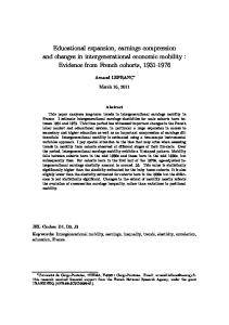
The last few decades have witnessed pronounced changes in relative average wages across groups of workers with different observable characteristics (between-group inequality). Most notably, the wages of workers with more education relative to those with less and of women relative to men have increased substantially in the United States. A large literature has emerged studying how changes in relative supply and demand for labor groups shape their relative wages. Changes in relative demand across labor groups have been linked prominently to computerization (or a reduction in the price of equipment more generally)—see e.g. Krusell et al. (2000), Autor and Dorn (2013), and Beaudry and Lewis (2014)—and to changes in relative demand across occupations and sectors, driven by structural transformation, offshoring, and international trade—see e.g. Autor et al. (2003), Buera et al. (2015), and Galle et al. (2015). Consistent with the first hypothesis, Table 1 shows that computer use rose dramatically between 1984 and 2003 and that computers are used more intensively by educated workers and women. Consistent with the second hypothesis, Figure 1 shows that education- and female-intensive occupations grew relatively quickly over the same time period.1

All Gender Education

Female Male College degree No college degree

1984

1989

1993

1997

2003

27.4 32.8 23.6 45.5 22.1

40.1 47.6 34.5 62.5 32.7

49.8 57.3 43.9 73.4 41.0

53.3 61.3 47.0 79.8 43.7

57.8 65.1 52.1 85.7 45.3

Table 1: Share of hours worked with computers We contribute to this literature by providing a unifying framework to simultaneously quantify these different determinants of between-group inequality. We use the model together with detailed data on factor allocations to assess the impact of computerization and changes in occupation demand on between-group inequality in the United States. We additionally quantify the extent to which computerization and changes in occupation demand are driven by international trade in equipment goods and occupation output. We base our analysis on an assignment model with many groups of workers and many occupations—building on Lagakos and Waugh (2013) and Hsieh et al. (2016)—which we extend to incorporate many types of equipment (such as computers) and international trade in occupation services and equipment goods. This framework allows for potentially 1 We

describe our data sources in depth in Section 4.1 and Appendix B.

1

Figure 1: Growth (1984-2003) of the occupation share of labor payments and the average (1984 & 2003) of the share of workers in the occupation who have a college degree (left) and are female (right) rich patterns of complementarity between computers, labor groups and occupations and, in spite of its high dimensionality, remains tractable enough to perform aggregate counterfactuals in a parsimonious manner. The model’s aggregate implications for relative wages nest those of workhorse models of between-group inequality in a closed economy, e.g. Katz and Murphy (1992) and Krusell et al. (2000), and in an open economy, e.g. Heckscher-Ohlin. In our model, the impact of changes in the economic environment on between-group inequality in a given country is shaped by comparative advantage between labor groups, equipment types, and occupations in that country, and comparative advantage across countries in different equipment types and occupations. Consider, for example, the potential impact of computerization, modeled as a reduction in the relative price of computers (driven by e.g. an increase in productivity of computers or a reduction in trade costs) on the relative wage of a labor group—such as educated workers or women—that uses computers intensively. A labor group may use computers intensively for two reasons. First, it may have a comparative advantage with computers, in which case this group would use computers relatively more within occupations, as is the case for more educated workers in the US. Our model predicts that a reduction in the price of computers increases the relative wage of this labor group. Second, a labor group may have a comparative advantage in occupations in which computers have a comparative advantage, in which case this group would be allocated disproportionately to occupations in which all workers are relatively more likely to use computers, as is the case for women in the US. Our model predicts that a reduction in the price of computers may increase or decrease the relative wage of this group depending on the degree of substitutability between occupations. We use our model to conduct two types of quantitative exercise. First, in a closed econ2

omy version of the model in which equipment prices and occupation demand shifters are taken as primitives, we conduct a decomposition of changes in relative wages between labor groups in the US between 1984 and 2003. Second, in an open economy extension of the model, we quantify the impact of international trade in equipment goods and occupation services on US relative wages in this time period, as well as the counterfactual impact that moving to autarky would have on US relative wages. For both of these exercises we must identify comparative advantage between US labor groups, equipment types, and occupations, estimate the elasticity of substitution between occupations, and estimate an elasticity shaping the within-worker dispersion of productivity across occupation-equipment type pairs. Comparative advantage can be inferred directly from data on the allocation of workers to equipment type-occupation pairs. In order to estimate the two key elasticities, we derive moment conditions that are consistent with equilibrium relationships generated by our model. To conduct the decomposition exercise, we also must measure computerization as well as changes in occupation demand, labor supply, and labor productivity in the US for the period 1984 to 2003. Changes in equipment productivity that result in computerization can be inferred from changes in the allocation of workers to computers within labor group-occupation pairs; focusing on changes within labor group-occupation pairs is important because aggregate computer usage will rise even in the absence of changes in equipment productivity if either labor groups that have a comparative advantage using computers or occupations that have a comparative advantage with computers grow. Occupation demand shifters can be inferred from changes in the allocation of workers to occupations within labor group-equipment type pairs and in labor income shares across occupations. Changes in labor composition are directly observed in the data. Finally, we measure labor productivity as a residual to match changes in the average wage of each labor group. As is evident from the previous discussion, our procedure crucially requires information for multiple years on the shares of workers of each labor group allocated to each equipment type-occupation pair. We obtain this information for the US from the October Current Population Survey (CPS) Computer Use Supplement, which provides data for five years (1984, 1989, 1993, 1999, and 2003) on whether a worker has direct or hands on use of a computer at work—be it a personal computer, laptop, mini computer, or mainframe—and on worker characteristics, hours worked, and occupation. For our purposes, this data is not without limitations: it imposes a narrow view of computerization that does not capture, e.g., automation of assembly lines; it only provides information on the allocation of workers to one type of equipment, computers; it does not detail the share of 3

each worker’s time at work spent using computers; and it only covers the period 19842003.2 In our decomposition exercise, our model predicts that computerization alone accounts for roughly 60% of all shocks that have had a positive impact on the skill premium (i.e. the relative wage of workers with a college degree to those without) between 1984 and 2003 and plays a similar role in explaining disaggregated measures of betweeneducation-group inequality (e.g., the wage of workers with graduate training relative to the average wage). Our model’s prediction is driven by the following three facts observed in the data. First, there has been a large rise in the share of workers using computers within labor group-occupation pairs, which our model interprets as a large increase in computer productivity (i.e. computerization). Second, more educated workers use computers within occupations relatively more than less educated workers, which our model interprets as educated workers having a comparative advantage with computers. This pattern of comparative advantage, together with computerization, yields a rise in the relative wages of educated workers according to our model. Third, more educated workers are also disproportionately employed in occupations in which all workers use computers relatively intensively. This pattern of sorting across occupations, together with computerization and an estimated elasticity of substitution between occupations greater than one, also yields a rise in the relative wages of educated workers according to our model. The combination of computerization and occupation shifters accounts for roughly 80% of the rise in the skill premium, leaving only 20% to be explained by labor productivity. This is remarkable, given that we measure changes in labor productivity as a residual that allows our framework to exactly match observed changes in relative wages. We find that computerization, occupation shifters, and labor productivity all play important roles in accounting for the reduction in the gender gap (i.e. the relative wage of male to female workers). Computerization decreases the gender gap because women are disproportionately employed in occupations in which all workers use computers intensively and our estimate of the elasticity of substitution across occupations is larger than one. Whereas in our closed economy model we treat computerization and changes in occupation demand as primitives, in sections 5 and 6 we study the extent to which these changes are a consequence of international trade. Theoretically, we show that the procedure to quantify the impact on relative wages of moving to autarky in equipment and 2 The

period 1984-2003, however, accounts for a substantial share of the increase in the skill premium and reduction in the gender gap observed in the US since the late 1960s. In Appendix F, we show that the German Qualification and Working Conditions survey, which alleviates some of the limitations of the CPS data, reveals similar patterns of comparative advantage in Germany as what the CPS data reveals for the US.

4

occupation trade is equivalent to the procedure we follow in our closed economy model to calculate the impact of domestic shocks on relative wages, with the only difference that the computerization and occupation demand shocks are now measured as functions of import shares of absorption and export shares of output of different equipment types and occupations. For example, if occupation ω has a high import share relative to occupation ω 0 , then moving to autarky has an equivalent impact on relative wages in a closed economy as increasing domestic occupation demand for ω relative to ω 0 . Given the lack of data on the occupation content of exports and imports, measuring occupation trade shares is a challenge; for a full discussion of the difficulties, see Grossman and Rossi-Hansberg (2007). Given these challenges, we consider alternative simple, albeit imperfect, approaches to measure the occupation content of exports and imports. Using our preferred approach, we find that moving from 2003 trade shares to equipment (occupation) autarky would generate a 2.2 (6.5) percentage point reduction in the skill premium. We also provide a simple procedure to quantify the differential effects on wages in a given country of changes in primitives (i.e. worldwide technologies, labor compositions, and trade costs) between two time periods relative to the effects of the same changes in primitives if that country were a closed economy. Using this latter result, we quantify the impact of trade in equipment goods and occupation services on between-group inequality in the US between 1984 and 2003. We find that equipment (occupation) trade accounts for roughly 13 percent (27 percent) of the rise in the skill premium between 1984 and 2003 accounted for by changes in equipment productivity (occupation demand) in our closed economy calculations. Our paper is organized as follows. In Section 2, we discuss the related literature. We describe our closed economy framework, characterize its equilibrium, and discuss its mechanisms in Section 3. We parameterize the model and present our closed economy results in Section 4. We extend our model to incorporate international trade in equipment goods and occupation services in Section 5 and quantify the impact of international trade in Section 6 . We conclude in Section 7. Additional details and robustness exercises are relegated to appendices.

2

Literature

We follow Lagakos and Waugh (2013) and Hsieh et al. (2016) in using a Roy (1951) model of the labor market parameterized with a Fréchet distribution. We extend previous versions of this model by introducing equipment types as another dimension along which workers sort, and international trade as another set of forces determining the equilibrium 5

assignment of workers to occupations and equipment types. This crucially allows us to study within a unified framework the impact of occupation demand shifters, computer productivity, labor productivity, labor composition, and trade costs on relative average wages of multiple groups of workers, such as the decline in the gender gap and the rise in the skill premium.3 In trying to explain the evolution of between-group inequality as a function of changes in observables, our paper’s objective is most similar to Krusell et al. (2000) and Lee and Wolpin (2010). Krusell et al. (2000) estimate an aggregate production function that permits capital-skill complementarity and show that changes in aggregate stocks of equipment, skilled labor, and unskilled labor can account for much of the variation in the US skill premium. Whereas Krusell et al. (2000) identify the degree of capital-skill complementarity using aggregate time series data, our approach leverages information on the allocation of workers to computers and occupations and, consequently, yields parameter estimates shaping the degree of equipment-labor group complementarity that are robust to allowing for time trends in the relative productivity of each labor group; see Acemoglu (2002) for a discussion of the relevance of allowing for these time trends in this context. Our decomposition corroborates the findings in Krusell et al. (2000) and extends them by additionally considering the impact of equipment productivity growth on the gender gap and other measures of between-group inequality. Lee and Wolpin (2010) use a dynamic model of endogenous human capital accumulation and find that labor group productivity (also treated as a residual in their analysis) plays the central role in explaining changes in the skill premium. By considering a greater degree of disaggregation in occupations and labor groups, our results reduce the role of changes in the residual in shaping changes in the skill premium. On the other hand, in contrast to Lee and Wolpin (2010), we treat labor composition as exogenous.4 3 The

relative importance of between- and within-group inequality is an area of active research. Autor (2014) concludes: “In the US, for example, about two-thirds of the overall rise of earnings dispersion between 1980 and 2005 is proximately accounted for by the increased premium associated with schooling in general and postsecondary education in particular.” On the other hand, Helpman et al. (Forthcoming) conclude: “Residual wage inequality is at least as important as worker observables in explaining the overall level and growth of wage inequality in Brazil from 1986-1995.” 4 Extending our model to endogenize education and labor participation—maintaining a static environment—would give rise to the same equilibrium equations determining factor allocations and wages conditional on labor composition. Our measures of shocks—to occupation shifters, equipment productivity, and labor productivity—and our estimates of model parameters are therefore robust to extending our model to endogenize the supply of each labor group in a static environment. Through the lens of this model, our counterfactual results would be interpreted as the direct effect of shocks to occupation shifters, equipment productivity, and labor productivity on labor demand and wages, taking labor composition as given.. If we also wanted to take into consideration the accumulation of occupation-specific human capital as in, e.g., Kambourov and Manovskii (2009a) and Kambourov and Manovskii (2009b), we would have to include occupational experience as a worker characteristic when defining labor groups in the data (unfortunately,

6

In modeling international trade, we operationalize in a quantitative setting the theoretical insights of Costinot and Vogel (2010), Sampson (2014), and Costinot and Vogel (2015) regarding the impact of international trade on inequality in high-dimensional environments. We show that one can use a similar approach to that introduced by Dekle et al. (2008) in a single-factor trade model—i.e. replacing a large number of unknown parameters with observable allocations in an initial equilibrium—in a many-factor assignment model. In this respect, our paper is complementary to concurrent work quantifying the impact of international trade on between-group inequality; see e.g. Adao (2015), DixCarneiro and Kovak (2015), Galle et al. (2015), and Lee (2016). Relative to this concurrent work, we introduce equipment in the framework and quantify the impact of trade both in equipment and in occupations on inequality; however, relative to this work we only use data for one region: the US. Whereas a large literature has emerged to argue that trade in occupation (or even task) output is a potentially important force generating changes in inequality—see e.g. Grossman and Rossi-Hansberg (2008)—there has been much less work conducting model-based counterfactuals to quantify the importance of this phenomenon.5 Given the crudeness of our measures of occupation trade, our quantification of the impact of trade in occupations should be viewed as a first step rather than the final word. Our modeling of international trade in equipment extends the quantitative analyses of Burstein et al. (2013) and Parro (2013), who study the impact of trade in capital equipment on the skill premium using the model of Krusell et al. (2000). Two related papers use differences in regional exposure to computerization to study the differential effect across regions of technical change on the polarization of US employment and wages, Autor and Dorn (2013), and on the gender gap and skill premium, Beaudry and Lewis (2014). Our approach complements these papers, embedding computerization into a general equilibrium model that allows us to quantify by means of counterfactual exercises the effect of computerization (as well as other shocks) on changes in between-group inequality.6 the October CPS does not contain this information) and model the corresponding dynamic optimization problem that workers would solve when deciding which occupation to sort into. 5 Traiberman (2016) quantifies the impact of import competition on occupation demand and wages. He constructs a measure of import exposure by occupation by allocating observed sectoral imports to occupations according to the share of labor payments going to each occupation in each industry. As we argue below, this measure is likely to be biased if, within industries, certain occupations are more traded than others. Instead of studying inequality, Goos et al. (2014) measure the impact of offshoring on the growth of occupations using data from sixteen European countries imposing a common effect of occupation offshorability on changes in occupation size independently of whether a country is a net exporter or a net importer in this occupation. Our model (analogous to the Heckscher-Ohlin model) emphasizes the importance of accounting for differences across countries in comparative advantage and, hence, distinguishing whether a country is a net exporter or importer of each occupation 6 Firpo et al. (2011) uses a statistical model of wage setting to investigate the contribution of changes

7

The approach that we use to bring our model to the data does not require mapping occupations into observable characteristics such as those introduced in Autor et al. (2003). Instead, we estimate measures of comparative advantage and occupation-specific demand shocks that vary flexibly across occupations, independently of the similarity in the task composition of these occupations. Even though the information on the task composition of occupations is never used in our analysis, we show in Appendix H.1 that changes in the size of occupations are not driven only by occupation demand shifters. For example, computerization generates an expansion in those occupations that happen to be intensive in non-routine cognitive analytical and interpersonal tasks and a contraction in occupations that are intensive in non-routine manual physical tasks. In exploiting data on workers’ computer usage, our paper is related to an earlier literature studying the impact of computer use on wages; see e.g. Krueger (1993) and Entorf et al. (1999). This literature identifies the impact of computer usage on wages by regressing wages of different workers on a dummy for computer usage, an identification approach that DiNardo and Pischke (1997) criticize. Our approach to estimate key model parameters does not rely on such a regression. We rely instead on an estimating equation first suggested by Acemoglu and Autor (2011) as an example of how their assignment model might be brought to the data.

3

Closed economy model

In this section we introduce the closed economy version of our model, characterize its equilibrium, and provide intuition for how different changes in the economic environment affect relative wages.

3.1

Environment

At time t there is a continuum of workers indexed by z ∈ Zt , each of whom inelastically supplies one unit of labor. We divide workers into a finite number of labor groups, indexed by λ. The set of workers in group λ is given by Zt (λ) ⊆ Zt , which has mass Lt (λ). There is a finite number of equipment types, indexed by κ. Workers and equipment are employed by production units to produce a finite number of occupations, indexed by ω.

in the returns to occupational tasks relative to changes in unionization and labor market wide returns to skills. Our paper complements theirs by incorporating general equilibrium effects and explicitly modeling the endogenous allocation of factors.

8

A final good is produced combining the services of occupations according to a constant elasticity of substitution (CES) production function

Yt =

∑ µt (ω )

!ρ/(ρ−1) 1/ρ

Yt (ω )

(ρ−1)/ρ

,

(1)

ω

where ρ > 0 is the elasticity of substitution across occupations, Yt (ω ) ≥ 0 is the endogenous output of occupation ω, and µt (ω ) ≥ 0 is an exogenous demand shifter for occupation ω.7 The final good is used to produce consumption, Ct , and equipment, Yt (κ ), according to the resource constraint Yt = Ct + ∑ p˜ t (κ ) Yt (κ ) ,

(2)

κ

where p˜ t (κ ) denotes the cost of a unit of equipment κ in terms of units of the final good.8 Occupation services are produced by perfectly competitive production units. A unit hiring k units of equipment type κ and l efficiency units of labor group λ produces kα [ Tt (λ, κ, ω ) l ]1−α units of output, where α denotes the output elasticity of equipment in each occupation and Tt (λ, κ, ω ) denotes the productivity of an efficiency unit of group λ’s labor in occupation ω when using equipment κ.9 Comparative advantage between labor and equipment is defined as follows: λ0 has a comparative advantage (relative to λ) using equipment κ 0 (relative to κ) in occupation ω if Tt (λ0 , κ 0 , ω )/Tt (λ0 , κ, ω ) ≥ Tt (λ, κ 0 , ω )/Tt (λ, κ, ω ). Labor-occupation and equipment-occupation comparative advantage are defined symmetrically. A worker z ∈ Zt (λ) supplies e (z) × ε (z, κ, ω ) efficiency units of labor if teamed with equipment κ in occupation ω. Each worker is associated with a unique e (z), allowing 7 We

show in Sections 5 and 6 that changes in the extent of international trade in occupation services generate endogenous changes in occupation demand shifters, µt (ω ). 8 We show in sections 5 and 6 how changes in the extent of international trade in equipment generate endogenous changes in equipment prices p˜ t (κ ). Our assumption that equipment must be produced every period (five-years in our quantitative analysis) is equivalent to assuming that equipment fully depreciates every period. Alternatively, we could have assumed that Yt (κ ) denotes investment in capital equipment κ, which depreciates at a given finite rate. All our counterfactual exercises are consistent with this alternative model with capital accumulation: they would correspond to comparisons across balanced growth paths in which the real interest rate and the growth rate of relative productivity across equipment types are constant over time. 9 We can extend the model to incorporate other inputs such as structure or intermediate inputs s; however, they would not affect any of our results as long asthey are produced linearly using the final good and  η

enter the production function multiplicatively as s1−η kα [ Tt (λ, κ, ω ) l ]1−α . Notice that, in either case, α is the share of equipment relative to the combination of equipment and labor. We restrict α to be common across ω because we do not have the data to estimate a different value of α(ω ) to each ω.

9

some workers within Zt (λ) to be more productive than others across all possible (κ, ω ); we normalize the average value of e (z) across workers within each λ to be one and prove this is without loss of generality in Appendix A. Each worker is also associated with a vector of ε (z, κ, ω ), one for each (κ, ω ) pair, allowing workers within Zt (λ) to vary in their relative productivities across (κ, ω ) pairs. We impose two restrictions. First, the distribution of e (z) has finite support and is independent of the distribution of ε (z, κ, ω ) for each (κ, ω ). Second, each ε (z, κ, ω ) is drawn independently from a Fréchet distribu
tion with cumulative distribution function G (ε) = exp ε−θ , where a higher value of θ > 1 implies lower within-worker dispersion of efficiency units across (κ, ω ) pairs.10 The assumption that ε (z, κ, ω ) is distributed Fréchet is made for analytical tractability; it implies that the average wage of a labor group is a CES function of occupation prices and equipment productivity.11 Total output of occupation ω, Yt (ω ), is the sum of output across all units producing occupation ω. All markets are perfectly competitive and all factors are freely mobile across occupations and equipment types. Relation to alternative frameworks. Whereas our framework imposes strong restrictions on occupation production functions, its aggregate implications for wages nest those in Katz and Murphy (1992) and Krusell et al. (2000). Specifically, the aggregate implications of our model for relative wages are equivalent to those in Katz and Murphy (1992) if we assume no equipment (i.e. α = 0) and two labor groups, each of which has a positive productivity in only one occupation. Similarly, the aggregate implications of our model for relative wages are equivalent to those in Krusell et al. (2000) if we allow for only two labor groups and one type of equipment, each labor group has positive productivity in only one occupation and the equipment share is positive in only one occupation.

3.2

Equilibrium

We characterize the competitive equilibrium, first taking occupation prices as given and then in general equilibrium. Additional derivations are provided in Appendix A. Partial equilibrium. With perfect competition, equation (2) implies that the price of equipment κ is simply pt (κ ) = p˜ t (κ ) Pt , where Pt is the price of the final good, which 10 See Adao (2015) for an approach that relaxes these two restrictions in an environment in which each worker faces exactly two choices. In Appendix G we show that our results are robust to allowing for specific forms of statistical dependence of ε (z, κ, ω ) across (κ, ω ) pairs. Moreover, we also conduct our analysis allowing for variation across labor groups in the dispersion parameter θ and show that our quantitative results are robust. 11 The wage distribution implied by this assumption is a good approximation to the observed distribution of individual wages; see e.g. Saez (2001) and Figure 3 in Appendix D.4.

10

we normalize to one so that pt (κ ) = p˜ t (κ ). An occupation production unit hiring k units of equipment κ and l efficiency units of labor λ earns revenues pt (ω ) kα [ Tt (λ, κ, ω ) l ]1−α and incurs costs pt (κ ) k + vt (λ, κ, ω ) l, where vt (λ, κ, ω ) is the wage per efficiency unit of labor λ when teamed with equipment κ in occupation ω and pt (ω ) is the price of occupation ω output. The profit maximizing choice of equipment quantity and the zero profit condition—due to costless entry of production units—yield −α

1

vt (λ, κ, ω ) = α¯ pt (κ ) 1−α pt (ω ) 1−α Tt (λ, κ, ω ) if there is positive entry in (λ, κ, ω ), where α¯ ≡ (1 − α) αα/(1−α) . Facing the wage profile vt (λ, κ, ω ), each worker z ∈ Zt (λ) chooses the equipment-occupation pair (κ, ω ) that maximizes her wage, e (z) ε (z, κ, ω ) vt (λ, κ, ω ). The assumption that ε (z, κ, ω ) is distributed Fréchet and independent of e (z) implies that the probability that a randomly sampled worker, z ∈ Zt (λ), uses equipment κ in occupation ω is iθ −α 1 Tt (λ, κ, ω ) pt (κ ) 1−α pt (ω ) 1−α πt (λ, κ, ω ) = h iθ . −α 1 0 0 0 0 ∑κ 0 ,ω 0 Tt (λ, κ , ω ) pt (κ ) 1−α pt (ω ) 1−α h

(3)

The higher is θ—i.e. the less dispersed are efficiency units across (κ, ω ) pairs—the more responsive are factor allocations to changes in prices or productivities. According to equation (3), comparative advantage shapes factor allocations. As an example, the assignment of workers across equipment types within any given occupation satisfies Tt (λ0 , κ 0 , ω ) Tt (λ0 , κ, ω )



Tt (λ, κ 0 , ω ) = Tt (λ, κ, ω )



πt (λ0 , κ 0 , ω ) πt (λ0 , κ, ω )



πt (λ, κ 0 , ω ) πt (λ, κ, ω )

1/θ ,

so that, if λ0 workers (relative to λ) have a comparative advantage using κ 0 (relative to κ) in occupation ω, then they are relatively more likely to be allocated to κ 0 in occupation ω. The wage per efficiency unit of labor λ when teamed with equipment κ in occupation ω, vt (λ, κ, ω ), differs from the average wage of workers in group λ teamed with equipment κ in occupation ω, denoted by wt (λ, κ, ω ), which is the integral of e (z) ε (z, κ, ω ) vt (λ, κ, ω ) across workers teamed with κ in occupation ω, divided by the mass of these workers. Given our assumptions on e (z) and ε (z, κ, ω ), we obtain −α

1

wt (λ, κ, ω ) = α¯ γTt (λ, κ, ω ) pt (κ ) 1−α pt (ω ) 1−α πt (λ, κ, ω )−1/θ , where γ ≡ Γ (1 − 1/θ ) and Γ (·) is the Gamma function. An increase in productivity 11

or occupation price, Tt (λ, κ, ω ) or pt (ω ), or a decrease in equipment price, pt (κ ), raises the wages of infra-marginal λ workers allocated to (κ, ω ). However, the average wage across all λ workers in (κ, ω ) increases less than that of infra-marginal workers due to self-selection, i.e. πt (λ, κ, ω ) increases, which lowers the average efficiency units of the λ workers who choose to use equipment κ in occupation ω. Denoting by wt (λ) the average wage of workers in group λ (i.e. total income of the workers in group λ divided by their mass), the previous expression and equation (3) imply wt (λ) = wt (λ, κ, ω ) for all (κ, ω ), where12

wt (λ) = α¯ γ

∑



Tt (λ, κ, ω ) pt (κ )

−α 1− α

pt (ω )

1 1− α

θ

!1/θ .

(4)

κ,ω

General equilibrium. In any period, occupation prices pt (ω ) must be such that total expenditure in occupation ω is equal to total revenue earned by all factors employed in occupation ω, 1 ζ t (ω ) , (5) µt (ω ) pt (ω )1−ρ Et = 1−α where Et ≡ (1 − α)−1 ∑λ wt (λ) Lt (λ) is total expenditure (which equals total income in a closed economy) and ζ t (ω ) ≡ ∑λ,κ wt (λ) Lt (λ) πt (λ, κ, ω ) is total labor income in occupation ω. The left-hand side of equation (5) is expenditure on occupation ω and the right-hand side is total income earned by factors employed in occupation ω. In equilibrium, the aggregate quantity of the final good is such that Yt = Et , the aggregate quantity of equipment κ is Yt (κ ) =

α 1 ∑ πt (λ, κ, ω ) wt (λ) Lt (λ) , pt (κ ) 1 − α λ,ω

and aggregate consumption is determined by equation (2).

3.3

System in changes

To solve for changes in wages in response to changes in the economic environment, we express the system of equilibrium equations described in Section 3.2 in changes, denoting 12 The

implication that average wage levels are common across occupations within λ (which is inconsistent with the data) obviously implies that the changes in wages will also be common across occupations within λ. In Appendix I we decompose the observed changes in average wages for each λ into a between occupation component (which is zero in our model) and a within occupation component and show that the between component is small. Furthermore, we show that by incorporating preference shifters for working in different occupations that generate compensating differentials, similar to Heckman and Sedlacek (1985), our model can generate differences in average wage levels across occupations within a labor group.

12

changes in any variable x between any two periods t0 and t1 by xˆ ≡ xt1 /xt0 . Changes in average wages are given by

wˆ (λ) =

∑



Tˆ (λ, κ, ω ) pˆ (κ )

−α 1− α

pˆ (ω )

1 1− α

θ

!1/θ πto (λ, κ, ω )

(6)

κ,ω

and changes in occupation prices are determined by the following system of equations iθ 1 −α ˆ 1 − α 1 − α T (λ, κ, ω ) pˆ (κ ) pˆ (ω ) πˆ (λ, κ, ω ) = h iθ −α 1 0 0 0 0 ˆ 1 − α 1 − α ˆ ˆ πt0 (λ, κ 0 , ω 0 ) ∑κ 0 ,ω 0 T (λ, κ , ω ) p (κ ) p (ω ) h

µˆ (ω ) pˆ (ω )1−ρ Eˆ =

1 wt0 (λ) Lt0 (λ) πt0 (λ, κ, ω ) wˆ (λ) Lˆ (λ)πˆ (λ, κ, ω ), ζ t0 ( ω ) ∑ λ,κ

(7)

(8)

wt ( λ ) Lt ( λ ) and where Eˆ = ∑λ (01−α)E0 wˆ (λ) Lˆ (λ). In this system, the forcing variables are: Lˆ (λ), t0 Tˆ (λ, κ, ω ), µˆ (ω ), and pˆ (κ ). Given these variables, equations (6)-(8) yield the model’s

implied values of changes in average wages, wˆ (λ), allocations, πˆ (λ, κ, ω ), occupation ˆ prices, pˆ (ω ), and total expenditure, E.

3.4

Intuition

The impact of shocks on wages. According to equation equation (6), changes in productivities Tˆ (λ, κ, ω ) and in the price of equipment pˆ (κ ) have a direct effect (i.e. holding occupation prices constant) on wages. In addition, both these shocks as well as changes in occupation shifters and in labor composition affect wages indirectly through their impact on equilibrium occupation prices pˆ (ω ). The importance of changes in productivities, equipment prices, and occupation prices for changes in group λ’s average wage depends on factor allocations in the initial period, πt0 (λ, κ, ω ). For example, an increase in occupation ω’s price or a reduction in the price of equipment κ between t0 and t1 raises the relative average wage of labor groups that disproportionately work in occupation ω or use equipment κ in period t0 . We now discuss in more detail the intuition for the impact of each of the shocks (the forcing variables) we consider in our quantitative analysis below. Consider an increase in the occupation demand, i.e. µˆ (ω ) > 1. This shock raises the price of occupation ω and, therefore, the relative wage of labor groups that are disproportionately employed in occupation ω. Similarly, a decrease in labor supply, i.e. Lˆ (λ) < 1, raises the relative price of occupations in which group λ is disproportionately employed. This raises the relative 13

wage not only of group λ, but also of other labor groups employed in similar occupations as λ.13 A proportional increase across all (κ, ω ) in labor productivity for group λ—i.e. Tˆ (λ, κ, ω ) = Tˆ (λ) > 1—directly raises the relative wage of group λ and reduces the relative price of occupations in which this group is disproportionately employed, thus reducing the relative wage of labor groups employed in similar occupations as λ.14 Consider the impact of a decrease in the price of equipment κ, i.e. pˆ (κ ) < 1, or a proportional increase in its productivity across all (λ, ω ), i.e. Tˆ (λ, κ, ω ) = Tˆ (κ ) > 1. The impact of these two shocks being equivalent, we focus on a reduction in the price of equipment κ for illustration purposes. The partial equilibrium impact of this shock is to raise the relative wage of labor groups that use κ intensively. In general equilibrium this shock also reduces the relative price of occupations in which κ is used intensively, lowering the relative wage of labor groups that are disproportionately employed in these occupations. Overall, the impact on relative wages of changes in equipment price depends on the value of ρ and on whether aggregate patterns of labor allocation across equipment types are mostly a consequence of variation in labor-equipment comparative advantage or mainly determined by variation in labor-occupation and equipment-occupation comparative advantage. Let us consider two extreme cases. If the only form of comparative advantage is between workers and equipment, then a decrease in the price of κ does not affect relative occupation prices (since all occupations are equally intensive in κ) and, therefore, the effect conditional on maintaining fixed occupation prices is the same as the general equilibrium effect: a decrease in the price of κ will increase the relative wages of worker groups that use equipment κ more intensively in the initial period. If there is no comparative advantage between workers and equipment but there is comparative advantage between workers and occupations and between equipment and occupations, then a decrease in the price of κ has two opposite effects on the relative wages of worker groups that use equipment κ intensively; i.e. those disproportionately employed in κ-intensive occupations. While it has a positive effect conditional on occupation prices, it has a negative effect indirectly through its effect on occupation prices. The relative strength of the direct and indirect channels depends on ρ. The direct effect dominates if and only if ρ > 1. Intuitively, a decrease in the price of κ acts like a pos13 In Appendix D.5 we provide empirical evidence that supports our model’s implication that changes in labor composition affect wages only indirectly through occupation prices. 14 Costinot and Vogel (2010) provide analytic results on the implications for relative wages of changes in labor composition, Lt (λ), and occupation demand, µt (ω ), in a restricted version of our model in which there are no differences in efficiency units across workers in the same labor group (i.e. θ = ∞), there is no capital equipment (i.e. α = 0), and T (λ, ω )—i.e. our T (λ, κ, ω ) in the absence of equipment—is logsupermodular.

14

itive productivity shock to the occupations in which κ has a comparative advantage. If ρ > 1, this increases employment and the relative wages of labor groups disproportionately employed in the occupations in which κ has a comparative advantage. The opposite is true if ρ < 1. In our framework computerization can hence either contract or expand employment in occupations that are computer intensive. More generally—outside of these two extreme cases—a decrease in the price of computers can simultaneously raise the wage (relative to the average wage) of one labor group (λ1 ) that uses computers intensively while reducing the wage (relative to the average wage) of another labor group (λ2 ) that uses computers intensively. This would be the case if λ1 has a comparative advantage using computers, λ2 has a comparative advantage in the occupations in which computers have a comparative advantage, and ρ < 1. The role of θ and ρ. The parameter θ, which governs the degree of within-worker dispersion of productivity across occupation-equipment type pairs, determines the extent of worker reallocation in response to changes in occupation prices, equipment prices, and productivities: a higher dispersion of idiosyncratic draws, as given by a lower value of θ, results in less worker reallocation. In order to gain intuition on the role of θ for changes in labor group average wages, we take a first-order approximation of equation (6) at period t0 allocations: 

log wˆ (λ) = ∑ πt0 (λ, κ, ω ) log Tˆ (λ, κ, ω ) + κ,ω

 α 1 log pˆ (ω ) − log pˆ (κ ) . 1−α 1−α

(9)

This expression shows that, given changes in occupation and equipment prices as well as productivities, the change in average wages does not depend on θ up to a first-order approximation.15 However, a lower value of θ results in less worker reallocation across occupations in response to a shock and, therefore, larger changes in occupation prices. Hence, to a first-order approximation, the value of θ affects the response of average wages to shocks by affecting occupation price changes. The parameter ρ determines the elasticity of substitution between occupations, with a higher value of ρ reducing the responsiveness of occupation prices to shocks and hence, reducing the impact through occupation price changes of shocks on relative wages. For example, because labor composition only affects relative wages through occupation prices, a higher value of ρ reduces the impact of changes in labor composition on relative wages. Similarly, as described above, a higher value of ρ reduces the negative effects of comput15 More

generally, given changes in occupation prices, the shape of the distribution of ε (z, κ, ω )—which we have assumed to be Fréchet—does not matter for the first-order effect of any shock on average wage changes. The reason is that, for any worker group λ, the marginal worker’s wage is equal across occupations and equipment types.

15

erization on wages of labor groups with a comparative advantage on occupations that use computers intensively.

4

Decomposition

In this section we use our closed economy model to quantify the impact of computerization, changes in labor composition, changes in occupation demand, and changes in a labor-group specific productivity on observed changes in relative wages in the US. Throughout this section we assume that Tt (λ, κ, ω ) can be expressed as Tt (λ, κ, ω ) ≡ Tt (λ) Tt (κ ) Tt (ω ) T (λ, κ, ω ).

(10)

Accordingly, whereas we allow labor group, Tt (λ), equipment type, Tt (κ ), and occupation, Tt (ω ), productivity to vary over time, we impose that the interaction between labor group, equipment type, and occupation productivity, T (λ, κ, ω ), is constant over time. We therefore assume that comparative advantage is fixed over time. This restriction allows us to separate cleanly the impact on relative wages of λ-, κ-, and ω-specific productivity shocks.16 Given restriction (10), the system in changes given in equations (6)-(8) simplifies to " wˆ (λ) = Tˆ (λ)

∑ (qˆ (ω )qˆ (κ ))θ πt0 (λ, κ, ω )

#1/θ (11)

κ,ω

(qˆ (ω )qˆ (κ ))θ πˆ (λ, κ, ω ) = θ ∑κ 0 ,ω 0 (qˆ (ω 0 )qˆ (κ 0 )) πt0 (λ, κ 0 , ω 0 ) aˆ (ω )qˆ (ω )(1−α)(1−ρ) Eˆ =

∑λ,κ wt0 (λ) Lt0 (λ) πt0 (λ, κ, ω ) wˆ (λ) Lˆ (λ)πˆ (λ, κ, ω ) . ζ t0 ( ω )

(12)

(13)

In this simplified system, equipment productivity, Tt (κ ), is combined with equipment −α prices, pt (κ ), to form a composite equipment productivity measure: qt (κ ) ≡ pt (κ ) 1−α Tt (κ ). Similarly, occupation productivity, Tt (ω ), is combined with occupation demand, µt (ω ), to form a composite occupation shifter: at (ω ) ≡ µt (ω ) Tt (ω )(1−α)(ρ−1) . Finally, occupation productivity, Tt (ω ), is combined with occupation prices, pt (ω ), to form transformed occupation prices: qt (ω ) ≡ pt (ω )1/(1−α) Tt (ω ). In this system, the forcing variables (shocks) are: (i ) Lˆ (λ), which we refer to as labor composition; (ii ) qˆ (κ ), which we refer 16 Our results are robust when we perform a set of decompositions that relax this restriction in Appendix

E.3. We drop this restriction entirely when computing the international trade counterfactuals in Section 6.

16

to as equipment productivity; (iii ) aˆ (ω ), which we refer to as occupation shifters; and (iv) Tˆ (λ), which we refer to as labor productivity. Given these shocks, equations (11)-(13) yield the model’s implied values of changes in average wages, wˆ (λ), allocations, πˆ (λ, κ, ω ), ˆ 17 transformed occupation prices, qˆ (ω ), and total expenditure, E. According to equations (11)-(13), we need the following ingredients to perform our decomposition. First, we require measures of factor allocations, πt0 (λ, κ, ω ), average wages, wt0 (λ), labor composition, Lt0 (λ), and labor payments by occupation, ζ t0 (ω ). We describe the data we employ to obtain each of these measures in Section 4.1. Second, we require measures of relative shocks to labor composition, Lˆ (λ)/ Lˆ (λ1 ), occupation shifters, aˆ (ω )/ aˆ (ω1 ), equipment productivity to the power θ, qˆ(κ )θ /qˆ(κ1 )θ , and labor productivity, Tˆ (λ)/ Tˆ (λ1 ).18 We describe our approach to measure these shocks in Section 4.2. Finally, we require estimates of α, ρ, and θ. We describe our estimation strategy to assign values to these parameters in Section 4.3. Finally, we combine these ingredients and describe the results of our decomposition exercise in Section 4.4.

4.1

Data

We use data from the Combined CPS May, Outgoing Rotation Group (MORG CPS) and the October CPS Supplement (October Supplement) for the years 1984, 1989, 1993, 1997, and 2003. We restrict our sample by dropping workers who are younger than 17 years old, do not report positive paid hours worked, or are self employed. After cleaning, the MORG CPS and October Supplement contain data for roughly 115,000 and 50,000 individuals, respectively, in each year.19 We divide workers into thirty labor groups by gender, education (high school dropouts, high school graduates, some college completed, college completed, and graduate training), and age (17-30, 31-43, and 44 and older). We consider two types of equipment: computers and other equipment. We use thirty occupations, which we list, together with summary statistics, in Table 9 in Appendix B. 17 The

two components of equipment productivity, Tt (κ ) and pt (κ ), could be measured separately using information on equipment prices, which are subject to known quality-adjustment issues raised by, e.g., Gordon (1990). Similarly, the two components of the occupation shifter, Tt (ω ) and µt (ω ), could be measured separately using information on occupation prices, which are hard to measure in practice. If the aim of our exercise were not to determine the impact of observed changes in the economic environment on observed wages but rather to predict the impact of counterfactual or hypothetical changes in the economic environment, then it would not be necessary to combine changes in equipment productivity and equipment production costs into a single shock or to combine changes in occupation demand and occupation productivity into a single composite shock. 18 In Appendix C we show formally that changes in relative wages can be expressed as functions of relative shocks and that Eˆ cancels from the resulting system of equations. 19 We provide additional details on the data in Appendix B.

17

We use the MORG CPS to construct total hours worked and average hourly wages by labor group by year.20 We use the October Supplement to construct the share of total hours worked by labor group λ that is spent using equipment type κ in occupation ω in year t, πt (λ, κ, ω ). In 1984, 1989, 1993, 1997, and 2003, the October Supplement asked respondents whether they “have direct or hands on use of computers at work,” “directly use a computer at work,” or “use a computer at/for his/her/your main job.” The question defines a computer as a machine with typewriter like keyboards, whether a personal computer, laptop, mini computer, or mainframe. Identifying computers with the index κ 0 and the other equipment with the index κ 00 , we construct πt (λ, κ 0 , ω ) as the hours worked in occupation ω by λ workers who report that they use a computer at work relative to the total hours worked by labor group λ in year t, and construct πt (λ, κ 00 , ω ) as the hours worked in occupation ω by λ workers who report that they do not use a computer at work relative to the total hours worked by labor group λ in year t.21 When interpreting our measures of factor allocations, πt (λ, κ, ω ), one should bear in mind four limitations. First, our view of computerization is narrow. Second, at the individual level our computer-use variable takes only two values: zero or one. Third, we are not using any information on the allocation of non-computer equipment. Finally, the computer use question was discontinued after 2003.22 Factor allocation. Aggregating πt (λ, κ, ω ) across ω and λ, Table 1 shows that women and more educated workers use computers more intensively in the aggregate than men and less educated workers, respectively. The disaggregated πt (λ, κ, ω ) data also allows us also to identify sorting patterns across labor groups that condition on occupation or equipment types. Specifically, to determine the extent to which college educated workers (λ0 ) compared to workers with high school degrees in the same gender-age group (λ) use 20 We measure wages using the MORG CPS rather than the March CPS. Both datasets imply similar changes in average wages for each of our thirty labor groups. However, the March CPS does not directly measure hourly wages of workers paid by the hour and, therefore, introduces substantial measurement error in individual wages, see Lemieux (2006). For most of our analysis, we do not use individual wages; however, we do so in sensitivity analyses in Appendix D.4. 21 On average across the five years considered in the analysis, we measure π ( λ, κ, ω ) = 0 for roughly t 27% of the (λ, κ, ω ) triplets. As a robustness check, in Appendix H.2 we drop age as a characteristic defining a labor group and redo our analysis with the resulting ten labor groups. With only ten labor groups, the share of measured allocations πt (λ, κ, ω ) that are equal to 0 is substantially smaller. Our results are largely robust to decreasing the number of labor groups from 30 to 10. 22 The German Qualification and Working Conditions survey, used in e.g. DiNardo and Pischke (1997), helps mitigate the second and third concerns by providing data on worker usage of multiple types of equipment and, in 2006, the share of hours spent using computers. In Appendix F, we show using this more detailed German data similar patterns of comparative advantage—between computers and education groups and between computers and gender—as in the US data. We do not compute our accounting exercise for Germany because wage data for German workers reported in publicly available datasets has been described as unreliable, see e.g. Dustmann et al. (2009).

18

computers (κ 0 ) relatively more than non-computer equipment (κ) within occupations (ω), the left panel of Figure 2 plots the histogram of

πt λ, κ 0 , ω πt λ0 , κ 0 , ω
− log
log πt λ0 , κ, ω πt λ, κ, ω across all five years, thirty occupations, and six gender-age groups described above. Figure 2 shows that college educated workers are relatively more likely to use computers within occupations compared to high school educated workers; hence, according to our model, college educated workers have a comparative advantage using computers within occupations relative to high school educated workers. A similar conclusion holds comparing across other education groups: more educated workers always have a comparative advantage using computers.

Figure 2: Computer relative to non-computer usage for college degree relative to high school degree workers (female relative to male workers) in the left (right) panel The right panel of Figure 2 plots a similar histogram, where λ0 and λ now denote female and male workers in the same education-age group. This figure shows that there is no clear difference on average in computer usage across genders within occupations (i.e. the histogram is roughly centered around zero). Hence, our model rationalizes the fact that women use computers more than men at the aggregate level—see Table 1—by concluding that women have a comparative advantage in occupations in which computers have a comparative advantage. For instance, we observe that women are much more likely than men to work in administrative support relative to construction occupations, conditional on the type of equipment used; and that computers are much more likely to be used in administrative support than in construction occupations, conditional on labor group. These comparisons provide an example of a more general relationship: women tend to be employed in occupations in which all labor groups are relatively more likely to use computers.

19

4.2

Measuring shocks

Here we describe our baseline procedure to measure the four shocks into which we decompose changes in relative average wages: labor composition, Lˆ (λ)/ Lˆ (λ1 ), equipment productivity (to the power θ), qˆ(κ )θ /qˆ(κ1 )θ , occupation shifters, aˆ (ω )/ aˆ (ω1 ), and labor productivity, Tˆ (λ)/ Tˆ (λ1 ). We measure changes in labor composition directly from the MORG CPS. We measure changes in equipment productivity using data only on changes in disaggregated factor allocations over time, πˆ (λ, κ, ω ). We measure changes in occupation shifters using data on changes in disaggregated factor allocations and labor income shares across occupations as well as model parameters. Finally, we measure changes in labor productivity as a residual to match observed changes in relative wages. We provide details on the baseline procedure described here in Appendix C.1 and alternative procedures in Appendices C.2 and C.3. All these procedures yield very similar results. First, consider the measurement of changes in equipment productivity to the power θ. Equation (12) implies πˆ (λ, κ, ω ) qˆ(κ )θ = (14) θ πˆ (λ, κ1 , ω ) qˆ(κ1 ) for any (λ, ω ) pair. Hence, if computer productivity rises relative to other equipment between t0 and t1 , then the share of λ hours spent working with computers relative to other equipment in occupation ω will increase. It is important to condition on (λ, ω ) pairs when identifying changes in equipment productivity because unconditional growth over time in computer usage, shown in Table 1, may also reflect growth in the supply of labor groups who have a comparative advantage using computers and/or changes in occupation shifters that are biased towards occupations in which computers have a comparative advantage. We combine these (λ, ω ) pair-specific measures to obtain a unique measure of changes in equipment productivity to the power θ, qˆ(κ )θ /qˆ(κ1 )θ , as described in Appendix C.1. Second, consider the measurement of changes in occupation shifters. Equation (13) implies   ζˆ(ω ) qˆ(ω ) (1−α)(ρ−1) aˆ (ω ) = . (15) aˆ (ω1 ) ζˆ(ω1 ) qˆ(ω1 ) We construct the right-hand side of equation (15) in two steps as follows. First, equation (12) implies qˆ(ω )θ πˆ (λ, κ, ω ) = (16) θ πˆ (λ, κ, ω1 ) qˆ(ω1 ) for any (λ, κ ) pair. We combine these (λ, κ ) pair-specific measures to obtain a unique

20

measure of changes in transformed occupation prices to the power θ, qˆ(ω )θ /qˆ(ω1 )θ , as described in Appendix C.1.23 Given values of α, ρ, and θ, we recover (qˆ(ω )/qˆ(ω1 ))(1−α)(ρ−1) . We describe how we estimate these three parameters below. Second, given values of qˆ(κ )θ /qˆ(κ1 )θ and qˆ(ω )θ /qˆ(ω1 )θ , we construct ζˆ(ω )/ζˆ(ω1 ) using the right-hand side of equation (13). Note that if ρ = 1, changes in occupation shifters depend only on changes in the share of labor payments across occupations. Finally, we measure changes in labor productivity as a residual to match changes in relative wages. Specifically, we rewrite equation (11) as Tˆ (λ) wˆ (λ) = wˆ (λ1 ) Tˆ (λ1 )



sˆ (λ) sˆ (λ1 )

1/θ ,

(17)

where sˆ (λ) is a labor-group-specific weighted average of changes in equipment productivity and transformed occupation prices, both raised to the power θ, sˆ (λ) =

qˆ (ω )θ qˆ(κ )θ

∑ qˆ

κ,ω

(ω1 )θ qˆ (κ1 )θ

πt0 (λ, κ, ω ),

(18)

which we can construct using observed allocations, changes in observed allocations, and equations (14) and (16). Given wage data and a value of θ, we recover Tˆ (λ) / Tˆ (λ1 ). Note that only our measures of changes in labor productivities are directly a function of the observed changes in relative wages that we aim to decompose: given parameters α, ρ, and θ, observed changes in wages do not affect our measures of changes in labor composition or equipment productivity to the power θ, and they only affect our measures of occupation shifters indirectly through their impact on ζˆ(ω )/ζˆ(ω1 ).

4.3

Parameter estimates

The Cobb-Douglas parameter α, which matters for our results only when ρ is different from one, determines payments to all equipment (computers and non-computer equipment) relative to the sum of payments to equipment and labor. We set α = 0.24, consistent with estimates in Burstein et al. (2013). Burstein et al. (2013) disaggregate total capital payments (i.e the product of the capital stock and the rental rate) into structures and equipment using US data on the value of capital stocks and—since rental rates are not directly observable—setting the average rate of return over the period 1963-2000 of 23 We

use data on observed allocations to measure these changes in transformed occupation prices. In calculating changes in relative wages in response to any subset of shocks in our decomposition, we solve for counterfactual changes in transformed occupation prices and allocations using equations (12) and (13).

21

holding each type of capital (its rental rate plus price appreciation less the depreciation rate) equal to the real interest rate. As a reminder, the parameter θ determines the within-worker dispersion of productivity across occupation-equipment type pairs and the parameter ρ is the elasticity of substitution across occupations in the production of the final good. We estimate these two parameters jointly using a method of moments approach. In order to derive the relevant moment conditions, we rewrite equation (17) as log wˆ (λ, t) = ς θ (t) + (1/θ ) log sˆ (λ, t) + ι θ (λ, t) , (19) where sˆ (λ, t) is defined in equation (18), ς θ (t) ≡ log qˆ (ω1 , t) qˆ (κ1 , t) is a time effect that is common across λ, and ι θ (λ, t) ≡ log Tˆ (λ, t) captures unobserved changes in labor productivity.24 Similarly, equation (13) can be expressed as qˆ (ω, t)θ + ι ρ (ω, t) . log ζˆ (ω, t) = ς ρ (t) + ((1 − α) (1 − ρ) /θ ) log qˆ (ω1 , t)θ

(20)

where qˆ (ω, t)θ /qˆ (ω1 , t)θ is defined in equation (16), ς ρ (t) is a time effect that is common across ω and ι ρ (ω, t) ≡ log aˆ (ω, t) captures unobserved changes in occupation shifters. Equations (19) and (20) may be used to jointly identify θ and ρ. According to our model, however, the observed covariate in equation (19), log sˆ (λ, t), is predicted to be correlated with its error term, ι θ (λ, t), and the observed covariate in equation (20) is predicted to be correlated with its error term, ι ρ (ω, t). To address the endogeneity of these covariates, we construct instruments using different averages of observed changes in equipment productivity to the power θ, qˆ(κ, t)θ /qˆ(κ1 , t)θ . Specifically, we instrument the covariate log sˆ (λ, t) using a labor-group-specific average, log ∑ κ

qˆ(κ, t)θ qˆ(κ1 , t)θ

∑ π1984 (λ, κ, ω ), ω

and the covariate log qˆ(ω, t)θ /qˆ (ω1 , t)θ using an occupation-specific average log ∑ κ

qˆ(κ, t)θ qˆ(κ1 , t)θ

∑∑ λ

L1984 (λ) π1984 (λ, κ, ω ) . 0 0 0 λ0 ,κ 0 L1984 ( λ ) π1984 ( λ , κ , ω )

We use these two instruments and equations (19) and (20) to build moment conditions that identify the parameter vector (θ,ρ).25 24 For the purposes of this section, for any variable x, we use xˆ ( t ) to denote the relative change in a variable x between any two periods t and t0 > t. 25 Additional details on these moment conditions are provided in Appendix D. This appendix also contains a detailed discussion of how, under the assumptions of our model, these two instruments are valid

22

Our estimates exploit data on four time periods: 1984-1989, 1989-1993, 1993-1997, and 1997-2003. We report the point estimates and standard errors in the top row of Table 2. The resulting estimate of θ is 1.78 with a standard error of 0.29; the estimate of ρ is also 1.78 but with a slightly larger standard error of 0.35. In reviewing Krusell et al. (2000), Acemoglu (2002) raises a concern that may affect the estimates of θ and ρ computed using equations (19) and (20) as estimating equations. Specifically, they point out that the presence of common trends in unobserved labor-group-specific productivity, explanatory variables, and instruments may bias the estimates of wage elasticities. In order to address this concern, we follow Katz and Murphy (1992) and Acemoglu (2002) and additionally control for a λ-specific time trend in equation (19). In addition, we also control for an occupation-specific time trend in equation (20). The MM estimates of θ and ρ that result from adding as controls a labor-groupspecific time trend in equation (19) and an occupation-specific time trend in equation (20) are, respectively 1.13, with a standard error of 0.32, and 2, with a standard error of 0.71, as displayed in row 2 of Table 2.26 Parameter Time Trend? Estimate (SE) (θ, ρ) NO (1.78, 1.78) (0.29, 0.35) (θ, ρ) YES (1.13, 2.00) (0.32, 0.71) Table 2: Parameter estimates based on joint estimation When computing the main results of our analysis, we verify in Appendix E.1 the robustness of our conclusions to the different estimates of θ and ρ reported in this section and in Appendix D.

4.4

Results

In this section we summarize the results of our decomposition of observed changes in relative wages in the US between 1984 and 2003 into the contributions of changes in labor composition, occupation shifters, equipment productivity, and labor productivity. We construct various measures of changes in between-group inequality, each of them aggreand expected to be correlated with the corresponding endogenous variables. 26 In Appendix D we provide estimates of θ and ρ that rely on alternative identification assumptions. First, we report MM estimates that use versions of both equation (19) and equation (20) in levels instead of time differences; the resulting estimates are θ =1.57, with a standard error of 0.14, and ρ = 3.27, with a standard error of 1.34. Second, we follow Lagakos and Waugh (2013) and Hsieh et al. (2016) and identify θ from moments of the unconditional distribution of observed wages within each labor group λ; the resulting estimate of θ is equal to 2.62. Finally, we also estimate θ and ρ without instruments and show that the bias in each parameter is consistent with the predictions of our theory.

23

gating wage changes across our thirty labor groups in different ways (e.g., the skill premium). As is standard, when doing so, both in the model and in the data, we construct composition-adjusted wage changes; that is, for each aggregated measure we report, we average wage changes across the corresponding labor groups using constant weights over time, as described in detail in Appendix B. For each measure of inequality, we report its cumulative log change between 1984 and 2003, calculated as the sum of the log change over all sub-periods in our data.27 We also report the log change over each sub-period in our data. Skill premium. The first column in Table 3 reports the change observed in the data, which is also the change predicted by our model when all shocks—in labor composition, occupation shifters, equipment productivity, and labor productivity—are simultaneously considered. The skill premium increased by 15.1 log points between 1984 and 2003, with the largest increases occurring between 1984 and 1993. The subsequent four columns summarize the counterfactual change in the skill premium predicted by the model if only one of the four shocks is considered (i.e. holding the other exogenous parameters at their t0 level).

1984 - 1989 1989 - 1993 1993 - 1997 1997 - 2003 1984 - 2003

Data

Labor comp.

Occ. shifters

Equip. prod.

Labor prod.

0.057 0.064 0.037 -0.007 0.151

-0.031 -0.017 -0.023 -0.043 -0.114

0.026 -0.009 0.044 -0.011 0.049

0.052 0.045 0.021 0.042 0.159

0.009 0.046 -0.005 0.006 0.056

Table 3: Decomposing changes in the log skill premium (the wage of workers with a college degree relative to those without) Changes in labor composition decrease the skill premium in each sub-period. Specifically, the increase in hours worked by those with college degrees relative to those without of 47.4 log points between 1984 and 2003 decreases the skill premium by 11.4 log points. Changes in relative demand across labor groups must, therefore, compensate for the impact of changes in labor composition in order to generate the observed rise of the skill premium in the data. Changes in equipment productivity, i.e. computerization, account for roughly 60% of the sum of the demand-side forces pushing the skill premium upwards: 0.60 ' 0.159 / (0.049 + 0.159 + 0.056). Furthermore, changes in equipment productivity are particularly 27 We obtain very similar results if we directly compute changes in wages between 1984 and 2003 instead

of adding changes in log relative wages over all sub-periods.

24

important in generating increases in the skill premium in those sub-periods in which the skill premium rose most dramatically: 1984-1989 and 1989-1993. These are also precisely the years in which the overall share of workers using computers rose most rapidly; see Table 1. The intuition for why our model predicts that computerization had a large impact on the skill premium is the following. The procedure described in Section 4.2 to measure changes in computer productivity implies large growth in this variable.28 This growth raises the skill premium for two reasons, as described in detail in Section 3.4. First, educated workers have a direct comparative advantage using computers within occupations, as shown in Figure 2. Second, educated workers have a comparative advantage in occupations in which computers have a comparative advantage and, given our estimate of ρ, this implies that computerization raises the wages of labor groups disproportionately employed in computer-intensive occupations. Changes in occupation shifters account for roughly 19% of the sum of the forces pushing the skill premium upwards. Skill-intensive occupations grew disproportionately in our sample period, as documented in Figure 1 and in Table 9 in Appendix B. If ρ = 1, then this growth would be attributed fully to occupation shifters and occupations shifters would have accounted for a larger share of the growth of the skill premium as shown in our sensitivity analysis in Appendix E.1. However, because ρ 6= 1, other shocks also affect income shares across occupations. In Appendix H.1 we document the importance of each shock for the growth of occupations with different characteristics (using O*NET constructed task measures). Finally, labor productivity, which we estimate as a residual to match observed changes in relative wages, accounts for roughly 21% of the sum of the effects of all three demandside mechanisms. In Appendix E.2 we demonstrate the importance of accounting for all three forms of comparative advantage by performing similar exercises in versions of our model that omit some of them. Gender gap. The average wage of men relative to women, the gender gap, declined by 13.3 log points between 1984 and 2003. Table 4 decomposes changes in the gender 28 This is consistent with ample direct evidence showing a rapid decline in the price of computers relative

to all other equipment types and structures, which we do not directly use in our estimation. The decline over time in the US in the price of equipment relative to structures—see e.g. Greenwood et al. (1997)—is mostly driven by a decline in computer prices. For example, between 1984 and 2003: (i ) the prices of industrial equipment and of transportation equipment relative to the price of computers and peripheral equipment have risen by factors of 32 and 34, respectively (calculated using the BEA’s Price Indexes for Private Fixed Investment in Equipment and Software by Type), and (ii ) the quantity of computers and peripheral equipment relative to the quantities of industrial equipment and of transportation equipment rose by a factor of 35 and 33, respectively (calculated using the BEA’s Chain-Type Quantity Indexes for Net Stock of Private Fixed Assets, Equipment and Software, and Structures by Type).

25

gap over the full sample and over each sub-period. The increase in hours worked by women relative to men of roughly 12.6 log points between 1984 and 2003 increased the gender gap by 4.2 log points. Changes in relative demand across labor groups must, therefore, compensate for the impact of changes in labor composition in order to generate the observed fall in the gender gap.

1984 - 1989 1989 - 1993 1993 - 1997 1997 - 2003 1984 - 2003

Data

Labor comp.

Occ. shifters

Equip. prod.

Labor prod.

-0.056 -0.052 -0.003 -0.021 -0.133

0.012 0.013 0.006 0.012 0.042

-0.009 -0.035 0.015 -0.038 -0.067

-0.016 -0.014 -0.005 -0.012 -0.047

-0.044 -0.016 -0.020 0.019 -0.061

Table 4: Decomposing changes in the log gender gap (the wage of men relative to women) In spite of the fact that women do not have a comparative advantage using computers, changes in equipment productivity account for roughly 27% of the sum of demand-side forces. This is due to women having a comparative advantage in the occupations in which computers have a comparative advantage which, together with an estimate of the elasticity of substitution across occupations larger than one, implies that computerization raises the wages of labor groups disproportionately employed in computer-intensive occupations. Changes in occupation shifters account for roughly 38% of the sum of the forces decreasing the gender gap over the full sample. This is driven in part by the fact that a number of male-intensive occupations-–including, for example, mechanics/repairers as well as machine operators/assemblers/inspectors—contracted substantially between 1984 and 2003; see Table 9 in the Appendix B for details. Again, however, with ρ 6= 1, all shocks contribute to these changes in occupation size. Changes in labor productivity account for a sizable share, roughly 35%, of the impact of the demand-side forces affecting the gender gap and play a central role in each sub-period except for 1997-2003. This suggests that factors such as changes in gender discrimination—if they affect labor productivity irrespective of the type of equipment used and the occupation of employment—may have played a substantial role in reducing the gender gap, especially early in our sample (in the 1980s and early 1990s); see e.g. Hsieh et al. (2016). Five education groups. Table 5 decomposes changes in between-education-group wage inequality at a higher level of disaggregation than what the skill premium captures. The results reported in Table 3 are robust: computerization is the central force driving changes 26

HS dropouts / Average HS grad / Average Some college / Average College / Average Grad training / Average

Data

Labor comp.

Occ. shifters

Equip. prod.

Labor prod.

-0.083 -0.046 -0.009 0.091 0.149

0.086 0.037 -0.009 -0.075 -0.103

-0.183 -0.055 0.048 0.113 0.127

-0.041 -0.019 0.009 0.021 0.063

0.052 -0.007 -0.058 0.030 0.061

Table 5: Decomposing changes in log relative wages across education groups between 1984 and 2003 in between-education-group inequality whereas labor productivity plays a relatively minor role. Thirty disaggregated labor groups. One of the advantages of our framework is that we can study the determinants of wage changes across a large number of labor groups. Table 6 presents evidence on the relative importance of the three demand-side shocks—occupation shifters, equipment productivity, and labor productivity—in explaining relative changes in wages across the thirty labor groups that we consider in our analysis. More precisely, we show in this table the results from decomposing the variance of the changes in relative wages predicted by our model when all three demand-side shocks are active into the covariances of these changes with those that are predicted by our model when only one of the three demand-side shocks is activated each time. Specifically, we present the three OLS estimates of the projection of each of the 30 changes in relative wages predicted by each of the three demand-side shocks included in our analysis on the 30 changes in relative wages predicted by our model when all the three demand-side shocks are taken into account. This decomposition approach is analogous to that in Klenow and RodríguezClare (1997).

Equipment Productivity Occupation Shifter Labor Productivity

1984-2003

1984-1989

1989-1993

1993-1997

1997-2003

52.93% 23.80% 23.27%

47.91% 24.57% 27.52%

33.15% 10.54% 56.30%

27.70% 48.50% 23.80%

51.38% 14.92% 29.19%

Table 6: Variance Decomposition across 30 labor groups Let xi (λ) denote the change in the average wage of group λ induced by demand-side shock i and let y (λ) = ∑3i=1 xi (λ). For each i and time period we report cov( xi (λ) , y (λ)) /var (y (λ)).

The results show that, in the period 1984 to 2003, equipment productivity explains over 50% of the variance in the change in relative wages (implied by the combination of the 3 demand side shocks) across the thirty labor groups considered in the analysis. In this same time period, occupation shifters and labor productivity each explain slightly 27

less than 25%. Whereas equipment productivity is also the most important demand-side contributor in the periods 1984-1989 and 1997-2003, labor productivity is the most important force in 1989-1993 and occupation shifters are the most important force in 1993-1997.

5

Open economy model

In this section we extend the model introduced in Section 3 to allow for international trade in equipment goods and occupation services.

5.1

Environment

We assume the final good is non-traded and produced according to the open economy counterpart of equation (1), with output in country n given by

Yn =

∑ µn (ω )1/ρ Dn (ω )(ρ−1)/ρ

!ρ/(ρ−1) ,

ω

where Dn (ω ) denotes absorption of occupation ω in country n and where we omit time subscripts to simplify notation. Absorption of each occupation is itself a CES aggregate of the services of these occupations sourced from all countries in the world,

Dn ( ω ) =

∑ Din (ω )

η (ω )−1 η (ω )

!η (ω )/(η (ω )−1) ,

i

where Din (ω ) is absorption in country n of occupation ω sourced from country i, and η (ω ) > 1 is the elasticity of substitution across source countries for occupation ω.29 Similarly, absorption of equipment of type κ in country n is a CES aggregate of equipment sourced from all countries in the world,

Dn ( κ ) =

∑ Din (κ )

η (κ )−1 η (κ )

!η (κ )/(η (κ )−1) .

(21)

i

Trade is subject to iceberg transportation costs, where dni (ω ) ≥ 1 and dni (κ ) ≥ 1 denote the units of occupation ω output and equipment κ output, respectively, that must be 29 The assumption that the final good is non-traded is without loss of generality for our results on relative

wages. We assume an Armington trade model only for expositional simplicity. Our results would also hold in a Ricardian model as in Eaton and Kortum (2002).

28

shipped from origin country n in order for one unit to arrive in destination country i. Output of occupation ω and equipment κ in country n satisfy, respectively, Yn (ω ) =

∑ dni (ω ) Dni (ω ) .

(22)

∑ dni (κ ) Dni (κ ) .

(23)

i

Yn (κ ) =

i

Since the final good is non-traded, the resource constraint for the final good must satisfy equation (2). As country n’s trade costs limit to infinity, dni (ω ) → ∞ and dni (κ ) → ∞ for all n 6= i, the economy limits to the autarkic version of the model presented in Section 3. For the exercises we consider below, we do not need to specify conditions on trade balance in each country.

5.2

Equilibrium

We now describe the differences between the equilibrium conditions of this open economy model and those of the closed economy model introduced in Section 3. In an open economy, we must distinguish between production prices and absorption prices. We denote by pnn (ω ) the output price of occupation ω in country n and by pn (ω ) its absorption price. Absorption in country n of occupation ω sourced from country i is given by  Din (ω ) =

pin (ω ) pn (ω )

−η (ω ) Dn ( ω )

(24)

and the occupation ω absorption price is given by " pn (ω ) =

∑ pin (ω )1−η(ω)

#

1 1− η ( ω )

.

(25)

i

Here, pin (ω ) is the price of country i’s output of occupation ω in country n (inclusive of trade costs), which is related to the domestic output price by pin (ω ) = din (ω ) pii (ω ). Production prices of equipment goods are given by pnn (κ ) = p˜ n (κ ) Pn , as in the closed economy. Absorption in country n of equipment κ sourced from country i is given by  Din (κ ) =

pin (κ ) p n (κ )

29

 − η (κ ) Dn ( κ )

(26)

and the equipment κ absorption price is given by " p n (κ ) =

∑ pin (κ )

# 1− η (κ )

1 1− η (κ )

.

(27)

i

As this expression shows, equipment absorption prices in country n depend on equipment output prices in all foreign countries and on trade costs between country n and all of its trading partners. The relevant prices shaping allocations and average wages—πn (λ, κ, ω ) and wn (λ) in equations (3) and (4)—are absorption prices for equipment, pn (κ ), since equipment is an input in production, and domestic production prices for occupations, pnn (ω ), since occupations are produced in each country. Occupation prices must therefore satisfy the open-economy versions of the occupation-market clearing condition in equation (5), ρ −1

∑ µi (ω ) pni (ω )1−η(ω) pi (ω )η(ω)−ρ Pi

Ei =

i

1 ζ n (ω ) , 1−α

(28)

where ζ n (ω ) is defined as labor income in occupation ω (as in the closed economy model), En denotes total expenditure in country n (which need not equal income in the open economy model), and Pi is the final good price in country i (which was normalized to one in the closed economy). In general, solving for the level of occupation prices requires solving for prices in the full world equilibrium; these prices are functions of worldwide technologies, endowments, and trade costs.

6

International trade counterfactuals

The aim of this section is twofold. First, we show theoretically how the degree of openness may simultaneously affect what we have treated in our closed economy model as primitive shocks to the cost of producing equipment and to the demand for occupations. Second, we present some simple calculations quantifying the impact of equipment and occupation trade on between-group inequality. In general, calculating counterfactual changes in wages in a given country n in response to changes in trade costs or technologies either in n or in any other country in the world requires detailed data on allocations and trade for all countries, which is unavailable in practice. Instead, with the aim of quantifying the impact of international trade in occupations and equipment on country n, we consider a specific counterfactual exercise that requires neither solving the full world general equilibrium nor estimating parame30

ters for any country other than n. This counterfactual answers the following question: what are the differential effects on relative wages in country n of changes in primitives (i.e. technologies, labor compositions, and trade costs) in all countries in the world between periods t0 and t1 , relative to the effects of the same changes in primitives if country n were a closed economy? Formally, define wn (λ; Φt , Φ∗t , dt ) to be the average wage of labor group λ in country n if domestic technologies and endowments are given by Φt , foreign technologies and A endowments are given by Φ∗t , and the full matrix of world trade costs is dt . Define dn,t to be an alternative matrix of world trade costs in which country n’s international trade costs (both for equipment and occupation trade) are infinite (din,t (κ ) = din,t (ω ) = ∞ for all i 6= n). Our counterfactual calculates   ,  wn λ; Φt1 , Φ∗t1 , dtA1 wn λ; Φt1 , Φ∗t1 , dt1 .    A ∗ ∗ wn λ; Φt0 , Φt0 , dt0 wn λ; Φt0 , Φt0 , dt0

(29)

Defining the impact on the wage of group λ of moving country n to autarky at time t A ( λ ) ≡ w ( λ; Φ , Φ∗ , d A ) /w ( λ; Φ , Φ∗ , d ), notice that our counterfactual can be as wˆ n,t n t n t n,t t t n,t A A expressed succinctly as wˆ n,t0 (λ) /wˆ n,t1 (λ). As computing the expression in equation (29) amounts to computing the impact of moving to autarky at two different points in time, we describe here how we calculate the counterfactual change in wages in country n from moving to autarky at a particular point in time t. Moving to autarky affects relative wages through two channels: changing (i ) relative absorption prices across equipment types and (ii ) relative demand across occupations. We now show that these two channels affect relative wages exactly like changes in (i ) equipment productivity and (ii ) occupation shifters in the closed economy. Choosing the final good price in country n as the numeraire, the change in the absorption price of equipment, defined in equation (27), when moving to autarky at time t is 1 (30) pˆ n (κ ) = snn (κ ) 1−η (κ) , where snn (κ ) denotes the fraction of expenditures on equipment κ in country n purchased from itself (i.e. one minus the import share) at time t, snn (κ ) =

pnn (κ ) Dnn (κ ) . p n ( κ ) Dn ( κ )

31

In deriving equation (30) we have used equation (26), which implies snn (κ ) = ( pnn (κ ) /pn (κ ))1−η (κ ) . Changes in occupation output prices induced by moving to autarky at time t must satisfy the following occupation clearing condition,  f nn (ω )

pˆ nn (ω ) pˆ n (ω )

ρ−η (ω )

pˆ nn (ω )1−ρ Eˆ n =

1 ˆ ζ n (ω ) , 1−α

(31)

where f nn (ω ) denotes the fraction of total sales of occupation ω in country n purchased from itself (i.e. one minus the export share) at time t, f nn (ω ) =

pnn (ω ) Dnn (ω ) . pnn (ω ) Yn (ω )

Using equations (24) and (25) we can express equation (31) more simply as ρ−η (ω )

f nn (ω ) snn (ω ) η (ω)−1 pˆ nn (ω )1−ρ Eˆ n =

1 ˆ ζ n (ω ) , 1−α

(32)

where snn (ω ) is defined analogously to snn (κ ) above. Equations (30) and (32) allow us to calculate changes in relative wages in country n if n were to move to autarky at time t using the closed economy system of equations in which we imposed no restrictions on Tt (λ, κ, ω )—(6), (7) and (8)—and the following set of shocks Tˆ n (λ, κ, ω ) = Lˆ n (λ) = 1, 1

pˆ n (κ ) = snn (κ ) 1−η (κ) , and

(33)

ρ−η (ω )

µˆ n (ω ) = f nn (ω ) snn (ω ) η (ω)−1 ,

(34)

where snn (κ ), snn (ω ) and f nn (ω ) correspond to their time t levels. The mapping between import and export shares at time t and the corresponding closed economy shocks is intuitive. First, if the import share of equipment type κ is high relative to κ 0 and trade elasticities are common across equipment goods, then moving to autarky has an equivalent impact on relative wages as increasing the relative price of equipment κ relative to κ 0 in the closed economy. Second, if occupation ω has a low export share relative to occupation ω 0 , then moving to autarky is equivalent to increasing occupation demand for ω relative to ω 0 in the closed economy. Third, if occupation ω has 32

a high import share relative to occupation ω 0 , trade elasticities are common across occupations, and η ≥ ρ then moving to autarky has an equivalent impact on relative wages as increasing occupation demand for ω relative to ω 0 in the closed economy. If ρ = 1, then µˆ n (ω ) is equal to the ratio of the domestic absorption share to the domestic production share of occupation ω. We conduct the trade counterfactual described above for the US for the period 1984 to 2003. We evaluate separately the impact of changes in trade costs in equipment (assuming that international trade costs in occupations are infinite during the whole sample period) and changes in trade costs in occupations (assuming that international trade costs in occupations are infinite during the whole sample period), imposing the values of θ and ρ that we estimated in Section 4.3.

6.1

Trade in equipment

In order to compute the impact on relative wages in the US of counterfactual changes in international trade costs in equipment, we need measures of domestic expenditure shares by equipment type in the US, snn (κ ), in 1984 and 2003, and estimates of the elasticity of substitution across countries of origin for each equipment type, η (κ ). For each equipment type κ, we measure snn (κ ) for the US as snn,t (κ ) = 1 −

Importsn,t (κ ) . GrossOutputn,t (κ ) − Exportsn,t (κ ) + Importsn,t (κ )

We obtain Production, Export, and Import data using the OECD’s Structural Analysis Database (STAN), which is arranged at the 2-digit level of the third revision of the International Standard Industrial Classification. We equate computers to industry 30 (Office, Accounting, and Computing Machinery) and non-computer equipment to industries 29, 31, 32, and 33 (Machinery and Equipment less Office, Accounting, and Computing Machinery). We observe that domestic expenditure shares for computers fell from 0.80 in 1984 to 0.26 in 2003, while domestic expenditure shares for non-computer equipment fell from 0.83 in 1984 to 0.59 in 2003; that is, the US import share in computers rose significantly more than in non-computer equipment goods. Because of the lack of existing estimates of computer and non-computer equipment trade elasticities in the literature, we estimate these elasticities using longitudinal data on trade volumes and import tariffs for computer and non-computer equipment manufacturing sectors.30 Our baseline estimates 30 Specifically,

for the period 1999-2003, we collect data on trade flows and effective tariffs from WITS by 2-digit rev. 3 ISIC sector and, in the case of non-computer equipment, aggregate the observations corresponding to industries 29, 31, 32, and 33. Given this data, we use ordinary least squares to estimate

33

for trade elasticities is 3.2 for computers and 3.4 for non-computer equipment sectors. 2003 to Autarky Skill premium -0.022 Gender Gap 0.005 0.019 HS dropout / Average HS grad / Average 0.007 -0.002 Some college / Average College / Average -0.016 -0.017 Grad training / Average

1984 to Autarky -0.001 0.000 0.001 0.000 0.000 0.000 0.000

Impact of trade 84-03 0.021 -0.005 -0.019 -0.007 0.002 0.015 0.016

Table 7: Impact moving from 2003 and 1984 to equipment autarky as well as the impact of trade in equipment between 1984 and 2003. The high import share of computers relative to non-computer equipment in 2003 (together with the similar estimates of the trade elasticity for computers and non-computers equipment) implies that an increase in the international trade costs of equipment that makes trade in equipment prohibitively costly has an effect equivalent to that of an increase in the price of computers relative to non-computer equipment in the closed economy model; see equation (33). Column 1 in Table 7 shows that the skill premium would have fallen by roughly 2.2 percentage points moving from 2003 levels of equipment trade to autarky. On the other hand, given that US import shares in 1984 in computer and noncomputer equipment were much more similar, the impact on relative wages of moving to autarky in 1984 would have been much smaller. Column 3 combines the two previous trade-to-autarky counterfactuals to quantify how important was the rise of trade in equipment in generating relative wage changes between 1984 and 2003. Given changes in worldwide primitives between 1984 and 2003, our model predicts that the rise in the US skill premium between these two years was 2.1 percentage points higher than it would have been had the US been in autarky over this time period. This 2.1 percentage point increase in the skill premium accounts for roughly 13 percent of the rise in the skill premium between 1984 and 2003 accounted for by equipment productivity in our closed economy calculations. The increase in the returns to college and graduate training (relative to the overall average change in wages) accounted for by trade in equipment was roughly 1.5 percentage points and the decrease in the gender gap was 0.5 percentage points. These numbers roughly double if we consider a lower trade elasticity of η (κ ) − 1 = 1.5. η (κ ) from the regression ln( Xnit (κ )) = f (n, t) + f (i, t) + f (n, i ) − (η (κ ) − 1) ln(1 + dnit (κ )) + ε nit (κ ), where f (n, t), f (i, t), and f (n, i ) denote, respectively, exporter-year, importer-year and exporter-importer fixed effects, Xnit (κ ) denotes the volume of trade from country n to country i at period t, and dnit (κ ) denotes the effective tariff imposed by country n for imports of good κ from country i. Our point estimate of η (κ ) − 1 is equal to 3.2 (0.56 standard error) for computers and 3.4 (0.22) for non-computer equipment.

34

6.2

Trade in occupations

In order to compute the impact on relative wages in the US of counterfactual changes in international trade costs in occupation services, we need both measures of domestic expenditure shares and domestic output shares by occupation in the US (snn (ω ) and f nn (ω ), respectively) in 1984 and 2003, and estimates of the elasticity of substitution across countries of origin for each occupation (η (ω )). Obtaining these measures is a major challenge given the lack of readily available data on the occupation content of exports and imports; for a full discussion of the difficulties, see Grossman and Rossi-Hansberg (2007). One possible route to measure the occupation content of exports and imports is to combine readily available information on trade by sector and on the occupation composition of labor payments of each sector, calculating the domestic share of absorption and the domestic share of output of occupation ω in country n as snn,t (ω ) = 1 −

∑σ νn,t (ω |σ ) Importsn,t (σ ) (35) ∑σ νn,t (ω |σ ) ( GrossOutputn,t (σ) − Exportsn,t (σ) + Importsn,t (σ )) f nn,t (ω ) = 1 −

∑σ νn,t (ω |σ ) Exportsn,t (σ) ∑σ νn,t (ω |σ) GrossOutputn,t (σ )

(36)

where νn,t (ω |σ) denotes the share of labor payments to occupation ω in sector σ.31 This approach is analogous to the basic calculation of the factor content of trade, replacing payments to a factor within each sector with payments to an occupation within each sector. We implement this approach using data for 30 2-digit ISIC manufacturing sectors and one aggregate services sector (obtaining US export and import data from UN Comtrade, gross output data from UNIDO, and labor payments by sector and occupation from the CPS) and imposing a common trade elasticity across occupations of 5. Given that sectors in which the US has a comparative advantage tend to be intensive in occupations that disproportionately employ high skill workers, moving from trade to autarky tends to re31 In

Appendix J we present a version of our model that motivates this approach and these measures. In the model, the final good is produced according to a CES aggregator of tradable sectoral goods (allowing for time-varying shifters to the absorption of each sector), where each sectoral good is produced as the final good in our baseline model; i.e. according to a CES aggregator of non-traded occupation services. Occupations are produced exactly as in our baseline specification: a worker’s productivity depends only on her occupation, and not on her sector of employment. The system of equations that solves for counterfactual wage changes caused by moving to autarky corresponds to the system of equations described for the closed economy version in which sectoral shifters are functions of sectoral export and import shares similarly to the expression for µˆ n (ω ) in equation (34). Moreover, if both elasticities of substitution across sectors and occupations are equal to one, then changes in relative wages in the autarky counterfactual in the model with trade in sectoral goods is identical to that in the model with trade in occupation services in which snn,t (ω ) and f nn,t (ω ) are calculated using sectoral trade data as described above.

35

duce the relative wage of more educated workers. However, the implied wage changes are very small. For example, starting in 2003, moving from trade to autarky reduces the skill premium by only 0.6 percentage points. The magnitudes are even smaller when moving to autarky in 1984. The computation of import and export shares by occupation in equations (35) and (36) assumes that, for each sector, exports and domestic production replaced by imports have the same occupation intensity in labor payments as does gross output. This assumption may be violated in practice. For example, if, within each sector, the US exports tasks that are more intensive in, e.g., abstract occupations than is gross output and imports tasks that are more intensive in, e.g., routine occupations than is gross output, then equation (35) will overstate (understate) the domestic share of absorption for routine (abstract) occupations and equation (36) will understate (overstate) the domestic share of output of routine (abstract) occupations. Hence, domestic absorption and output shares constructed as in equations (35) and (36) are likely to be biased.32 We consider an alternative route to measure export and import shares by occupation (that does not use information on trade by sector), making strong assumptions to classify occupations as exported, imported, and non-traded. Specifically, we split the set of our 30 occupations, Ω, into three groups: the set of abstract occupations (professional, managerial and technical occupations) denoted by Ω A , the set of routine occupations (clerical, administrative support, production, and operative occupations) denoted by Ω R , and the set of non-traded occupations (protective services, food preparation, cleaning, personal services, and sales) denoted by Ω N .33 We assume that abstract occupations are the only occupations that are exported and that all occupations within this set have the same export share; that routine occupations are the only occupations that are imported and that all occupations within this set have the same import share; and that non-traded occupations are aptly named and have a domestic share of absorption and output equal to one. For abstract occupations, ω ∈ Ω A , we set f nn,t (ω ) = 1 −

Exportsn,t νn,t ( A) × GrossOuputn,t

and snn,t (ω ) = 1, where νn,t ( A) denotes labor payments across all abstract occupations relative to total labor payments. For routine occupations, ω ∈ Ω R , we set f nn,t (ω ) = 1 32 Closely related, Burstein and Vogel (Forthcoming) argue that measures of the factor content of trade constructed under the assumption that sectoral factor intensities are equal across destinations understate the impact of trade on the skill premium. 33 This is the grouping used in Acemoglu and Autor (2011), except that we include sales in the group of non-traded occupations.

36

and snn,t (ω ) = 1 −

Importsn,t . νn,t ( R) × GrossOuputn,t + Importsn,t

For non-traded occupations, ω ∈ Ω N , we set snn,t (ω ) = f nn,t (ω ) = 1. We calculate the share of labor payments in abstract and routine occupations from the CPS and total gross output, exports and imports from the BEA. 2003 to Autarky Skill premium -0.065 Gender Gap 0.010 0.026 HS dropout / Average HS grad / Average 0.022 0.005 Some college / Average College / Average -0.038 Grad training / Average -0.066

1984 to Autarky -0.052 0.003 0.024 0.018 0.002 -0.031 -0.052

Impact of trade 84-03 0.013 -0.007 -0.002 -0.004 -0.004 0.007 0.014

Table 8: Impact moving from 2003 and 1984 to occupation autarky as well as the impact of trade in occupations between 1984 and 2003. Here we combine occupations into three groups—abstract (which we assume are exported), routine (which we assume are imported), and non traded—and assume that all occupations within each group have the same import and export shares.

The results from this counterfactual are reported in Table 8. Recall from equation (34) that making trade in occupations prohibitively costly operates in our model exactly like a decline in occupation demand in the closed economy for those occupations with relatively high export shares and/or low import shares. Since abstract occupations (assumed to be only exported) tend to employ relatively more skilled workers than routine occupations (assumed to be only imported), the skill premium would have fallen by roughly 6.5 percentage points if the US had moved to autarky in 2003, as reported in Column 1 of Table 8. The returns to graduate training (relative to the average change in wages) would have fallen by roughly 6.6 percentage points, and the gender gap would have increased by 1 percentage point. These numbers are an order of magnitude larger than those reported above using measures of occupation trade constructed from sectoral trade flows. If the US had moved to autarky in 1984, the skill premium would have fallen by roughly 5.2 percentage points. Column 3 combines these two trade-to-autarky counterfactuals to quantify how important was the rise of trade in occupations in generating relative wage changes between 1984 and 2003. Given changes in worldwide primitives between 1984 and 2003, our model predicts that the rise in the US skill premium between these two years was 1.3 percentage points higher than it would have been had the US been in autarky during this time period. This 1.3 percentage point increase in the skill premium 37

accounts for roughly 27 percent of the rise in the skill premium between 1984 and 2003 accounted for by occupation shifters in our closed economy calculations. Given the crudeness in our measures of occupation trade, these calculations should be viewed as a first step to evaluate the role that occupation trade has had on the evolution of between-group inequality.

7

Conclusions

We provide an assignment model of the labor market extended, relative to the previous literature, to incorporate equipment types as another dimension along which workers sort and international trade as another set of forces determining the equilibrium assignment of workers to occupations and equipment types. This framework allows us to study within a unified framework the impact of changes in occupation demand shifters, computer productivity, labor productivity, labor composition, and international trade on changes in the relative average wages of multiple groups of workers, such as the decline in the gender gap and the rise in the skill premium. We parameterize our model using detailed measures of computer usage within labor group-occupation pairs in the US between 1984 and 2003 as well as international trade data. We show in the closed-economy version of the model that computerization alone accounts for the majority of the observed rise in between-education-group inequality over this period (e.g. 60% of the rise in the skill premium). The combination of computerization and occupation shifters explains roughly 80% of the rise in the skill premium, almost all of the rise in inequality across more disaggregated education groups, and the majority of the fall in the gender gap. We find in the open economy extension that moving from 2003 trade shares to equipment (occupation) autarky would generate a 2.2 (6.5) percentage point reduction in the skill premium. We also quantify the impact of trade in equipment goods and occupations on between-group inequality in the US between 1984 and 2003. We find that equipment (occupation) trade accounts for roughly 13 percent (27 percent) of the rise in the skill premium between 1984 and 2003 accounted for by changes in equipment productivity (occupation demand) in our closed economy calculations. The focus of this paper has been on the distribution of labor income between groups of workers with different observable characteristics. A fruitful avenue for future research is to extend our framework to address the changing distribution of income accruing to labor and capital, as analyzed in e.g. Karabarbounis and Neiman (2014) and Oberfield and Raval (2014), as well as the changing distribution of income across workers within groups, as analyzed in e.g. Huggett et al. (2011), Hornstein et al. (2011), and Helpman 38

et al. (Forthcoming).

References A CEMOGLU , D. (2002): “Technical Change, Inequality, and the Labor Market,” Journal of Economic Literature, 40, 7–72. A CEMOGLU , D. AND D. A UTOR (2011): Skills, Tasks and Technologies: Implications for Employment and Earnings, Elsevier, vol. 4 of Handbook of Labor Economics, chap. 12, 1043–1171. A DAO , R. (2015): “Worker Heterogeneity, Wage Inequality, and International Trade: Theory and Evidence from Brazil,” mimeo. A UTOR , D. (2014): “Skills, Education, and the Rise of Earnings Inequality Among the ‘Other 99 Percent‘,” Science, 344, 843–851. A UTOR , D. H. AND D. D ORN (2013): “The Growth of Low-Skill Service Jobs and the Polarization of the US Labor Market,” American Economic Review, 103, 1553–97. A UTOR , D. H., F. L EVY, AND R. J. M URNANE (2003): “The Skill Content Of Recent Technological Change: An Empirical Exploration,” The Quarterly Journal of Economics, 118, 1279–1333. B EAUDRY, P. AND E. L EWIS (2014): “Do Male-Female Wage Differentials Reflect Differences in the Return to Skill? Cross-City Evidence from 1980-2000,” American Economic Journal: Applied Economics, 6, 178–94. B UERA , F. J., J. P. K ABOSKI , AND R. R OGERSON (2015): “Skill-Biased Structural Change and the Skill-Premium,” Working Paper. B URSTEIN , A., J. C RAVINO , AND J. V OGEL (2013): “Importing Skill-Biased Technology,” American Economic Journal: Macroeconomics, 5, 32–71. B URSTEIN , A. AND J. V OGEL (Forthcoming): “International Trade, Technology, and the Skill Premium,” Journal of Political Economy. C OSTINOT, A. AND J. V OGEL (2010): “Matching and Inequality in the World Economy,” Journal of Political Economy, 118, 747–786. ——— (2015): “Beyond Ricardo: Assignment Models in International Trade,” Annual Review of Economics, 7, 31–62. D EKLE , R., J. E ATON , AND S. K ORTUM (2008): “Global Rebalancing with Gravity: Measuring the Burden of Adjustment,” IMF Staff Papers, 55, 511–540. D I N ARDO , J. E. AND J.-S. P ISCHKE (1997): “The Returns to Computer Use Revisited: Have Pencils Changed the Wage Structure Too?” The Quarterly Journal of Economics, 112, 291–303. D IX -C ARNEIRO , R. AND B. K. K OVAK (2015): “Trade liberalization and the skill premium: A local labor markets approach,” The American Economic Review, 105, 551–557.

39

D USTMANN , C., J. L UDSTECK , AND U. S CHONBERG (2009): “Revisiting the German Wage Structure,” The Quarterly Journal of Economics, 124, 843–881. E ATON , J. AND S. K ORTUM (2002): “Technology, Geography, and Trade,” Econometrica, 70, 1741– 1779. E NTORF, H., M. G OLLAC , AND F. K RAMARZ (1999): “New Technologies, Wages, and Worker Selection,” Journal of Labor Economics, 17, 464–491. F IRPO , S., N. M. F ORTIN , AND T. L EMIEUX (2011): “Occupational Tasks and Changes in the Wage Structure,” IZA Discussion Papers. G ALLE , S., A. R ODRÍGUEZ -C LARE , AND M. Y I (2015): “Slicing the Pie: Quantifying the Aggregate and Distributional Effects of Trade,” Working Paper. G OOS , M., A. M ANNING , AND A. S ALOMONS (2014): “Explaining Job Polarization: RoutineBiased Technological Change and Offshoring,” American Economic Review, 104, 2509 – 2526. G ORDON , R. J. (1990): The Measurement of Durable Goods Prices, National Bureau of Economic Research Research Monograph Series. G REENWOOD , J., Z. H ERCOWITZ , AND P. K RUSELL (1997): “Long-Run Implications of Investment-Specific Technological Change,” American Economic Review, 87, 342–62. G ROSSMAN , G. AND E. R OSSI -H ANSBERG (2007): The Rise of Offshoring: ItÕs Not Wine for Cloth Anymore, Federal Reserve Bank of Kansas City, The New Economic Geography: Effects and Policy Implications. G ROSSMAN , G. M. AND E. R OSSI -H ANSBERG (2008): “Trading Tasks: A Simple Theory of Offshoring,” American Economic Review, 98, 1978–97. H ECKMAN , J. J. AND G. S EDLACEK (1985): “Heterogeneity, Aggregation, and Market Wage Functions: An Empirical Model of Self-selection in the Labor Market,” Journal of Political Economy, 93, 1077–1125. H ELPMAN , E., O. I TSKHOKI , M.-A. M UENDLER , AND S. J. R EDDING (Forthcoming): “Trade and Inequality: From Theory to Estimation,” Review of Economic Studies. H ORNSTEIN , A., P. K RUSELL , AND G. L. V IOLANTE (2011): “Frictional Wage Dispersion in Search Models: A Quantitative Assessment,” American Economic Review, 101, 2873–98. H SIEH , C.-T., E. H URST, C. I. J ONES , AND P. J. K LENOW (2016): “The Allocation of Talent and U.S. Economic Growth,” Tech. rep., Mimeo. H UGGETT, M., G. V ENTURA , AND A. YARON (2011): “Sources of Lifetime Inequality,” American Economic Review, 101, 2923–54. K AMBOUROV, G. AND I. M ANOVSKII (2009a): “Occupational Mobility and Wage Inequality,” Review of Economic Studies, 76, 731–759. ——— (2009b): “Occupational Specificity Of Human Capital,” International Economic Review, 50, 63–115.

40

K ARABARBOUNIS , L. AND B. N EIMAN (2014): “The Global Decline of the Labor Share,” The Quarterly Journal of Economics, 129, 61–103. K ATZ , L. F. AND K. M. M URPHY (1992): “Changes in Relative Wages, 1963-1987: Supply and Demand Factors,” The Quarterly Journal of Economics, 107, 35–78. K LENOW, P. AND A. R ODRÍGUEZ -C LARE (1997): “The Neoclassical Revival in Growth Economics: Has It Gone Too Far?” in NBER Macroeconomics Annual 1997, Volume 12, National Bureau of Economic Research, Inc, NBER Chapters, 73–114. K RUEGER , A. B. (1993): “How Computers Have Changed the Wage Structure: Evidence from Microdata, 1984-1989,” The Quarterly Journal of Economics, 108, 33–60. K RUSELL , P., L. E. O HANIAN , J.-V. R IOS -R ULL , AND G. L. V IOLANTE (2000): “Capital-Skill Complementarity and Inequality: A Macroeconomic Analysis,” Econometrica, 68, 1029–1054. L AGAKOS , D. AND M. E. WAUGH (2013): “Selection, Agriculture, and Cross-Country Productivity Differences,” American Economic Review, 103, 948–80. L EE , D. AND K. I. W OLPIN (2010): “Accounting for wage and employment changes in the US from 1968-2000: A dynamic model of labor market equilibrium,” Journal of Econometrics, 156, 68–85. L EE , E. (2016): “Trade, Inequality, and the Endogenous Sorting of Heterogeneous Workers,” Tech. rep. L EMIEUX , T. (2006): “Increasing Residual Wage Inequality: Composition Effects, Noisy Data, or Rising Demand for Skill?” American Economic Review, 96, 461–498. O BERFIELD , E. AND D. R AVAL (2014): “Micro Data and Macro Technology,” NBER Working Papers 20452, National Bureau of Economic Research, Inc. PARRO , F. (2013): “Capital-Skill Complementarity and the Skill Premium in a Quantitative Model of Trade,” American Economic Journal: Macroeconomics, 5, 72–117. R AMONDO , N. AND A. R ODRÍGUEZ -C LARE (2013): “Trade, Multinational Production, and the Gains from Openness,” Journal of Political Economy, 121, 273 – 322. R OY, A. (1951): “Some thoughts on the distribution of earnings,” Oxford Economic Papers, 3, 135Ð 146. S AEZ , E. (2001): “Using Elasticities to Derive Optimal Income Tax Rates,” Review of Economic Studies, 68, 205–29. S AMPSON , T. (2014): “Selection into Trade and Wage Inequality,” American Economic Journal: Microeconomics, 6, 157–202. T RAIBERMAN , S. (2016): “Occupations and Import Competition,” Working Paper New York University.

41

A

Derivations

Here we derive the equations in Section 3.2 for (i ) the wage per efficiency unit of labor λ when teamed with equipment κ in occupation ω, vt (λ, κ, ω ); (ii ) the probability that a randomly sampled worker, z ∈ Zt (λ), uses equipment κ in occupation ω, πt (λ, κ, ω ); and (iii ) the average wage of workers in group λ teamed with equipment κ in occupation ω, wt (λ, κ, ω ). We also show that wt (λ) = wt (λ, κ, ω ) for all (κ, ω ). Wage per efficiency unit of labor λ: vt (λ, κ, ω ). An occupation production unit hiring k units of equipment κ and l efficiency units of labor λ earns revenues pt (ω ) kα [ Tt (λ, κ, ω ) l ]1−α and incurs costs pt (κ ) k + vt (λ, κ, ω ) l. The first-order condition for the optimal choice of k per unit of l for a given (λ, κ, ω ) yields  k t (l; λ, κ, ω ) =

pt (ω ) α p t (κ )



1 1− α

Tt (λ, κ, ω ) l,

where the second-order condition is satisfied for any α < 1. This implies that the pro  α 1 −1 1− α 1 − α duction unit’s revenue can be expressed as pt (ω ) αpt (κ ) Tt (λ, κ, ω ) l and its h i −α 1 cost as pt (κ ) 1−α (αpt (ω )) 1−α Tt (λ, κ, ω ) + vt (λ, κ, ω ) l. Hence, the zero profit condition requires that −α

α

1

vt (λ, κ, ω ) = (1 − α) α 1−α pt (κ ) 1−α pt (ω ) 1−α Tt (λ, κ, ω ) α

which is equivalent to the value in Section 3.2 given the definition of α¯ ≡ (1 − α) α 1−α . Labor allocation: πt (λ, κ, ω ). In what follows, denote by ϕ ≡ (κ, ω ). A worker z ∈ Zt (λ) chooses equipment-occupation pair ϕ if 

vt (λ, ϕ) ε (z, ϕ) > max vt λ, ϕ0 ε z, ϕ0 , ϕ0 6= ϕ

which is independent of e (z). The probability that a randomly sampled worker in group

42

λ chooses ϕ is πt (λ, ϕ) =

= = =

Z ∞

 ε (z, ϕ0 ) vt (λ, ϕ0 ) dG (ε) Pr ε > max vt (λ, ϕ) ϕ0 6= ϕ 0   Z ∞
εvt (λ, ϕ) 0 ∏ Pr ε z, ϕ < vt (λ, ϕ0 ) dG (ε) 0 ϕ0 6= ϕ "  −θ (λ) # Z ∞   εvt (λ, ϕ) −1− θ ( λ ) −θ (λ) exp − ∑ θ (λ) ε exp −ε dε vt (λ, ϕ0 ) 0 ϕ0 6= ϕ " −θ (λ) !#  Z ∞ v λ, ϕ ( ) t exp −ε−θ (λ) ∑ θ (λ) ε−1−θ (λ) dε 0) v λ, ϕ ( 0 t ϕ0 

 Defining nt (λ, ϕ) ≡

∑ ϕ0





 vt (λ,ϕ) −θ (λ) vt (λ,ϕ0 )

 , we have

Z ∞

  exp −ε−θ (λ) nt (λ, ϕ) (−θ (λ)) ε−1−θ (λ) dε 0   1 −θ (λ) exp −ε nt (λ, ϕ) |∞ = ε =0 nt (λ, ϕ) 1 = nt (λ, ϕ)

πt (λ, ϕ) = −

Substituting back in for nt (λ, ϕ), we have πt (λ, ϕ) =

vt (λ, ϕ)θ (λ) ∑ ϕ0 vt (λ, ϕ0 )

θ (λ)

(37)

Finally, substituting back for ϕ and for vt (λ, κ, ω ) and setting θ (λ) = θ for all λ, we obtain equation (3) in Section 3.2. Average wages: wt (λ, κ, ω ) and wt (λ). As in the previous derivation, denote by ϕ ≡ (κ, ω ). The average efficiency units of each worker in Zt (λ, ϕ), which denotes the set of workers z ∈ Zt (λ) who choose ϕ, is E [e (z) ε (z, ϕ) |z ∈ Zt (λ, ϕ)] = E [e (z) |z ∈ Zt (λ, ϕ)] × E [ε (z, ϕ) |z ∈ Zt (λ, ϕ)]

= E [e (z) |z ∈ Zt (λ)] × E [ε (z, ϕ) |z ∈ Zt (λ, ϕ)] = E [e (z, ϕ) |z ∈ Zt (λ, ϕ)] . where the first two equalities follow from both the assumption that e (z) is independent 43

of ε (z, ϕ) and the result above that the choice ϕ of each individual z does not depend on the value of e (z) and the third equality follows from normalizing E [e (z) |z ∈ Zt (λ)] to be equal to 1.34 In what follows let ε¯ t (λ, ϕ) ≡ E [ε (z, ϕ) |z ∈ Zt (λ, ϕ)]. We have 1 ε¯ t (λ, ϕ) = πt (λ, ϕ)

Z ∞ 0



 ε × Pr ε ≥ max ϕ0 6= ϕ

ε (z, ϕ0 ) vt (λ, ϕ0 ) vt (λ, ϕ)



× dG (ε)

Hence, we have 1 ε¯ t (λ, ϕ) = πt (λ, ϕ)

"

Z ∞

−θ (λ) #



  εvt (λ, ϕ) −θ (λ) −θ (λ) θ (λ) ε exp −ε dε exp − ∑ vt (λ, ϕ0 ) 0 ϕ0 6= ϕ " −θ (λ) #  Z ∞ 1 εv λ, ϕ ( ) t = exp −ε−θ (λ) − ∑ θ (λ) ε−θ (λ) dε 0) πt (λ, ϕ) 0 v λ, ϕ ( t ϕ0 6= ϕ " −θ (λ) #  Z ∞ 1 1 θ (λ) ε−θ (λ) dε exp −ε−θ (λ) vt (λ, ϕ)−θ (λ) ∑ = 0 πt (λ, ϕ) 0 v λ, ϕ ) t( ϕ0 " # Z ∞
1 θ λ ( ) − θ λ ( ) = exp −ε−θ (λ) vt (λ, ϕ) θ (λ) ε−θ (λ) dε ∑0 vt λ, ϕ0 πt (λ, ϕ) 0 ϕ

Let j =

ε−θ

 and, as in the previous derivation, let nt (λ, ϕ) ≡

∑ ϕ0



 vt (λ,ϕ) −θ (λ) vt (λ,ϕ0 )

 .

Hence, we have 0 1 exp (− jz) j−1/θ (λ) (−dj) πt (λ, ϕ) −∞ Z ∞ 1 = j−1/θ (λ) exp (− jz) dj πt (λ, ϕ) 0

ε¯ t (λ, ϕ) =

Z

Let yt (λ, ϕ) = nt (λ, ϕ) j. Hence, we have  Z ∞ yt (λ, ϕ) −1/θ (λ) dyt (λ, ϕ) 1 exp (−yt (λ, ϕ)) ε¯ t (λ, ϕ) = πt (λ, ϕ) 0 nt (λ, ϕ) nt (λ, ϕ) Z ∞ 1 − θ λ ( ) 1 = nt (λ, ϕ) θ (λ) × yt (λ, ϕ)−1/θ (λ) exp (−yt (λ, ϕ)) dyt (λ, ϕ) πt (λ, ϕ) 0 1 − θ λ ( ) 1 = nt (λ, ϕ) θ (λ) × γ (λ) πt (λ, ϕ)

is a normalization because, for any value of Tt0 (λ) and E [et0 (z) |z ∈ Zt (λ)] 6= 1, we can always define an alternative Tt (λ) and e (z) such that Tt (λ) = Tt0 (λ) × E [et0 (z) |z ∈ Zt (λ)] and E [e (z) |z ∈ Zt (λ)] = 1. 34 This

44

 where γ (λ) ≡ Γ 1 −

1 θ (λ)



and Γ (·) is the Gamma function Γ (x) ≡

Z ∞ 0

t x−1 exp (−t) dt.

Substituting in for nt (λ, ϕ), we obtain −1

ε¯ t (λ, ϕ) = γ (λ) πt (λ, ϕ) θ (λ) . Hence, the total income of workers in Zt (λ) choosing ϕ, Lt (λ) πt (λ, ϕ) ε¯ t (λ, ϕ) vt (λ, ϕ), becomes γ (λ) Lt (λ) πt (λ, ϕ) we obtain the wage rate

θ (λ)−1 θ (λ)

vt (λ, ϕ). Dividing by the mass of these workers, Lt (λ) πt (λ, ϕ),

wt (λ, ϕ) = γ (λ) vt (λ, ϕ) πt (λ, ϕ)−1/θ (λ) .

(38)

Substituting in for vt (λ, ϕ) and for ϕ and setting θ (λ) = θ and γ (λ) = γ for all λ, we obtain the un-numbered equation from Section 3.2: −α

1

wt (λ, κ, ω ) = α¯ γTt (λ, κ, ω ) pt (κ ) 1−α pt (ω ) 1−α πt (λ, κ, ω )−1/θ . Finally, substituting in for πt (λ, ϕ) from equation (37) into equation (38), we obtain

wt (λ) = wt (λ, ϕ) = γ (λ)

∑0 vt

!1/θ (λ) λ, ϕ


0 θ (λ)

.

ϕ

Substituting in for vt (λ, ϕ) and for ϕ and setting θ (λ) = θ and γ (λ) = γ for all λ, we obtain equation (4) from Section 3.2.

B

Data details

Throughout, we restrict our sample by dropping workers who are younger than 17 years old, do not report positive paid hours worked, are self-employed, or are in the military. MORG. We use the MORG CPS to form a sample of hours worked and income for each labor group. Specifically, we use the “hour wage sample” from Acemoglu and Autor (2011). Hourly wages are equal to the reported hourly earnings for those paid by the hour and the usual weekly earnings divided by hours worked last week for non-hourly workers. Top-coded earnings are multiplied by 1.5. Workers earning below $1.675/hour

45

in 1982 dollars are dropped, as are workers whose hourly wages exceed the number arising from multiplying the top-coded value of weekly earnings by 1/35 (i.e., workers paid by the hour whose wages are sufficiently high so that their weekly income would be topcoded if they worked at least 35 hours and were not paid by the hour). Observations with allocated earnings are excluded. Our measure of labor composition, Lt (λ), is hours worked within each labor group λ (weighted by sample weights). October Supplement. In 1984, 1989, 1993, 1997, and 2003, the October Supplement asked respondents whether they “have direct or hands on use of computers at work,” “directly use a computer at work,” or “use a computer at/for his/her/your main job.” Using a computer at work refers only to “direct” or “hands on” use of a computer with typewriterlike keyboards, whether a personal computer, laptop, mini computer, or mainframe. Occupations. The occupations we include are listed in Table 9, where we also list the share of hours worked in each occupation by college educated workers and by women as well as the occupation share of labor payments in 1984 and in 2003. Our concordance of occupations across time is based on the concordance developed in Autor and Dorn (2013). Composition-adjusted wages. We construct thirty labor groups defined by the intersection of five education, two gender, and three age categories. When we construct measures of changes in relative wages between broader groups that aggregate across our most disaggregated labor groups—e.g. the group of college educated workers combines ten of our thirty labor groups—we composition adjust wages by holding constant the relative employment shares of our thirty labor groups across all years of the sample. Specifically, after calculating mean log wages within each labor group (either from the model or the data), we construct mean wages for broader groups as fixed-weighted averages of the relevant labor group means, using an average share of total hours worked by each labor group over 1984 to 2003 as weights. This adjustment ensures that changes in average wages across broader groups are not driven by shifts in the education × age × gender composition within these broader groups. O*NET. We follow Acemoglu and Autor (2011) in our use of O*NET and construct six composite measures of O*NET Work Activities and Work Context Importance scales: (i ) non-routine cognitive analytical, (ii ) non-routine cognitive interpersonal, (iii ) routine cognitive, (iv) routine manual, (v) non-routine manual physical, and (vi ) social perceptiveness. We aggregate their measures up to our thirty occupations and standardize each to have mean zero and standard deviation one.

46

Occupations Executive, administrative, managerial Management related Architect Engineer Life, physical, and social science Computer and mathematical Community and social services Lawyers Education, training, etc...* Arts, design, entertainment, sports, media Health diagnosing Health assessment and treating Technicians and related support Financial sales and related Retail sales Administrative support Housekeeping, cleaning, laundry Protective service Food preparation and service Health service Building, grounds cleaning, maintenance Miscellaneous** Child care Agriculture and mining Mechanics and repairers Construction Precision production Machine operators, assemblers, inspectors Transportation and material moving Handlers, equip. cleaners, helpers, laborers

College intensity 1984 2003 0.48 0.58 0.53 0.61 0.86 0.88 0.71 0.79 0.65 0.55 0.86 0.91 0.76 0.73 0.98 0.98 0.90 0.87 0.49 0.57 0.96 0.98 0.51 0.64 0.30 0.43 0.31 0.33 0.17 0.24 0.12 0.16 0.01 0.03 0.16 0.21 0.05 0.06 0.04 0.08 0.04 0.05 0.12 0.17 0.11 0.12 0.05 0.06 0.04 0.07 0.04 0.05 0.07 0.08 0.03 0.06 0.03 0.05 0.03 0.04

Female intensity 1984 2003 0.32 0.40 0.43 0.54 0.15 0.24 0.06 0.11 0.30 0.30 0.31 0.41 0.46 0.58 0.24 0.35 0.63 0.68 0.39 0.45 0.20 0.33 0.85 0.84 0.46 0.43 0.31 0.40 0.54 0.50 0.78 0.74 0.83 0.83 0.11 0.19 0.61 0.51 0.90 0.90 0.20 0.21 0.67 0.63 0.91 0.94 0.10 0.16 0.03 0.04 0.01 0.02 0.15 0.25 0.40 0.34 0.06 0.09 0.17 0.18

Income share 1984 2003 0.12 0.16 0.05 0.05 0.00 0.00 0.03 0.03 0.01 0.02 0.01 0.01 0.01 0.02 0.01 0.01 0.05 0.06 0.01 0.01 0.01 0.01 0.02 0.04 0.04 0.05 0.04 0.05 0.05 0.05 0.14 0.12 0.01 0.00 0.02 0.02 0.02 0.02 0.01 0.01 0.02 0.01 0.01 0.01 0.00 0.01 0.01 0.00 0.05 0.01 0.05 0.04 0.04 0.03 0.08 0.04 0.05 0.04 0.03 0.02

Table 9: Thirty occupations, their college and female intensities, and the occupational share of labor payments *Education, training, etc... also includes library, legal support/assistants/paralegals **Miscellaneous includes personal appearance, misc. personal care and service, recreation and hospitality College intensity (Female intensity) indicates hours worked in the occupation by those with college degrees (females) relative to total hours worked in the occupation. Income share denotes labor payments in the occupation relative to total labor payments. Each is calculated using the MORG CPS.

47

C

Measurement of shocks

Equations (11), (12), and (13) can be written so that changes in relative wages, wˆ (λ) /wˆ (λ1 ), relative transformed occupation price changes, qˆ (ω ) /qˆ(ω1 ), and allocations, πˆ (λ, κ, ω ), depend on relative shocks to labor composition, Lˆ (λ) / Lˆ (λ1 ), occupation shifters, aˆ (ω ) / aˆ (ω1 ), equipment productivity, qˆ (κ ) /qˆ(κ1 ), and labor productivity, Tˆ (λ) / Tˆ (λ1 ): 



1/θ

 qˆ(ω ) qˆ(κ ) θ qˆ(ω1 ) qˆ(κ1 )

πt0 (λ, κ, ω ) ∑κ,ω Tˆ (λ) wˆ (λ) =  1/θ ,   0 wˆ (λ1 ) Tˆ (λ1 ) qˆ(ω ) qˆ(κ 0 ) θ ∑κ 0 ,ω 0 qˆ(ω1 ) qˆ(κ1 ) πt0 (λ, κ 0 , ω 0 )  qˆ(ω ) qˆ(κ ) θ qˆ(ω1 ) qˆ(κ1 ) ,   0 qˆ(ω ) qˆ(κ 0 ) θ 0 0 π λ, κ , ω ( ) 0 0 ∑κ ,ω qˆ(ω1 ) qˆ(κ1 ) t0 

πˆ (λ, κ, ω ) = and aˆ (ω ) aˆ (ω1 )



qˆ (ω ) qˆ (ω1 )

(1−α)(1−ρ)

ˆ

ˆ

w(λ) L(λ) ζ t0 (ω1 ) ∑λ,κ wt0 (λ) Lt0 (λ) πt0 (λ, κ, ω ) wˆ (λ1 ) Lˆ (λ1 ) πˆ (λ, κ, ω ) . = ζ t0 (ω ) ∑ 0 0 w (λ0 ) L (λ0 ) π (λ0 , κ 0 , ω ) wˆ (λ0 ) Lˆ (λ0 ) πˆ (λ0 , κ 0 , ω ) λ ,κ

t0

t0

t0

wˆ (λ1 ) Lˆ (λ1 )

Note that Eˆ cancels out of this system of equations.

C.1

Baseline

Here we describe in detail the steps that we follow to obtain our measures of changes in labor composition, occupation shifters, equipment productivity and labor productivity. First, the relative shocks to labor composition Lˆ (λ) / Lˆ (λ1 ) are directly observed in the data. Second, we measure relative changes in equipment productivity (to the power θ) using equation (14) as qˆ(κ2 )θ = exp qˆ(κ1 )θ

1 πˆ (λ, κ2 , ω ) log ∑ N (κ1 , κ2 ) λ,ω πˆ (λ, κ1 , ω )

! ,

dropping all (λ, ω ) pairs for which πt (λ, κ1 , ω ) = 0 or πt (λ, κ2 , ω ) = 0 in either period t0 or t1 . N (κ1 , κ2 ) is the number of (λ, ω ) pairs over which we average; in the absence of any zeros in allocations we have N (κ1 , κ2 ) = 900, which is the number of labor groups multiplied by the number of occupations. 48

Third, we measure changes in transformed occupation prices relative to occupation ω0 (to the power θ) using equation (16) as qˆ(ω )θ = exp qˆ(ω0 )θ

πˆ (λ, κ, ω ) 1 log ∑ N (ω, ω0 ) λ,κ πˆ (λ, κ, ω0 )

! .

dropping all (λ, κ ) pairs for which πt (λ, κ, ω0 ) = 0 or πt (λ, κ, ω ) = 0 in either period t0 or t1 . N (ω, ω0 ) is the number of (λ, κ ) pairs over which we average; in the absence of any zeros in allocations we have N (ω, ω0 ) = 60, which is the number of labor groups multiplied by the number of equipment types. In our model, the estimates of the relative occupation shifters for any two occupations ω A and ω B should not depend on the choice of the reference category ω0 . However, even if this prediction of the model is right, the fact that some of the values of πt (λ, κ, ω0 ) are equal to 0 in the data implies that the estimates of changes in relative transformed occupation prices (to the power θ) vary with the choice of ω0 . In order to avoid this sensitivity to the choice of ω0 , we compute changes in relative transformed occupation prices using the following geometric average qˆ(ω )θ = exp qˆ(ω1 )θ

!  1 qˆ(ω1 )θ qˆ(ω )θ − log log 30 ∑ qˆ(ω0 )θ qˆ(ω0 )θ ω0

where, for each ω and ω0 , qˆ(ω )θ /qˆ(ω0 )θ is calculated as described above. This expression yields estimates that do not depend on the choice of ω1 . Furthermore, as Section C.2. shows, this approach yields measures of relative changes in occupation shifters that are very similar to those that arise from projecting changes in allocations on a set of fixed effects. Third, given our measures of changes in equipment and transformed occupation prices (both to the power θ), we construct sˆ (λ) using equation (18). Given sˆ (λ), we estimate θ using equation (39) as described in Section 4.3. Fourth, given the measures of changes in equipment productivity and transformed occupation prices (both to the power θ) in equations (14) and (16), the estimate of θ, and observed values both of the initial allocation πt0 (λ, κ, ω ) and changes in relative wages wˆ (λ) /wˆ (λ1 ), we measure changes in labor productivity Tˆ (λ) / Tˆ (λ1 ) using equation (17). Fifth, using data on changes in payments to occupations, ζˆ (ω ), the measures of changes in equipment productivity and transformed occupation prices (both to the power θ) in equations (14) and (16), and an estimate of θ, we estimate ρ as described in Section 4.3. Finally, we measure changes in occupation shifters, aˆ (ω ) / aˆ (ω1 ), using equation (15). 49

A variable in this equation is the relative changes in total payments to occupations ω relative to those in a benchmark occupation ω1 , ζˆ(ω )/ζˆ(ω1 ). We construct this variable as follows. The initial levels, ζ t0 (ω ) /ζ t0 (ω1 ), are calculated directly using the observed values of πt0 (λ, κ, ω ), wt0 (λ), and Lt0 (λ). The terminal levels, ζ t1 (ω ) /ζ t1 (ω1 ), are constructed as wˆ (λ) ∑λ,κ wt0 (λ) Lt0 (λ) πt0 (λ, κ, ω ) wˆ (λ1 ) Lˆ (λ) πˆ (λ, κ, ω ) ζ t1 ( ω ) = , wˆ (λ0 ) ζ t1 ( ω1 ) ∑λ0 ,κ 0 wt0 (λ0 ) Lt0 (λ0 ) πt0 (λ0 , κ 0 , ω1 ) wˆ (λ1 ) Lˆ (λ0 ) πˆ (λ0 , κ 0 , ω1 )

where πˆ (λ, κ, ω ) are those constructed by the model given the measures of qˆ (ω )θ /qˆ (ω )θ and qˆ (κ )θ /qˆ (κ1 )θ . The correlation between log(ζˆ(ω )/ζˆ(ω1 )) implied by the model and in the data is 0.77 between 1984 and 2003; the correlation between log(ζˆ(ω )/ζˆ(ω1 )) implied by the model using the alternative approach in Appendix C.3 and in the data is 1 and the quantitative results we obtain from these two approaches are very similar.

C.2

Alternative approach 1: Regression based

Instead of using the expressions in equations (14) and (16), we can measure qˆ(ω )θ /qˆ(ω1 )θ and qˆ(κ )θ /qˆ(κ1 )θ using the coefficients of a regression of the observed changes in the log of factor allocations on labor group, occupation, and equipment type fixed effects. Specifically, we can express equation (12) as πˆ (λ, κ, ω ) = qˆ (λ) qˆ (ω )θ qˆ (κ )θ where we define qˆ (λ) ≡

qˆ ∑ 0 0

ω0


θ

qˆ κ 0


θ

πt0 λ, κ 0 , ω 0




κ ,ω

Hence, in the presence of multiplicative measurement error ι t (λ, κ, ω ) in the observed changes in allocations, we have log πˆ (λ, κ, ω ) = log qˆ (λ) + log qˆ (ω )θ + log qˆ (κ )θ + ι t (λ, κ, ω ) . Using this equation, we regress observed values of log πˆ (λ, κ, ω ) on labor group, equipment, and occupation effects. Exponentiating the resulting occupation and equipment fixed effects, we obtain estimates of qˆ (ω )θ /qˆ (ω1 )θ and qˆ (κ )θ /qˆ (κ1 )θ . Using these estimates instead of those derived from equations (14) and (16), we can recover measures of occupation shifters, aˆ (ω ) / aˆ (ω1 ), and labor productivity, Tˆ (λ) / Tˆ (λ1 ), as well as esti50

mate ρ and θ, following the same steps outlined in Appendix C.1. Our alternative and baseline approaches are identical in the absence of zeros in the allocation data. In practice, the correlation between the measures obtained using these two approaches is above 0.99 for both equipment productivity and transformed occupation prices (both to the power θ). We use the procedure described in Appendix C.1 as our baseline approach simply because, in our opinion, it more clearly highlights the variation in the data that is being used to identify the changes in occupation prices and equipment productivity (to the power θ).

C.3

Alternative approach 2: Matching income shares qˆ(ω )θ

qˆ(κ )θ

Our baseline approach yields estimate of qˆ(ω )θ and qˆ(κ )θ that do not exactly match ob1 1 served changes in total labor income by occupation, ζ t (ω ) ≡ ∑λ,κ wt (λ) Lt (λ) πt (λ, κ, ω ), and by equipment type, ζ t (κ ) ≡ ∑λ,ω wt (λ) Lt (λ) πt (λ, κ, ω ). In this alternative approach we calibrate

For each time period ζˆ(ω ) ζˆ(ω )

ζˆ(κ ) exactly. ζˆ(κ1 ) θ qˆ(ω ) qˆ(κ )θ we solve simultaneously for qˆ(ω )θ and qˆ(κ )θ 1 1 qˆ(ω )θ qˆ(κ )θ Specifically, for every t0 , qˆ(ω )θ and qˆ(κ )θ is 1 1

qˆ(ω )θ qˆ(ω1 )θ

ζˆ(κ ) . ζˆ(κ )

and

qˆ(κ )θ qˆ(κ1 )θ

to match

ζˆ(ω ) ζˆ(ω1 )

and

values of and following non-linear system of equations:

to match observed the solution to the

ζ t (ω1 ) ∑λ,κ wt0 (λ) Lt0 (λ) πt0 (λ, κ, ω ) wˆ (λ) Lˆ (λ) πˆ (λ, κ, ω ) ζˆ (ω ) = 0 ζ t0 (ω ) ∑λ,κ wt0 (λ) Lt0 (λ) πt0 (λ, κ, ω1 ) wˆ (λ) Lˆ (λ) πˆ (λ, κ, ω1 ) ζˆ (ω1 ) ζ t (κ1 ) ∑λ,ω wt0 (λ) Lt0 (λ) πt0 (λ, κ, ω ) wˆ (λ) Lˆ (λ) πˆ (λ, κ, ω ) ζˆ (κ ) = 0 ζ t0 (κ ) ∑λ,ω wt0 (λ) Lt0 (λ) πt0 (λ, κ1 , ω ) wˆ (λ) Lˆ (λ) πˆ (λ, κ1 , ω ) ζˆ (κ1 ) where wˆ (λ) Lˆ (λ),

ζˆ(ω ) ˆ ζ ( ω1 )

ζˆ(κ ) (κ1 )

and ζˆ

qˆ(ω )θ

are observed in the data, and πˆ (λ, κ, ω ) = qˆ(κ )θ

qˆ(ω )θ

(qˆ(ω )qˆ(κ ))θ θ ∑κ 0 ,ω 0 (qˆ(ω 0 )qˆ(κ 0 )) πt0 (λ,κ 0 ,ω 0 )

qˆ(κ )θ

is constructed given qˆ(ω )θ and qˆ(κ )θ . After solving for qˆ(ω )θ and qˆ( )θ , the remaining 1 1 1 1 shocks and parameters are determined exactly as in our baseline procedure. We also conqˆ(κ )θ sider a variation in which we first measure qˆ(κ )θ using our baseline procedure, and then qˆ(ω )θ qˆ(ω1 )θ

1

ζˆ(ω ) ζˆ(ω1 )

in order to match in the data. Results using these alternative approaches are very similar to our baseline results.

51

D D.1

Estimation of elasticities Baseline estimation of θ and ρ

This section provides a detailed description of the estimation approach described in Section 4.3. We estimate θ and ρ jointly using a Method of Moments (MM) estimator with two moment conditions. In order to derive the first moment condition, we express equation (17) as log wˆ (λ, t) = ς θ (t) + β θ log sˆ (λ, t) + ι θ (λ, t) , (39) We observe log wˆ (λ, t) in our data and construct log sˆ (λ, t) as indicated in equation (18). The parameter ς θ (t) ≡ log qˆ (ω1 , t) qˆ (κ1 , t) is a time effect that is common across λ, β θ ≡ 1/θ, and ι θ (λ, t) ≡ log Tˆ (λ, t) captures unobserved changes in labor group λ productivity. As shown in equation (17), measuring changes in labor productivity requires a value of θ and, therefore, we treat ι θ (λ, t) as unobserved when estimating θ. Our model predicts the observed covariate in equation (39), log sˆ (λ, t), to be correlated with its error term, ι θ (λ, t). From equation (18), log sˆ (λ, t) is a function of changes in transformed occupation prices, qˆ (ω, t), and, according to our model, these depend on changes in unobserved labor productivity, ι θ (λ, t). Specifically, our model implies that the error term ι θ (λ, t) and the covariate log sˆ(λ, t) are negatively correlated: the higher the growth in the productivity of a particular labor group, the lower the growth in the price of those occupations that use that type of labor more intensively. Therefore, we expect the Nonlinear Least Squares (NLS) estimate of β θ to be biased downwards and, consequently, the estimate of θ to be biased upwards. To address the endogeneity of the covariate log sˆ (λ, t), we construct the following instrument for log sˆ(λ, t), qˆ(κ, t)θ χθ (λ, t) ≡ log ∑ θ κ qˆ(κ1 , t )

∑ π1984 (λ, κ, ω ), ω

which is a labor-group-specific average of the observed changes in equipment productivity to the power θ, qˆ(κ, t)θ /qˆ(κ1 , t)θ .35 We use this instrument and equation (39) to build the following moment condition    1 Eλ,t yθ (λ, t) − xθ (λ, t) × zθ (λ, t) = 0, (40) θ where: (1) yθ (λ, t) is the (λ, t) OLS residual of a regression that projects the set of de35 In

constructing the instrument for log sˆ(λ, t) between any two periods t0 and t1 , we could also have used the observed labor allocations at period t0 . However, in order to minimize the correlation between a possibly serially correlated ι θ (λ, t) and the instrument, we construct our instrument for log sˆ(λ, t) between any two sample periods t0 and t1 using allocations in the initial sample year, 1984.

52

pendent variables log wˆ (λ, t), for all λ and t, on a set of year fixed effects; (2) xθ (λ, t) is the (λ, t) OLS residual of a regression that projects the set of independent variables log sˆ(λ, t), for all λ and t, on a set of year fixed effects; (3) zθ (λ, t) is the (λ, t) OLS residual of a regression that projects the set of independent variables χθ (λ, t), for all λ and t, on a set of year fixed effects.36 In order for the moment condition in equation 40 to correctly identify the parameter θ, after controlling for year fixed effects the variable χθ (λ, t) must be correlated with log sˆ (λ, t) and uncorrelated with ι θ (λ, t). Our model predicts that the conditioning variable χθ (λ, t) will be correlated with the endogenous covariate log sˆ (λ, t), as an increase in the relative productivity of equipment κ between t0 and t1 raises the wage of group λ relatively more if a larger share of λ workers use equipment κ in period t0 . Equation (40) implicitly imposes that the shock χθ (λ, t) is mean independent of the labor productivity shock log Tˆ (λ, t) across labor groups and time periods. A sufficient condition for this mean independence condition to hold is that, between any two periods t0 and t1 , the change in unobserved labor productivity, log Tˆ (λ, t), and the weighted changes in equipment productivity are uncorrelated across labor groups. In order to derive the second moment condition, we express equation (13) as qˆ (ω, t)θ ˆ + ι ρ (ω, t) . log ζ (ω, t) = ς ρ (t) + β ρ log qˆ (ω1 , t)θ

(41)

We observe log ζˆ (ω, t) in the MORG CPS and measure log qˆ (ω, t)θ /qˆ (ω1 , t)θ following the procedure indicated in Section 4.2. The parameter ς ρ (t) is a time effect that is common across ω and given by ς ρ (t) ≡ log Eˆ + (1 − α) (1 − ρ) log qˆ (ω1 , t), β ρ ≡ (1 − α) (1 − ρ) /θ, and ι ρ (ω, t) ≡ log aˆ (ω, t) captures unobserved changes in occupation shifters. As shown in equation (15), measuring changes in occupation shifters requires a value of ρ and, therefore, we treat ι ρ (ω, t) as unobserved when estimating ρ. Our model predicts that the observed covariate in equation (41), log qˆ (ω, t)θ /qˆ(ω1 , t)θ , and the error term ι ρ (ω, t) are correlated: according to our model, changes in equilibrium transformed occupation prices, qˆ (ω, t), depend on changes in unobserved occupation shifters, ι ρ (ω, t). Specifically, we expect the error term ι ρ (ω, t) and the covariate log qˆ(ω, t)θ /qˆ (ω1 , t)θ to be positively correlated: the higher the growth in the shifter of a particular occupation, the higher the growth in the occupation price. Therefore, given any value of α and θ, we expect the NLS estimate of β ρ to be biased upwards and the 36 By

projecting first on a set of year effects and using the residuals from this projection in the moment condition in equation (40), we simplify significantly the computational burden involved in estimating both the parameter of interest θ and the set of incidental parameters {ς θ (t)}t . The Frisch-Waugh-Lovell Theorem guarantees that the resulting estimate of θ is consistent and has identical asymptotic variance to the alternative GMM estimator that estimates the year fixed effects {ς θ (t)}t and the parameter θ jointly.

53

resulting estimate of ρ to be biased downwards. To address the endogeneity of the covariate log qˆ(ω, t)θ /qˆ (ω1 , t)θ , we construct the following Bartik-style instrument for log qˆ(ω, t)θ /qˆ (ω1 , t)θ , χρ (ω, t) ≡ log ∑ κ

qˆ(κ, t)θ qˆ(κ1 , t)θ

∑∑ λ

L1984 (λ) π1984 (λ, κ, ω ) , 0 0 0 λ0 ,κ 0 L1984 ( λ ) π1984 ( λ , κ , ω )

which is an occupation-specific average of observed changes in equipment productivity to the power θ, qˆ(κ, t)θ /qˆ(κ1 , t)θ .37 We use this instrument and equation (41) to build the following moment  condition   1 (42) Eω,t yρ (ω, t) − (1 − α)(1 − ρ) xρ (ω, t) × zρ (ω, t) = 0, θ where: (1) yρ (ω, t) is the (ω, t) OLS residual of a regression that projects the set of dependent variables log ζˆ(ω, t), for all ω and t, on a set of year fixed effects; (5) xρ (ω, t) is the (ω, t) OLS residual of a regression that projects the set of independent variables log qˆ(ω, t)θ /qˆ(ω1 , t)θ , for all ω and t, on a set of year fixed effects; and (6) zρ (ω, t) is the (ω, t) OLS residual of a regression that projects the set of instruments χρ (ω, t), for all ω and t, on a set of year fixed effects. In order for the moment condition in equation 42 to correctly identify the parameter ρ, after controlling for year fixed effects the variable χρ (λ, t) must be correlated with log qˆ (ω, t)θ /qˆ(ω1 , t)θ and uncorrelated with ι ρ (λ, t). Our model predicts that the conditioning variable χρ (ω, t) will be correlated with the endogenous covariate log qˆ (ω, t)θ /qˆ(ω1 , t)θ as an increase in the relative productivity of κ raises occupation ω’s output—and, therefore, reduces its price—relatively more if a larger share of workers employed in occupation ω use equipment κ in period t0 . Equation (42) implicitly imposes that the shock χρ (λ, t) is mean independent across occupations and time periods of the occupation shifter log aˆ (ω, t). A sufficient condition for this mean independence condition to hold is that, for any given pair of years t0 and t1 , the change in the (unobserved) occupation shifter and the weighted changes in equipment productivity are uncorrelated across occupations.38 We estimate θ and ρ using the sample analogue of the moment conditions in equations 37 In order to minimize the correlation between a possibly serially correlated ι ( ω, t ) and the instrument, ρ we construct χρ (ω, t) using allocations in 1984: L1984 (λ) π1984 (λ, κ, ω ) is the number of λ workers using equipment κ employed in occupation ω in 1984 and the denominator in the expression for χρ (ω, t) is total employment in occupation ω in 1984. 38 Theoretically, if the US specializes in traded sectors that employ a large share of computer-intensive occupations, then a rise in trade between 1984 and 2003 might generate a demand shift towards computerintensive occupations within traded sectors, inducing a potential correlation between occupation shifters and weighted changes in equipment productivity. In practice, however, we find that computer-intensive occupations do not grow faster relative to non-computer-intensive occupations in manufacturing than in non-manufacturing, suggesting that this theoretical concern is not a problem in our setting.

54

(40) and (42). These two moment conditions exactly identify the parameter vector (θ,ρ). In order to build these sample analogues, we use data on four time periods: 1984-1989, 19891993, 1993-1997, and 1997-2003. As discussed in Section 4.3, we obtain a point estimate of θ equal to 1.78 (standard error equal to 0.29) and a point estimate of ρ equal to 1.78 (standard error equal to 0.35). Interestingly, the difference between these MM estimates and analogous NLS estimates is consistent with the bias that, according to our model, should affect these NLS estimates. When estimating the parameter vector (θ, ρ) using NLS, we obtain an estimate of θ = 2.61, with a standard error of 0.57, and an estimate of ρ = 0.21, with a standard error of 0.45. The fact that the NLS estimate of θ is higher than its MM counterpart is consistent with the prediction of our model that the error term ι θ (λ, t) is negatively correlated with the covariate log sˆ(λ, t). The fact that the NLS estimate of ρ is lower than its MM counterpart is consistent with the prediction of our model that the error term ι ρ (ω, t) is negatively correlated with the covariate log qˆ (ω, t)θ /qˆ (ω1 , t)θ .

D.2

Estimation of θ and ρ allowing for time trends

Here we discuss estimates of θ and ρ that result when we add as controls a labor-groupspecific time trend in equation (39) and an occupation-specific time trend in equation (41). Allowing for these time trends relaxes the orthogonality restrictions imposed to derive the moment conditions used in our baseline analysis (equations (40) and (42)). In reviewing Krusell et al. (2000), Acemoglu (2002) raises the concern that the presence of common trends in unobserved labor-group-specific productivity, explanatory variables, and instruments may bias the estimates of wage elasticities. In order to address this concern, we follow Katz and Murphy (1992), Acemoglu (2002), and the estimation of the canonical model more generally. Specifically, we express Tˆ (λ, t) as following a λ-specific time trend with deviations around this trend, log Tˆ (λ, t) = β θ (λ) × (t1 − t0 ) + ι θ1 (λ, t), and build a moment condition that is identical to that in equation (40) except for the fact that each of the variables yθ (λ, t), xθ (λ, t), and zθ (λ, t) is now defined as the (λ, t) OLS residual of a regression that projects log wˆ (λ, t), log sˆ(λ, t), and χθ (λ, t), respectively, on a set of year fixed effects and on a set of labor-group-specific time trends. The resulting moment condition therefore assumes that, after controlling for year fixed effects, deviations from a labor-group-specific linear time trend in the labor-group-specific productivities log Tˆ (λ, t) are mean independent of the deviations from a labor-group-specific linear time trend in the labor-group specific average of equipment shocks χθ (λ, t). This orthogonality restriction is weaker than that imposed in our baseline estimation to derive

55

the moment condition in equation (40). Specifically, explicitly controlling for labor-group specific time trends in the wage equation guarantees that the resulting estimates of θ will be consistent even if it were to be true that those labor groups whose productivity, log Tˆ (λ, t), has grown more during the 20 years between 1984 and 2003 also happen to be the labor groups that in 1984 were more intensively using those types of equipment whose productivities, qˆ(κ, t), have also grown systematically more during the 1984-2003 time period. As an example, if it were to be true that (i ) highly educated workers used computers more in 1984, (ii ) they experienced a large average growth in their productivities between 1984 and 2003, and (iii ) computers also had a relatively large growth in their productivity in the same sample period, then our baseline estimates of θ would be biased but the estimates that control for labor-group-specific time trends would not, unless it were true that those specific years within the period 1984-2003 with higher growth of the productivity of educated workers were precisely also the years in which the productivity of computers also happened to grow above its 1984-2003 trend. In the same way in which we allow for a labor-group specific time trend in equation (39), we also additionally control for an occupation-specific time trend in equation (41). Specifically, we express the unobserved changes in occupation shifters, log aˆ (ω, t), as the sum of a ω-specific time trend and deviations around this trend, log aˆ (ω, t) = β ρ (ω ) × (t1 − t0 ) + ι ρ1 (ω, t). We then build a moment condition that is analogous to that in equation (42) except for the fact that each of the variables yρ (ω, t), xρ (ω, t), and zρ (ω, t) are now defined as the residuals of a linear projection of each them on year fixed effects and an occupation-specific time trend. The orthogonality restriction implied by the resulting moment condition is weaker that that in our baseline estimation; specifically, it would not be violated in the hypothetical case in which those occupations whose idiosyncratic productivity grew systematically more during the period 1984-2003 happen to also be the occupations that in 1984 used more intensively the types of equipment whose idiosyncratic productivity also grew more on average during this same period. The MM estimates of θ and ρ that result from adding as controls a labor-group-specific time trend in equation (39) and an occupation-specific time trend in equation (41) are, respectively 1.13, with a standard error of 0.32, and 2, with a standard error of 0.71, as discussed in Section 4.3. The fact that the estimate of θ is smaller than that obtained without controlling for labor-group specific time trends and the estimate of ρ is larger than that obtained without controlling for occupation-group specific time trends is consistent with the hypothesis that our baseline estimates are affected by a weaker version of the same kind of bias affecting the NLS estimates. However, note that allowing for time trends does not have a large quantitative impact in our estimates of θ and ρ: the two 56

estimates of θ are within two standard deviations of each other and the two estimates of ρ are even within one standard deviation of each other. Furthermore, when computing the effects of shocks on relative wages, the estimates that result from controlling for workergroup-specific time trends in equation (39) actually imply a smaller role for changes in labor productivity (the residual), as we show in Appendix E.1.

D.3

Estimation of θ and ρ using equations in levels

In Section 4.3, we describe approaches to estimate θ and ρ that derive moment conditions from equilibrium equations of our model expressed in time differences. One could also estimate θ and ρ using moment conditions derived from the same equilibrium equations expressed in levels instead of in time differences. In order to derive an estimating equation in levels that is analogous to equation (39), note that we can express wages as wt (λ) = α¯ γ × Tt (λ) × St (λ)1/θ

(43)

where St (λ) is a labor-group-specific average of equipment productivities and transformed occupation prices (both to the power θ), St ( λ ) ≡

∑ (T (λ, κ, ω )qt (κ ) qt (ω ))

θ

.

(44)

κ,ω

To derive an estimating equation from expressions (43) and (44), we decompose log Tt (λ) into a labor group effect, a time effect, and labor-group-time-specific deviations and express equation (43) as log wt (λ) = ς θ2 (t) + β θ2 (λ) + β θ log st (λ) + ι θ2 (λ, t) ,

(45)

where st (λ) ≡ St (λ) qt (ω1 )−θ qt (κ1 )−θ . In order to use this expression to estimate θ, we require an instrument for log st (λ) for the same reason we require an instrument for log sˆ (λ, t) in our baseline approach. We use a similar instrument, χθ2 (λ, t) ≡ log ∑ κ



q t (κ ) q t (κ1 )

θ

∑ π1984 (λ, κ, ω ), ω

which is a labor-group-time-specific productivity shifter generated by the level rather than change in equipment productivity, qt (κ )θ /qt (κ1 )θ . A higher value of equipment κ productivity in period t raises the wage of group λ relatively more if a larger share of λ workers use equipment κ. 57

Similarly, we can derive an estimating equation in levels that is analogous to equation (41) by decomposing log at (ω ) into an occupation effect, a time effect, and an occupationtime-specific deviation and expressing equation (5) as log ζ t (ω ) = ς ρ2 (t) + β ρ2 (ω ) + β ρ log

qt (ω )θ q t ( ω1 ) θ

+ ι ρ2 (ω, t) .

(46)

In order to use this expression to identify θ and ρ, we require an instrument for qt (ω )θ /qt (ω1 )θ for the same reason we require an instrument for qˆ (ω, t)θ /qˆ (ω1 , t)θ in our baseline approach. We use a similar instrument χρ2 (ω, t) ≡ log ∑ λ,κ

q t (κ ) θ L1984 (λ) π1984 (λ, κ, ω ) , qt (κ1 )θ ∑λ0 ,κ 0 L1984 (λ0 ) π1984 (λ0 , κ 0 , ω )

which is an occupation-time-specific productivity shifter generated by the level, rather than change, in qt (κ )θ /qt (κ1 )θ . A higher value of equipment κ productivity in period t lowers the price of occupation ω relatively more if a larger share of workers use equipment κ in occupation ω. Using the estimating equations (45) and (46) and the instruments χθ2 (λ, t) and χρ2 (ω, t) to estimate θ and ρ requires measures of (i ) qt (ω )θ /qt (ω1 )θ for all ω; (ii ) qt (κ )θ /qt (κ1 )θ −α for all κ, where qt (κ ) ≡ pt (κ ) 1−α Tt (κ ); and (iii ) T (λ, κ, ω )θ for all (λ, κ, ω ). In order to construct these measures, note that equation (3) can be expressed as log πt (λ, κ, ω ) = log qt (κ )θ + log qt (ω )θ + log qt (λ) + ι tL (λ, κ, ω ) where qt (λ) ≡

T ∑ 0 0

(47)

! −1
0

λ, κ 0 , ω qt κ


0 θ

qt ω


0 θ

κ ,ω

and ι tL (λ, κ, ω ) = log T (λ, κ, ω )θ . Hence, regressing observed values of log πt (λ, κ, ω ) on labor group, equipment, and occupation effects and exponentiating the resulting occupation and equipment fixed effects, we obtain estimates of qt (ω )θ /qt (ω1 )θ and qt (κ )θ /qt (κ1 )θ . Finally, exponentiating the average across time of the resulting residual within (λ, κ, ω ), we obtain an estimate of T (λ, κ, ω )θ . Given equations (45) and (46) and measures of both all their covariates and the instruments χθ2 (λ, t) and χρ2 (ω, t), we estimate θ and ρ using a MM estimator. We derive 58

the two moments needed for identification of these two parameters by assuming that   Eλ,t [ι θ2 (λ, t) × χθ2 (λ, t)] = 0 and Eω,t ι ρ2 (ω, t) × χρ2 (ω, t) = 0. The resulting estimates are θ =1.58, with a standard error of 0.14, and ρ = 3.27, with a standard error of 1.34.

D.4

Estimation of θ using within-worker group distribution of wages

There is an alternative approach—based on Lagakos and Waugh (2013) and Hsieh et al. (2016)—to estimate θ under a very different set of restrictions than those imposed above. This approach identifies θ from moments of the unconditional distribution of observed wages within each labor group λ and, therefore, trivially allows to estimate values of θ that vary by labor group. Allowing θ to vary by λ, our assumption on the distribution of idiosyncratic productivity implies that the distribution of wages within labor group λ is Fréchet with shape parameter θ˜ (λ), where θ (λ) ≡ θ˜ (λ) / (1 − ν (λ)). We can therefore use the empirical distribution of wages within each λ to estimate θ˜ (λ), separately for each labor group λ. Specifically, we jointly estimate the shape and scale parameter for each λ in each year t using maximum likelihood. Figure 3 plots the empirical and predicted wage distributions for all middle-aged workers in 2003. We then average across years our estimates of the shape parameter to obtain θ˜ (λ). Finally, we obtain an estimate of θ (λ) from θ˜ (λ) using Hsieh et al.’s (2016) implied estimate of ν ≡ ν (λ) ≈ 0.1. Consistent with the observation that higher earning labor groups have more withingroup wage dispersion, see e.g. Lemieux (2006), we find that θ (λ) is lower for more educated groups than less educated groups—averaging within each of the five education groups across age and gender, we obtain estimates that fall monotonically from 3.46 amongst high school dropouts to 2.21 amongst those with graduate training—for men than women—averaging within each gender across age and education, we obtain an estimate of 2.41 for men and 2.82 for women—and for older than younger workers—averaging within each age group across education and gender we obtain estimates that fall monotonically with age from 2.96 to 2.37. The average across λ varies nonmonotonically across years from a low of 2.56 to a high of 2.69. Finally, averaging across all groups and years yields an estimates of θ = 2.62.

D.5

Specification test

Another implication of our model, described in Section 3, is that labor composition only affects wages indirectly through occupation prices. We test this prediction by including 59

Figure 3: Empirical and predicted (Fréchet distribution estimated using maximum likelihood) wage distributions for all middle-aged labor groups in 2003

60

changes in labor supply as an additional explanatory variable in equation (39) and computing the two-stage least squares estimates of both β θ and the coefficient on labor supply. This yields an estimate of θ = 1.84, which is not statistically different from our baseline (which was θ = 1.78). Moreover, we cannot reject at the 10% significance level the null hypothesis that the effect of changes in labor supply on changes in wages, conditional on the composite term log sˆ(λ, t), is equal to zero.

E

Robustness and sensitivity analyses

In this section we consider three types of sensitivity exercises. First, we perform sensitivity to different values of ρ and θ. Second, we illustrate the importance of accounting for all three forms of comparative advantage by performing similar exercises to those described in Section 4.4 in versions of our model that omit some of them. Finally, we allow for changes in comparative advantage over time (i.e. relaxing assumption (10)).

E.1

Alternative parameter values

We first consider the sensitivity of our results for the skill premium and gender gap over the period 1984-2003 to alternative estimated values of the parameters θ and ρ. To demonstrate the role of each parameter, we then show the impact on our results of varying one parameter at a time. Alternative estimated values of θ and ρ. In Table 10, we decompose changes in the skill premium and gender gap between 1984 and 2003 using our alternative estimates of θ and ρ. The first row uses our benchmark GMM estimates. The second row uses our GMM estimates when using versions of both equation (39) and equation (41) in levels rather than in time differences. The third row uses our GMM estimates of θ and ρ when adding as controls a labor-group-specific time trend in equation (39) and an occupation-specific time trend in equation (41). The final row uses the value of θ estimated from moments of the unconditional distribution of observed wages within each labor group λ and the value of ρ that arises from the moment condition in equation (42) taking as given the value of θ. Our main results are robust for all these alternative estimates of the parameter vector (θ, ρ). First, computerization is the most important force accounting for the rise in between-education-group inequality between 1984 and 2003. Alone, it accounts for between roughly 50% and 99% of the demand-side forces raising the skill premium. Second, residual labor productivity accounts for no more than one-third of the demand-side forces 61

(θ, ρ) Baseline Levels Time trends Wage distribution

Labor comp. -0.114 -0.159 -0.126 -0.084

Skill premium Occ. Equip. shifters prod. 0.049 0.066 -0.018 0.037

0.159 0.221 0.272 0.117

Labor prod.

Labor comp.

0.056 0.021 0.022 0.080

0.042 0.058 0.046 0.031

Gender gap Occ. Equip. shifters prod. -0.067 -0.097 -0.057 -0.048

-0.047 -0.063 -0.092 -0.036

Labor prod. -0.061 -0.031 -0.031 -0.080

Table 10: Decomposing changes in the log skill premium and gender gap between 1984 and 2003 for alternative estimates of (θ, ρ). Estimates of (θ, ρ) are: baseline (1.78, 1.78), levels (1.57, 3.27), time trends (1.13, 2.00), and wage distribution (2.62, 2.15). raising the skill premium. Third, changes in each of the demand-side forces play an important role in accounting for the reduction in the gender gap between 1984 and 2003. Specifically, changes in labor productivity play a larger role in accounting for the reduction in the gender gap than in accounting for the rise in the skill premium. Alone, they account for between roughly 16% and 49% of the demand-side forces reducing the gender gap. The role of θ and ρ in shaping our decomposition. To provide intuition for the roles of θ and ρ, we recompute our counterfactuals varying either θ or ρ to take the values that correspond to the endpoints of the 95% confidence interval that is implied by our baseline estimation.39 Whereas the first row of Table 11 replicates our baseline decomposition, the second and third rows fix ρ at our baseline level and vary θ, whereas the fourth and fifth rows fix θ at our baseline level and vary ρ.

(θ, ρ) Baseline (1.21, 1.78) (2.35, 1.78) (1.78, 1.09) (1.78, 2.47)

Labor comp. -0.114 -0.135 -0.099 -0.155 -0.091

Skill premium Occ. Equip. shifters prod. 0.049 0.021 0.057 0.142 -0.005

0.159 0.236 0.121 0.111 0.188

Labor prod.

Labor comp.

0.056 0.027 0.072 0.051 0.058

0.042 0.050 0.037 0.057 0.034

Gender gap Occ. Equip. shifters prod. -0.067 -0.072 -0.061 -0.110 -0.041

-0.047 -0.075 -0.034 -0.019 -0.064

Labor prod. -0.061 -0.036 -0.074 -0.057 -0.062

Table 11: Decomposing changes in the log skill premium and gender gap between 1984 and 2003 for extreme values of θ or ρ. Baseline estimates of (θ, ρ) are (1.78, 1.78). As is evident from rows two and three of Table 11, a higher value of θ implies a larger role for changes in labor productivity and a smaller role for the other shocks in accounting 39 This

is intended to provide intuition for how our results vary with alternative values of θ and ρ. The numbers in Table 11 should not be interpreted as confidence intervals for our decomposition.

62

for changes in the skill premium and the gender gap. The intuition is straightforward. According to equation (17), the elasticity of changes in average wages of workers in labor group λ, wˆ (λ), to changes in the measured labor-group-specific average of equipment productivities and transformed occupation prices (both to the power θ), sˆ (λ), is 1/θ. Because our measure of sˆ (λ) is independent of θ, a higher value of θ reduces the impact on wages of changes in the labor-group-specific average of equipment productivities and transformed occupation prices and, therefore, increases the impact of changes in labor productivity, identified as a residual to match observed changes in average wages. The value of ρ may potentially affect the contribution of each shock to relative wages through two channels: by affecting the measured shock itself and by affecting the elasticity of occupation prices to these measured shocks. As shown in Section 4.2, ρ does not affect our measurement of either the labor composition or equipment productivity shock; hence, ρ affects the importance of these shocks for relative wages only through the elasticity of occupation prices. Because labor composition only affects relative wages through occupation prices, a higher value of ρ must reduce the impact of labor composition on relative wages, as is confirmed in rows four and five of Table 11. As described in Section 3.4, computerization has two effects. First, it raises the relative wages of labor groups that disproportionately use computers. Second, by lowering the prices of occupations in which computers are disproportionately used, it lowers the wages of labor groups that are disproportionately employed in these occupations. A higher value of ρ mitigates the second effect and, therefore, strengthens the impact of computerization on the skill premium and gender gap, as reported in rows four and five of Table 11. On the other hand, the value of ρ impacts occupation shifters both through the magnitude of the measured shocks (see equation (15)) and through the elasticity of occupation prices to these measured shocks. In practice, a higher value of ρ yields measured occupation shifters that are less biased towards educated workers (in fact, occupation shifters reduce the skill premium for sufficiently high values of ρ) and tends to reduce the effect of occupation shifters on the gender gap by reducing the elasticity of occupation prices to shocks.

E.2

Sources of comparative advantage

To demonstrate the importance of including each of the three forms of comparative advantage, we perform two exercises. We first assume there is no comparative advantage related to occupations and then we redo the decomposition under the assumption that there is no comparative advantage related to equipment. In all cases, we hold the values

63

of α, ρ, and θ fixed to the same values employed in Section 4.4. Table 12 reports our baseline decomposition between 1984 and 2003 both for the skill premium (in the left panel) and the gender gap (in the right panel) as well as decompositions under the restriction that there is comparative advantage only between labor and equipment or only between labor and occupations. Labor comp. Baseline Only labor-equip. CA Only labor-occ. CA

-0.114 0 -0.114

Skill premium Occ. Equip. shifters prod. 0.049 0 0.116

0.159 0.240 0

Labor prod.

Labor comp.

0.056 -0.088 0.149

0.042 0 0.042

Gender gap Occ. Equip. shifters prod. -0.067 0 -0.056

-0.047 -0.105 0

Labor prod. -0.061 -0.029 -0.120

Table 12: Decomposing changes in the log skill premium and log gender gap between 1984 and 2003 under different assumptions on the evolution of comparative advantage Abstracting from any comparative advantage at the level of occupations (i.e. assuming away worker-occupation and equipment-occupation comparative advantage) has two effects. First—because changes in labor composition and occupation shifters affect relative wages only through occupation prices—it implies that the labor composition and occupation shifters components of our decomposition go to zero. This affects the labor productivity component, since changes in labor productivity are identified as a residual to match observed changes in wages. Second, it implies that worker-equipment comparative advantage is the only force giving rise to the observed allocation of labor groups to equipment types. This affects the inferred strength of worker-equipment comparative advantage and, therefore, affects both the equipment and labor productivity components of the decomposition. Row 2 of Table 12 shows that if we were to abstract from any comparative advantage at the level of occupations, we would incorrectly conclude that all of the rise in the skill premium has been driven by changes in relative equipment productivities. Similarly, because we would infer that women have a strong comparative advantage with computers, we would incorrectly conclude that changes in equipment productivity account for almost all of the fall in the gender gap. Similarly, assuming there is no comparative advantage at the level of equipment implies that the equipment productivity component of our decomposition is zero and that the only force giving rise to the allocation of labor groups to occupations is workeroccupation comparative advantage. Row 3 of Table 12 shows that abstracting from any comparative advantage at the level of equipment magnifies the importance of labor productivity in explaining the rise of the skill premium and the fall in the gender gap. The 64

impact of occupation shifters on the gender gap does not change significantly. In summary, abstracting from comparative advantage at the level of either occupations or equipment has a large impact on the decomposition of changes in between-group inequality. It does so by forcing changes in labor productivity to absorb the impact of the missing component(s) and by changing the importance of the remaining source of comparative advantage.

E.3

Evolving comparative advantage

In our baseline model we imposed that the only time-varying components of productivity are multiplicatively separable between labor, equipment, and occupation components. In practice, over time some labor groups may have become relatively more productive in some occupations or using some types of equipment, perhaps caused by differential changes in discrimination of labor groups across occupations, by changes in occupation characteristics that affect labor groups differentially, or by changes in the characteristics of equipment. In the most general case, we could allow Tt (λ, κ, ω ) to vary freely over time. In this case, we would match πˆ (λ, κ, ω ) exactly in each time period. The impact of labor composition would be exactly the same as in our baseline. However, we would only be able to report the joint effects of the combination of all λ-, κ-, and ω-specific shocks on relative wages. Instead, here we generalize our baseline model to incorporate changes over time in comparative advantage in a restricted manner. Specifically, we consider separately three extensions of our baseline model:    T (κ ) Tt (λ, ω ) T (λ, κ, ω ) case 1   t Tt (λ, κ, ω ) = Tt (ω ) Tt (λ, κ ) T (λ, κ, ω ) case 2     T (λ) T (κ, ω ) T (λ, κ, ω ) case 3 t

t

We allow for changes over time in comparative advantage between workers and occupations in case 1, workers and equipment in case 2, and equipment and occupations in case 3. Table 13 reports our results from decomposing changes in the skill premium between 1984 and 2003 in our baseline exercise as well as in cases 1, 2, and 3. In all cases, we hold the values of α, ρ, and θ fixed to the same values employed in Section 4.4. Our results are largely unchanged and the intuition for why is straightforward in cases 1 and 2. In all three cases, our measures of initial factor allocations and changes in labor composition as well as the system of equations that determines the impact of changes

65

Changes in CA

Labor comp.

Occ. shifters

Equip. prod.

Labor prod.

Laborocc.

Laborequip.

Equip.occ.

None (baseline) Worker-occ. (case 1) Worker-equip. (case 2) Equip.-occ. (case 3)

-0.114 -0.114 -0.114 -0.114

0.049 0.046 -

0.159 0.159 -

0.056 0.013

0.069 -

0.223 -

0.251

Table 13: Decomposing changes in the log skill premium between 1984 and 2003 allowing comparative advantage to evolve over time in labor composition on relative wages are exactly the same as in our baseline model. Hence, the labor composition component of our baseline decomposition is unchanged if we incorporate time-varying comparative advantage. Similarly, our measure of changes in equipment productivity as well as the system of equations that determines their impact are exactly the same in case 1 as in our baseline model. Hence, the equipment productivity component in case 1 is unchanged from the baseline. In case 2, whereas our measure of changes in transformed occupation prices is exactly the same as in our baseline model, our measure of changes in occupation labor payment shares—and, therefore, our measure of occupation shifters—differs slightly from our baseline, since predicted allocations in period t1 differ slightly. However, since these differences aren’t large and since the system of equations determining the impact of occupation shifters is the same, our results on occupation shifters in case 2 are very similar to those in the baseline. Finally, since (when fed in one at a time) the sum of all four components of our decomposition in the baseline model match the change in relative wages in the data well and the sum of all three components of our decomposition in the extensions considered here match the data reasonably well (in each case they match wage changes perfectly when fed in together), the change in wages resulting from the sum of the labor productivity and occupation productivity components in our baseline (when fed in one at a time) must closely match the change in wages from the labor-occupation component in case 1; similarly, the sum of the labor productivity and equipment productivity components in our baseline must closely match the labor-equipment component in case 2. In what follows we show how to measure the relevant shocks and how to decompose changes in between-group inequality into labor composition, occupation shifter, and labor-equipment components in case 2. Details for cases 1 and 3 are similar. Details for case 2. In case 2 we impose the following restriction Tt (λ, κ, ω ) ≡ Tt (ω ) Tt (λ, κ ) T (λ, κ, ω ) .

66

(48)

The equilibrium conditions are unchanged: equations (3), (4), and (5) hold as in our baseline model. However, we can re-express the system in changes as follows. Defining −α

qt (λ, κ ) ≡ Tt (λ, κ ) pt (κ ) 1−α , equations (11) and (12) become

wˆ (λ) =

∑ πt0 (λ, κ, ω ) (qˆ (λ, κ ) qˆ (ω ))θ(λ)

!1/θ (λ) ,

(49)

κ,ω

πˆ (λ, κ, ω ) =

(qˆ (ω ) qˆ (λ, κ ))θ (λ) ∑κ 0 ,ω 0 (qˆ (ω 0 ) qˆ (λ, κ 0 ))

θ (λ)

πt0 (λ, κ 0 , ω 0 )

,

(50)

whereas equation (13) remains unchanged. Expressing equation (49) in relative terms yields  wˆ (λ) qˆ (λ, κ1 ) = wˆ (λ1 ) qˆ (λ1 , κ1 ) 

∑κ,ω πt0 (λ, κ, ω )



∑κ 0 ,ω 0 πt0 (λ1 , κ 0 , ω 0 )

 qˆ(λ,κ ) qˆ(ω ) θ (λ) qˆ(λ,κ1 ) qˆ(ω1 )



1/θ (λ)

 qˆ(λ1 ,κ 0 ) qˆ(ω 0 ) θ (λ1 ) qˆ(λ1 ,κ1 ) qˆ(ω1 )

1/θ (λ1 ) .

(51)

Hence, the decomposition requires that we measure qˆ (λ, κ ) /qˆ (λ, κ1 ) for each (λ, κ ) as well as qˆ (λ, κ1 ) /qˆ (λ1 , κ1 ) for each λ. Here we provide an overview—similar in structure to that provided in Section 4.2—of how we measure shocks taking as given the parameters α, ρ, and θ. Equations (3) and (48) give us πˆ (λ, κ1 , ω ) qˆ (λ, κ1 )θ = θ πˆ (λ, κ2 , ω ) qˆ (λ, κ2 ) for each λ and ω. Hence, we can measure qˆ (λ, κ1 )θ /qˆ (λ, κ2 )θ for each λ as the exponential of the average across ω of the log of the right-hand side of the previous expression. We can recover changes in transformed occupation prices to the power θ and use these to measure changes in occupation shifters exactly as in our baseline. Finally, given these measures, we can recover qˆ (λ, κ1 )θ /qˆ (λ1 , κ1 )θ to match changes in relative wages using equation (51).

67

F

Factor allocation in Germany

Constructing factor allocations, πt (λ, κ, ω ), using US data from the October Supplement faces certain limitations. For example, (i ) our view of computerization is narrow, (ii ) our computer-use variable is zero-one at the individual level, (iii ) we are not using any information on the allocation of non-computer equipment, and (iv) the computer use question was discontinued after 2003. Here, we use data on the allocation of German workers to different types of equipment in order to address possible concerns raised by limitations (ii ) and (iii ). We use the 1986, 1992, 1999, and 2006 waves of the German Qualification and Working Conditions survey, which asks detailed questions about usage of different types of equipment (i.e. tools) at work. Specifically, respondents are asked which tool, out of many, they use most frequently at work. In 1986, 1992, and 1999, respondents are also asked whether or not they use each tool, regardless of whether it is the tool they use most frequently, whereas in 2006 respondents are asked about the share of time they spend using computers. The list of tools changes over time (discussed below) and is extensive. For instance, workers are asked if they use simple transportation tools such as wheel barrows or fork lifts, computers, and writing implements such as pencils. After cleaning, there are between 10,700 and 21,150 observations, depending on the year. We group workers into twelve labor groups using three education groups (low education workers who do not have post-secondary education or an apprenticeship degree, medium education workers who have either post-secondary education or an apprenticeship degree, and high education workers who have a university degree), two age groups (20-39 and 40-up), and two genders. We consider twelve occupations. We drop workers who do not report using any tool most frequently. Because the list of tools changes over time, we allocate workers to computer usage (using the question about most used equipment type or the questions about whether a worker uses a type of equipment at all) as follows. In 1986 and 1992, we allocate a worker to computer usage if she reports using a computer terminal, computer-controlled medical instrument, electronic lists or forms, personal computer, computer, screen operated system, or CAD graphics systems. In 1999 we allocate a worker to computer usage if she reports using computerized control or measure tools, personal computers, computers with connection to intranet or internet, laptops, computers to control machines, or other computers. In 2006 we allocate a worker to computer usage if she reports using computerized control or measure tools, computers, personal computers, laptops, peripheries, or computers to control machines. We have considered a range of alternative allocations and obtained similar results.

68

According to our baseline definition, the share of workers for whom computers are the most-used tool rose from roughly 5% to 50% between 1986 and 2006. Clearly, no other equipment type reported in the data either grew or shrank at a similar pace. Computer-education and computer-gender comparative advantage. We first use the question about the most used equipment type to study comparative advantage in Germany. This question helps address limitation (iii ) in the US data, since here we are using information on the allocation of non-computer equipment, both by dropping workers who do not report a most used equipment type and by including in the group of computer users only those workers who report that they use computers more than any other type of equipment. Specifically, we construct histograms in Figure 4 for Germany—analogous to Figure 2 for the US—detailing education × computer and gender × computer comparative advantage. The left panel of Figure 4 shows that German workers with a high level of education have a strong comparative advantage using computers relative to workers with a low level of education, the middle panel shows that German workers with a high level of education have a mild comparative advantage using computers relative to workers with a medium level of education, and the right panel shows that women have no discernible comparative advantage with computers relative to men, where each of these patterns is identified within occupation and holding all other worker characteristics fixed. These patterns in Germany resemble the patterns we document in the US in Figure 2.

Figure 4: Computer relative to non-computer usage (constructed using the question about whether computers are the most used tool) for high relative to low education, high relative to medium education, and female relative to male workers, respectively, in Germany. Outliers have been truncated. Second, we study the extent to which allocating workers to computers using the mostused or the used-at-all-question matters for measuring comparative advantage, since we only have access to the second type of question in the US In the three years with available data (1986, 1992, and 1999) we construct allocations separately using these two questions. We then construct the share of hours worked with computers within each (λ, ω ), πt (λ,κ ,ω ) Comp i.e. πt , separately using each type of question. (λ, ω ) ≡ π λ,κ ,ω +πCompλ,κ t( t( Non−comp ,ω ) Comp ) 69

Comp

The correlation of πt (λ, ω ) constructed using the two different questions is high: 0.86, 0.78, and 0.55 in 1999, 1992, and 1986, respectively. To further understand the similarities and differences in measures of comparative advantage constructed using these questions, in Figure 5 we replicate the histograms in Figure 4 using the question on whether computers are used at all. The patterns of comparative advantage of education groups with computers, the left and middle panels of Figure 5, replicate the patterns in Figure 4: high education German workers have a strong and mild comparative advantage using computers relative to low and medium education German workers, respectively. However, constructing allocations using the used-at-all-question we measure a mild comparative advantage between men and computers in the right panel in Figure 5, unlike what we observe in Figure 4 in Germany or in Figure 2 in the US

Figure 5: Computer relative to non-computer usage (constructed using questions about whether computers are used at all) for high relative to low education, high relative to medium education, and female relative to male workers, respectively, in Germany. Outliers have been truncated. Finally, we use the question asked only in 2006 about the share of a worker’s time spent using a computer. When constructing allocations using this question, we allocate the share of each worker’s hours to computer or non-computer accordingly, whereas in our baseline approach we must allocate all of each worker’s hours either to computers or non-computer equipment. Hence, this question helps address limitation (ii ) in the US data. Since figures like 2, 4, and 5 are noisy when constructed using a single year of data (using any question to determine allocations), here we focus instead on the correlation in Comp the share of hours worked with computers within each (λ, ω ), πt (λ, ω ), constructed using the most-used equipment type question and the share of hours worked with computers question. This correlation is above 0.9.

G

Multivariate Fréchet

Recall that in our baseline approach, a worker z ∈ Zt (λ) supplies e (z) × ε (z, κ, ω ) efficiency units of labor if teamed with equipment κ in occupation ω. Hence, in spite of 70

the fact that each worker z ∈ Zt (λ) draws ε (z, κ, ω ) across (κ, ω ) pairs from a Fréchet
distribution with CDF G (ε) = exp ε−θ , the introduction of e (z) allows for correlation in efficiency units across (κ, ω ) pairs within a given worker in an unrestricted way. A more typical approach to allow for correlation—see e.g. Ramondo and RodríguezClare (2013) and Hsieh et al. (2016)—assumes away e (z) (i.e. assumes its distribution across z is degenerate) and instead uses a more parametric assumption: each worker z ∈ Zt (λ), draws the vector {ε (z, κ, ω )}κ,ω from a multivariate Fréchet distribution,  G (ε (z) ; λ) = exp −

!1− ν ( λ )  ˜ . ∑ ε (z, κ, ω )−θ(λ)/1−ν(λ)

κ,ω

The parameter θ˜ (λ) > 1 governs the λ−specific dispersion of efficiency units across (κ, ω ) pairs; a higher value of θ˜ (λ) decreases this dispersion. The parameter 0 ≤ ν (λ) ≤ 1 governs the λ−specific correlation of each worker’s efficiency units across (κ, ω ) pairs; a higher value of ν (λ) increases this correlation. We define θ (λ) ≡ θ˜ (λ) / (1 − ν (λ)). In what follows, we use this generalized distribution. Imposing a common θ (λ) across λ. It is straightforward to show that our baseline equations, parameterization strategy, and results hold exactly in the case in which a worker z ∈ Zt (λ) supplies e (z) × ε (z, κ, ω ) efficiency units of labor if {ε (z, κ, ω )}κ,ω is drawn from a multivariate Fréchet distribution and if θ (λ) is constant across λ. Hence, given θ = θ (λ) for all λ, all of our results are independent of the values of θ˜ (λ) and ν (λ). Our baseline assumption that ν (λ) = 0 is, therefore, without loss of generality under the common assumption, see e.g. Hsieh et al. (2016), that θ (λ) is constant across λ. Note that under the assumption that θ (λ) is common across λ, we can incorporate both a multivariate Fréchet distribution of {ε (z, κ, ω )}κ,ω and an arbitrary distribution of e (z). Allowing θ (λ) to vary across λ. In what follows, we describe the model, parameterization, and results allowing θ (λ) to vary across λ. In this section, we assume away e (z) (that is, we assume that its distribution is degenerate). Our baseline equilibrium equations in levels—(3), (4), and (5)—and in changes—(11), (12), and (13)—are unchanged except for θ (λ) replacing θ. The key distinction between our baseline and extended model is the parameterization. Appendix D.4 describes how to use the empirical distribution of wages to estimate θ (λ) separately for each labor group λ. Given values of θ (λ), we measure changes in equipment productivity and transformed occupation prices, not to the power θ (λ), using the following variants of equations (14)

71

and (16) qˆ(κ ) = qˆ(κ1 )



πˆ (λ, κ, ω ) πˆ (λ, κ1 , ω )

1/θ (λ)

qˆ(ω ) = qˆ(ω1 )



πˆ (λ, κ, ω ) πˆ (λ, κ, ω1 )

1/θ (λ)

and

.

Given changes in transformed occupation prices, we measure changes in occupation shifters using equation (15). Finally, we could also estimate ρ using the following variant of equation (41) qˆ (ω ) ρ + ιρ (ω ) , log ζˆ (ω ) = βρ (t) + β 1 log qˆ (ω1 ) ρ

where β 1 ≡ (1 − α) (1 − ρ) is the coefficient of interest, using the same instrument as in our baseline approach.40 Table 14 reports the results of our decomposition of the skill premium and the gender gap over the period 1984-2003 under three alternative specifications. The first row reports our baseline results in which θ is constant across all groups and estimated as described in Section 4.3. The second row reports results in which θ (λ) is estimated separately for each λ, but we use the average value θ for each λ. Finally the final row reports results using distinct values of θ (λ) across each λ. The key message of Table 14 is that our results are robust. This is particularly true comparing between the second and the third rows of Table 14, in which the average value of θ (λ) is constant by construction.

Labor comp. Baseline θ = 2.62 θ (λ)

-0.114 -0.094 -0.098

Skill premium Occ. Equip. shifters prod. 0.049 0.058 0.046

0.159 0.108 0.110

Labor prod.

Labor comp.

0.056 0.078 0.093

0.042 0.035 0.036

Gender gap Occ. Equip. shifters prod. -0.067 -0.058 -0.061

-0.047 -0.030 -0.036

Labor prod. -0.061 -0.079 -0.070

Table 14: Decomposing changes in the log skill premium and gender gap between 1984 and 2003 allowing θ (λ) to vary with θ

40 In

practice, we will impose the same ρ as in our baseline in our exercises below.

72

H H.1

Additional details Occupation characteristics

As documented in Figure 1 and in Table 9 in Appendix B, certain occupations—including, for example, executive, administrative, managerial as well as health assessment and treating—have grown disproportionately over the last three decades. As discussed in, e.g., Autor et al. (2003), these changes have been systematically related to the task content of each occupation; for example, there has been an expansion of occupations intensive in non-routine cognitive analytical, non-routine cognitive interpersonal, and socially perceptive tasks and a corresponding contraction in occupations intensive in routine manual and non-routine manual physical tasks, as defined following Acemoglu and Autor (2011). Here we use the standardized characteristics of our thirty occupations, derived from O*NET as described in Appendix B, to understand how each shock shapes the observed evolution of labor income shares across occupations. The first row of Table 15 shows that, if we regress the change in the share of labor income earned in each occupation between 1984 and 2003, measured using the MORG CPS, separately on six occupation characteristics, we find a systematic contraction in occupations that are intensive in routine manual as well as non-routine manual physical tasks and a systematic expansion of occupations that are intensive in non-routine cognitive analytical, non-routine cognitive interpersonal, and socially perceptive tasks. This growth pattern of different occupations depending on their task content has been previously documented in a large literature. Rows two through five replicate this exercise, but instead of using the change in labor income shares across occupations from the data, we use the change predicted by our model in response to each shock separately. Because ρ 6= 1, shocks other than occupation shifters generate changes in occupation income shares. We find that these other shocks play a significant role in accounting for the observed systematic evolution of occupation income shares over the years 1984-2003. For example, both computerization and changes in labor composition have contributed to the increase in the size of occupations intensive in nonroutine cognitive analytical and non-routine cognitive interpersonal tasks as well as the decrease in the size of occupations intensive in routine manual and non-routine manual physical tasks.

H.2

Worker aggregation

In theory we could incorporate as many labor groups, equipment types, and occupations as the data permits without complicating our measurement of shocks or our estimation of 73

Data Labor composition Occupation shifters Equipment prod. Labor productivity

Non-routine cogn. anlyt. 0.173∗∗∗ 0.038∗∗∗ -0.044 0.068∗∗∗ 0.002∗∗

Non-routine cogn. inter. 0.257∗∗∗ 0.052∗∗∗ 0.061 0.059∗∗∗ 0.004∗∗∗

Routine cogn. -0.035 0.010 -0.072 0.042∗∗ -0.001

Routine man. -0.273∗∗∗ -0.042∗∗∗ -0.093 -0.063∗∗∗ -0.004∗∗∗

Non-routine man. phys. -0.214∗∗∗ -0.042∗∗∗ -0.030 -0.073∗∗∗ -0.005∗∗∗

Social perc. 0.244∗∗∗ 0.032∗∗∗ 0.147∗∗∗ 0.026 0.004∗∗∗

Table 15: The evolution of labor income shares across occupations in the data and predicted separately by each shock. Each cell represents the coefficient estimated from a separate OLS regression across thirty occupations of the change in the income share between 1984 and 2003—either in the data or predicted in the model by each shock—on a constant and a single occupation characteristic derived from O*NET. Non-routine cogn. anlyt. refers to Non-routine cognitive analytical; Non-routine cogn. inter. refers to Non-routine cognitive interpersonal; Routine cogn. refers to Routine cognitive; Non-routine man. phys. refers to Non-routine manual physical; and Social perc. refers to Social perceptiveness *** Significant at the 1 percent level, ** Significant at the 5 percent level, * Significant at the 10 percent level

parameters. In practice, as we increase the number of labor groups, equipment types, or occupations, we also increase both the share of (λ, κ, ω ) triplets for which πt (λ, κ, ω ) = 0 and measurement error in factor allocations in general. Our objective here is to understand the extent to which our particular disaggregation may be driving our results. To do so, we decrease the number of labor groups from 30 to 10 by dropping age as a characteristic. In this case, the share of (λ, κ, ω ) observations for which πt (λ, κ, ω ) = 0 falls from (roughly) 27% to 12%. Because, in our baseline, we composition adjust the skill premium and the gender gap using gender, education, and age, whereas here we only use gender and education, we find slightly different changes in the skill premium, 16.1 instead of 15.1 log points, and the gender gap, -13.2 instead of -13.3 log points, between 1984 and 2003.

Labor comp. Baseline 10 groups baseline θ, ρ 10 groups re-estimate θ, ρ

-0.114 -0.097 -0.116

Skill premium Occ. Equip. shifters prod. 0.049 0.064 0.073

0.159 0.157 0.190

Labor prod.

Labor comp.

0.056 0.037 0.013

0.042 0.041 0.048

Gender gap Occ. Equip. shifters prod. -0.067 -0.068 -0.081

-0.047 -0.048 -0.057

Labor prod. -0.061 -0.055 -0.040

Table 16: Decomposing changes in the log skill premium and gender gap between 1984 and 2003 with 10 rather than 30 labor groups We conduct our decomposition with 10 labor groups using two different approaches. In both approaches we re-measure all shocks. However, in one approach we use our 74

baseline values of θ and ρ estimated with 30 labor groups, θ = 1.78 and ρ = 1.78, whereas in the other approach we re-estimate these parameters with 10 labor groups using our baseline estimation approach, yielding θ = 1.39 and ρ = 1.63. We report results for both approaches and our baseline in Table 16. Our baseline results are robust to decreasing the number of labor groups.

I

Average wage variation within a labor group

Our baseline model implies that the average wage of workers in group λ is the same across all equipment-occupation pairs. This implication is rejected by the data. In Section I.1, we argue that these differences in average wages across (κ, ω ) do not drive our results. In Section I.2, we show that incorporating preference shifters for working in different occupations makes our model consistent with differences in average wages across occupations within a labor group and indicate how to decompose changes in wages in this case.

I.1

Between-within decomposition

Here, we conduct a between-within decomposition of changes in the average wage of group λ, wt (λ)/wt , where wt is the composition-adjusted average wage across all labor groups. We consider variation in average wages within a labor group across occupations but not across equipment types, wt (λ, ω ), because the October CPS contains wage data for only a subset of observations (those respondents in the Outgoing Rotation Group). Measures of average wages across workers employed in particular (κ, ω ) pairs would therefore likely be noisy. The following accounting identity must hold at each t, wt ( λ ) = wt

∑ ω

wt (λ, ω ) πt (λ, ω ) , wt

and, therefore, we can write ∆

wt ( λ ) = wt

∑∆ ω

wt (λ, ω ) wt (λ, ω ) π¯ t (λ, ω ) + ∑ ∆πt (λ, ω ) , wt wt ω

(52)

where ∆xt = xt1 − xt0 and x¯ t = ( xt1 + xt0 ) /2. The first term on the right-hand side of the equation (52) is the within component whereas the second term is the between component. According to the model, the contribution to changes in wages of the within 75

component should be 100% for each labor group.41 We conduct this decomposition using the MORG CPS data between 1984 and 2003 for each of 30 labor groups and find that the median contribution across labor groups of the within component is above 86%. Hence, while in practice there are large differences in average wages for a labor group across occupations, these differences do not appear to be first order in explaining changes in labor group average wages over time.

I.2

Compensating differentials

Here we extend our model to incorporate heterogeneity across labor groups in workers’ preferences for working in each equipment-occupation pair. This simple extension implies that the average wage of workers in group λ varies across equipment-occupation pairs. We show how to use data on average wages across equipment-occupation pairs to identify the parameters of the extended model. Environment and equilibrium. The indirect utility function of a worker z ∈ Z (λ) earning income It (z) and employed in occupation ω with equipment κ is U (z, κ, ω ) = It (z) ut (λ, κ, ω )

(53)

where ut (λ, κ, ω ) > 0 is a time-varying preference shifter.42 We have normalized the price index to one. We normalize ut (λ, κ1 , ω1 ) = 1 for all λ and t. This model limits to our baseline model when ut (λ, ω, κ ) = 1 for all t and (λ, κ, ω ). A occupation production unit hiring k units of equipment κ and l efficiency units of labor λ earns profits pt (ω ) kα [ Tt (λ, κ, ω ) l ]1−α − pt (κ ) k − vt (λ, κ, ω ) l. Conditional on positive entry in (λ, κ, ω ), the profit maximizing choice of equipment quantity and the zero profit condition yield −α

1

vt (λ, κ, ω ) = α¯ pt (κ ) 1−α pt (ω ) 1−α Tt (λ, κ, ω ) . Facing the wage profile vt (λ, κ, ω ), each worker z ∈ Z (λ) chooses (κ, ω ) to maximize her indirect utility, ε t (z, κ, ω ) ut (λ, κ, ω ) vt (λ, κ, ω ). In our extended model, preference parameters ut (λ, κ, ω ) and productivity parameters, Tt (λ, κ, ω ), affect worker utility in the same way. Hence, they also affect worker 41 Of course, this does not mean that changes in occupation shifters do not drive changes in wages in our model. 42 In this extended environment it is straightforward to allow for u ( λ, κ, ω ) = 0, in which case no t workers in group λ would choose (κ, ω ) in period t.

76

allocation in the same way: the probability that a randomly sampled worker, z ∈ Z (λ), uses equipment κ in occupation ω is iθ (λ) 1 −α ut (λ, κ, ω ) Tt (λ, κ, ω ) pt (κ ) 1−α pt (ω ) 1−α πt (λ, κ, ω ) = h iθ (λ) . −α 1 0 0 0 0 0 0 ∑κ 0 ,ω 0 ut (λ, κ , ω ) Tt (λ, κ , ω ) pt (κ ) 1−α pt (ω ) 1−α h

(54)

On the other hand, preferences and productivities affect wages differently. The average wage of workers z ∈ Z (λ) teamed with equipment κ in occupation ω is now given by γ (λ) wt (λ, κ, ω ) = ut (λ, κ, ω )

∑ 0 0




0

ut λ, κ 0 , ω Tt (λ, κ 0 , ω 0 ) pt κ


−α 0

1− α

pt ω


0

1 1− α

θ (λ) !1/θ (λ)

κ ,ω

(55) If ut (λ, κ, ω ) > ut (λ, κ 0 , ω 0 ), then the average wage of group λ is lower in (κ, ω ) than in (κ 0 , ω 0 ) in period t. The general equilibrium condition is identical to our baseline model and is given by equation (5), although total labor income in occupation ω is now given by ζ t (ω ) ≡

∑ wt (λ, κ, ω ) Lt (λ) πt (λ, κ, ω ) . λ,κ

Parameterization. Here, we focus on measuring preference shifters and shocks under the restriction that θ (λ) = θ for all λ, taking θ as given. From equation (55), we have 1 wt (λ, κ, ω ) . (56) = wt (λ, κ1 , ω1 ) ut (λ, κ, ω ) Hence, we measure preference shifters directly from average wages. Equations (10) and (54) give us, πt (λ, κ2 , ω ) ut (λ, κ2 , ω )θ qt (κ2 )θ = πt (λ, κ1 , ω ) ut (λ, κ1 , ω )θ qt (κ1 )θ which, together with equation (56), gives us πt (λ, κ2 , ω ) wt (λ, κ2 , ω )θ q t (κ2 ) θ = πt (λ, κ1 , ω ) wt (λ, κ1 , ω )θ q t (κ1 ) θ

77

Hence, we obtain log

qˆ(κ2 )θ qˆκ (κ1 )θ

πt1 (λ, κ2 , ω ) πt (λ, κ2 , ω ) − log 0 πt1 (λ, κ1 , ω ) πt0 (λ, κ1 , ω ) wt (λ, κ2 , ω ) wt (λ, κ2 , ω ) − θ log 0 +θ log 1 wt1 (λ, κ1 , ω ) wt0 (λ, κ1 , ω )

= log

We can then average over all (λ, ω ) and then exponentiate, exactly as in our baseline, to obtain a measure of changes in equipment productivity (to the power θ). We obtain a measure of changes in transformed occupation prices to the power θ similarly and use this to measure changes in occupation shifters using equation (15), as in our baseline approach. Finally, we have

wt (λ, κ1 , ω1 ) = Tt (λ) γ (λ)

∑ [ut (λ, κ, ω ) qt (κ ) qt (ω )]θ

!1/θ

κ,ω

so that wˆ (λ, κ1 , ω1 ) = Tˆ (λ)

∑ (uˆ (λ, κ, ω ) qˆ (κ ) qˆ (ω ))θ πt0 (λ, κ, ω )

!1/θ

κ,ω

Hence, given measures of changes in transformed occupation prices (to the power θ), changes in equipment productivity (to the power θ), and changes in preference shifters as well as observed changes in wages and observed allocations in period t0 , we can measure changes in relative labor productivities using the previous expression for group λ relative to group λ1 .

J

International trade in sectoral goods

We consider an extension of the model that incorporates sectors whose output is physically traded. We show that we can disaggregate µt (ω ) into sector shifters and withinsector occupation shifters. Moreover, moving to autarky corresponds to setting occupation shifters as functions of sectoral export and import shares in the initial open-economy equilibrium, similarly to the expression for µˆ n (ω ) in equation (34) above. Finally, we show that if both elasticities of substitution across sectors and occupations are equal to one, then changes in relative wages in the autarky counterfactual in the model with trade in sectoral goods is identical to that in the model with trade in occupation services (but no trade in sectoral output) in which export and import shares by occupation are calculated using sectoral trade data according to equations (35) and (36). 78

Sectors are denoted by σ. As in Section 5, we omit time subscripts. The final good in country n combines absorption from each sector, Dn (σ ), according to

Yn =

∑ µn (σ )

! ρ σ / ( ρ σ −1) 1/ρσ

Dn ( σ )

(ρσ −1)/ρσ

(57)

σ

where ρσ is the elasticity of substitution across sectors. Absorption of sectoral σ in country n is a CES aggregate of sector σ goods sourced from all countries in the world,

Dn ( σ ) =

∑ Din (σ)

η (σ)−1 η (σ)

!η (σ)/(η (σ)−1) ,

(58)

i

where Din (σ ) is absorption in country n of sector σ sourced from country i, and η (σ ) > 1 is the elasticity of substitution across source countries for equipment σ. dni (σ) ≥ 1 denotes the units of σ output that must be shipped from origin country n in order for one unit to arrive in destination country i; with dnn (σ) = 1 for all n. Sector σ output is produced, as in our baseline model, combining the service of occupations according to

Yn (σ) =

∑ µn (ω, σ)1/ρ Yn (ω, σ)(ρ−1)/ρ

!ρ/(ρ−1) ,

(59)

ω

where Yn (ω, σ) ≥ 0 denotes the services of occupation ω used in the production of sector σ, and µn (ω, σ) ≥ 0 is an exogenous demand shifter for occupation ω in sector σ. Given that we abstract from international trade in occupations, total output of occupation ω must be equal to its demand across sectors, Yn (ω ) = ∑σ Yn (ω, σ). Occupations are produced exactly as in our baseline specification: a worker’s productivity depends only on her occupation ω, and not on her sector of employment σ.43 Total output of occupation ω, Yn (ω ), is equal to the sum of output across all workers employed in ω. The equilibrium quantity of occupation ω used in the production of sector σ in country n is

43 Accordingly, for example, an individual worker provides the same efficiency units of labor as an execu-

tive in an airplane-producing sector or as an executive in a textile-producing sector; although the airplaneproducing sector may demand relatively more output from the executive occupation. It is straightforward to assume, alternatively, that worker productivity depends both on occupation and sector of employment, Tt (λ, κ, ω, σ ) ε (z, κ, ω, σ ). Our estimation approach extends directly to this alternative assumption; however, in practice, the data become sparser, in the sense that there are many (λ, κ, ω, σ, t) for which πt (λ, κ, ω, σ) = 0.

79

 Yn (ω, σ ) = µn (ω, σ)

pn (ω ) pnn (σ)

−ρ Yn (σ)

(60)

where pnn (σ) denotes the output price of sector σ in country n, given by

∑ µn (ω, σ) pn (ω )1−ρ

pnn (σ) =

!

1 1− ρ

.

(61)

ω

Absorption of sector σ in country n is  Dn ( σ ) = µ n ( σ )

pn (σ ) pn

 −ρσ Yn ,

(62)

where the absorption price of sector σ in country n, pn (σ ) , is given by " pn (σ ) =

∑ (din (σ) pii (σ))1−η(σ)

#

1 1− η ( σ )

(63)

i

and absorption of sector σ in country n sourced from country i is given by  Din (σ ) = µn (σ )

din (σ) pii (σ ) pi ( σ )

−η (σ) Dn ( σ )

(64)

The equations determining the allocation of workers over equipment types and occupations, πn (λ, κ, ω ), and the average wage wn (λ) are the same as in the baseline model and are given by (3) and (4). The occupation market clearing condition is given by pn (ω ) ∑ Yn (ω, σ ) = σ

1 ζ n (ω ) , 1−α

(65)

Using equations (60)-(64), we can re-write equation (65) as the closed-economy counterpart (i.e. equation 5), 1 1− ρ µn (ω ) pn (ω ) En = ζ n (ω ) 1−α where the occupation shifter (which we treat as a parameter in the closed economy model without sectors) is given by µn (ω ) =

1− ρ σ

∑ µn (ω, σ) pnn (σ)ρ−η(σ) ∑ din (σ)−η(σ) pi (σ)η(σ)−ρσ µi (σ) pi σ

i

80

Ei . En

(66)

Suppose that country n is in autarky, that is dni (σ ) → ∞ and dni (σ) → ∞ for all n 6= i. Normalizing pn = 1, the occupation shifter µn (ω ) is µn (ω ) =

∑ µi (σ) µn (ω, σ) pnn (σ)ρ−ρσ σ

and if ρ = ρσ , µn (ω ) =

∑ µi (σ) µn (ω, σ) σ

In this case, we can disaggregate µn (ω ) into sector shifters and within-sector occupation shifters.44 Suppose now that country n is initially open to trade at time t and then moves to autarky. Setting dˆin (σ ) = dˆni (σ) = ∞ for all i 6= n, the change in the occupation shifters defined in equation (66) is µˆ n (ω ) =

η (σ )−ρσ

∑ vn (σ|ω ) pˆ nn (σ)ρ−ρσ f nn (σ) snn (σ) 1−η(σ)

(67)

σ

where the change in the output price of sector σ is " pˆ nn (σ ) =

∑ νn (ω |σ) pˆ n (ω )1−ρ

#

1 1− ρ

.

i

In equation (67), νn (σ|ω ) ≡

Yn (ω,σ) Yn (ω )

is the share of occupation ω employed in sector σ,

p (ω )Y (ω,σ)

n νn (ω |σ ) ≡ nn is the occupation ω intensity in the production of sector σ in pnn (σ)Yn (σ) country n, f nn (σ ) is defined analogously to f nn (ω ) as the fraction of total sales of sector σ in country n purchased from itself ,

f nn (σ ) =

pnn (σ) Dnn (σ) pnn (σ) Yn (σ )

and snn (σ) is defined analogously to snn (ω ) as the the fraction of expenditures on sector σ in country n purchased from itself, snn (σ) =

pnn (σ) Dnn (σ ) . p n ( σ ) Dn ( σ )

p (ω )Y (ω,σ ) (ω |σ) ≡ ∑ 0 npn (ω 0 )nYn (ω 0 ,σ) is independent of ω σ, and if µˆ n (ω, σ ) = µˆ n (ω ), then irrespective of the value of ρ and ρσ , the model with sectors is equivalent to the baseline model where the occupation shifter is given by µˆn (ω ). 44 If all sectors share the same occupation intensities, that is ν n

81

The intuition for the mapping between import and export shares in the initial equilibrium and the corresponding closed economy occupation shifters is very similar to that in the model with occupation trade, discussed in Section 6. In the special case in which ρ = ρσ = 1, the expression for the changes in occupation shifters simplifies to f nn (σ) µˆ n (ω ) = ∑ vn (σ|ω ) , snn (σ) σ where f nn (σ) /snn (σ) is the ratio of absorption to production in sector σ. Substituting the definitions above, ∑ vn (ω |σ) ( pn (σ ) Dn (σ )) µˆ n (ω ) = σ . (68) pn (ω ) Yn (ω ) Now consider the specification of our model with occupation trade (and no sectoral trade). If ρ = 1, then by equation (34), occupation shifters in the autarky counterfactual are given by f nn (ω ) . µˆ n (ω ) = snn (ω ) If import and export shares by occupation are calculated according to equations (35) and (36), then p (ω )Y (ω,σ)

∑σ pnnn (σ)nYn (σ) ( pn (σ ) Dn (σ)) f nn (ω ) = µˆ n (ω ) = p (ω )Y (ω,σ) snn (ω ) ∑σ pnnn (σ)nYn (σ) ( pnn (σ ) Yn (σ))

=

∑σ νn (ω |σ ) ( pn (σ ) Dn (σ)) pn (ω ) Yn (ω )

which coincides with expression (68).

82