Correlation and Relative Performance Evaluation Pierre Fleckinger∗
Abstract This paper reexamines the issue of relative versus joint incentive schemes in a multi-agent moral hazard framework. The model allows a full analysis of the information and dependence structure. An important result is that the widespread notion that greater correlation in outcomes calls for more competition is not robust. What is key is how the correlation varies with effort levels. In particular, equilibrium correlation relative to out-of-equilibrium correlation matters, while absolute levels do not. When the dependence structure is effort-sensitive, the optimal incentive scheme in general mixes elements of relative evaluation and joint evaluation. In the firm context, this corresponds to the simultaneous use of aggregate profit sharing and selective firing or promotion. Under limited liability, higher equilibrium correlation tends to make joint performance evaluation more desirable, again contrary to received ideas. A number of applications and examples are provided regarding incentives in firms, finance and innovation. Keywords: Moral hazard; Correlation; Relative vs Joint Performance Evaluation. JEL Classification: D86.
∗ Paris School of Economics–University of Paris 1.
Email:
[email protected]. I would
like to thank the associate editor and two referees for their suggestions, which have led to substantial improvements. I would also like to thank, without implicating, Patrick Bolton, Yeon-Koo Che, Philippe F´evrier, Franc¸ois Larmande, Trond Olsen, Jean-Pierre Ponssard, Bernard Salani´e, Wilfried Sand-Zantman and Jean-Marc Tallon for helpful comments and discussions, seminar participants at CREST-LEI, Columbia University, University of Paris 1, University of Bonn and the Higher School of Economics in Moscow, and conference participants at EARIE 2007 (University of Valencia), the Tournaments, Contests and Relative Performance Evaluation Conference 2008 (North Carolina State University) and GAMES 2008 (Northwestern University). This research has benefited from financial support from the Ecole Polytechnique Business Economics Chair and the hospitality of Columbia Business School. All remaining errors are of course mine.
1
Contents 1
Introduction
3
2
Model and preliminary analysis
6
2.1
Basics . . . . . . . . . . . . . . . . . . . . . . . . . . . . . . . . . . . . . . . . .
6
2.2
Incentive Schemes . . . . . . . . . . . . . . . . . . . . . . . . . . . . . . . . . .
7
2.3
Implementation and toolbox . . . . . . . . . . . . . . . . . . . . . . . . . . . .
8
2.4
A simple characterization of RPE and JPE . . . . . . . . . . . . . . . . . . . .
9
3
4
5
6
Risk-averse agents and mixed schemes
11
3.1
A heuristic approach . . . . . . . . . . . . . . . . . . . . . . . . . . . . . . . . 11
3.2
On the optimality of mixed schemes . . . . . . . . . . . . . . . . . . . . . . . 12
Limited Liability and Applications
15
4.1
Information structure . . . . . . . . . . . . . . . . . . . . . . . . . . . . . . . . 15
4.2
Preliminary results and further assumption . . . . . . . . . . . . . . . . . . . 17
4.3
Main results with limited liability . . . . . . . . . . . . . . . . . . . . . . . . . 18
4.4
Examples . . . . . . . . . . . . . . . . . . . . . . . . . . . . . . . . . . . . . . . 20
Extensions
22
5.1
Mixed schemes with multiple outcomes . . . . . . . . . . . . . . . . . . . . . 22
5.2
Continuous effort and First-Order Approach . . . . . . . . . . . . . . . . . . 25
Conclusion
28
A Omitted Proofs
29
A.1 Proof of Lemma 1 . . . . . . . . . . . . . . . . . . . . . . . . . . . . . . . . . . 29 A.2 Proof of Proposition 1 . . . . . . . . . . . . . . . . . . . . . . . . . . . . . . . . 29 A.3 Proof of Proposition 2 . . . . . . . . . . . . . . . . . . . . . . . . . . . . . . . . 29 A.4 Proof of Proposition 3 . . . . . . . . . . . . . . . . . . . . . . . . . . . . . . . . 30 A.5 Proof of Lemma 2 . . . . . . . . . . . . . . . . . . . . . . . . . . . . . . . . . . 30 A.6 Proof of Lemma 3 . . . . . . . . . . . . . . . . . . . . . . . . . . . . . . . . . . 31 A.7 Proof of Proposition 4 . . . . . . . . . . . . . . . . . . . . . . . . . . . . . . . . 31 A.8 Proof of Proposition 7 . . . . . . . . . . . . . . . . . . . . . . . . . . . . . . . . 32 References
33 2
1
Introduction
When the performances of a number of agents are positively correlated, incentive theory traditionally indicates that some form of competition between the agents allows the cost of incentives to be reduced. This paper reconsiders this view by taking a closer look at the informational structure in multi-agent moral hazard settings. In particular, the analysis unveils a correlation effect that runs counter to the traditional perspective. The common view essentially says the following: when performances are positively correlated, a good result by one agent indicates a favorable environment, and therefore one agent’s compensation should depend negatively on the other’s performance. The alternative view developed in this paper says that what matters for the choice of the optimal incentive scheme is how the correlation in outcomes varies with effort. For instance, if performances are more strongly correlated when agents exert more effort, good performances will more frequently come in pairs, and such outcomes should be rewarded for both agents. This second effect may more than offset the traditional effect, hence making joint incentives optimal even under positively-correlated performances. The analysis shows that the common view is indeed misleading–or at least incomplete– chiefly because it does not allow correlation to vary with the pair of actions chosen; it also underlines that most models do not allow ’noise’ to vary with the action either. In a number of applications, effort-sensitive correlation not only turns out to be relevant, but also to be the main determinant of the qualitative properties of the optimal multi-agent incentive contract. Consider for instance the case of innovation by independent firms. Innovative effort aims – almost by definition – to discover new solutions, and hence the correlation of profits falls with investment if firms have diverging research agendas, or on the contrary rises with investment when they have identical agendas. Another illustration (developed below as an example), concerns stock-options in startups. Agents’ performances are positively correlated via the underlying technology they exploit. A straightforward application of the traditional idea says that relative performance evaluation should be applied, as comparison allow us to filter out the common underlying uncertainty. The widespread use of stock-options in this context – a joint incentive bonus – therefore seems to be at odds with theory. Our results here help to rationalize this observation in the case of risk-averse agents subject to limited liability. Finally, good intuition can be obtained from an analogy to information gathering. If two agents are asked to report information on the same underlying variable, and the precision of their signal rises with effort, rewarding them when their signals coincide, i.e. jointly, is better than 3
rewarding them when they differ, i.e. relatively.1 Clearly when one of the agents gathers information correctly, greater effort by the other will lead to higher correlation, and the matching reports should be rewarded. It turns out that this same type of insight applies broadly to the multi-agent moral hazard model. The literature on multiple agents has from the beginning emphasized the role of relative performance evaluation (RPE, henceforth), following the early tournament literature, e.g. Lazear and Rosen (1981), Green and Stokey (1983) and Nalebuff and Stiglitz (1983). These latter have shown in particular that competition between agents is more valuable as the common risk associated with individual production increases.2 This is rooted in ¨ (1979) in multi-agent model the application of the sufficient statistics result of Holmstrom ¨ (1982) and Mookherjee (1984). However, this key result only asserts that by Holmstrom the reward for one agent should depend on the performance of the other agent, and by no means requires that the evaluation type be relative. The interpretation of this argument as a justification for competitive incentives is mistaken. From a broad theoretical point of view, the results are not that clear-cut. On the one hand work on general stochastic structures in multi-agent problems (e.g. Mookherjee, 1984; Ma, 1988; Brusco, 1997 and d’Aspremont and G´erard-Varet, 1998 for the case of partnerships) does not provide any answer regarding the desirability of competition in teams. On the other hand, work that has focused on that specific topic has considered particular information structures and technologies (e.g. Maskin et al., 2000; Che and Yoo, ¨ and Milgrom, 1990; Ramakrish2001) and/or restricted contract forms (e.g. Holmstrom nan and Takor, 1991; Itoh, 1992). The setting we analyze below helps to fill this gap by generalizing the information structure in both directions,3 while still allowing for a full characterization of the optimal incentive scheme. The analysis here has a number of applications in finance, regulation, organization 1 Gromb
and Martimort (2007) make a similar point in a model where the incentives come from both
moral hazard in information gathering and soft information in reporting. 2 This is also the case with correlated private information. The intuition is that competition allows messages to be ’crosschecked’ and reduces rents; see Demski and Sappington (1984) for an early contribution. 3 For example, Maskin et al. (2000) restrict their attention to noise that is independent of effort, both regarding variances and correlation. More importantly – given its widespread use – the linear-exponential¨ and Milgrom (1987), features uniform correlation over effort normal model, popularized by Holmstrom pairs. In Mookherjee (1984) and Ramakrishnan and Takor (1991), the papers closest to our setting with respect to the information structure, the degree of correlation is the same irrespective of the action chosen, see Mookherjee (1984, pp. 441-442) and Ramakrishnan and Takor (1991, pp. 259-260, in particular the beginning of section 4.2.)
4
and management, and consolidates the existing literature. A small number of recent papers dealing with CEO incentives are also related to the analysis here. Magill and Quinzii (2006), building on insights by Himmelberg and Hubbard (2000), show how common shocks can influence the optimal incentive scheme in a non-trivial way. The key ingredient in their model is that the marginal productivity of effort is affected by the common shock. They provide a necessary and sufficient condition for their model to generate (locally) relative or joint compensation as optimal contracts. Celentani and Loveira (2006) provide an example of what they call ”one-sided Relative Performance Evaluation” (which we refer to here as mixed schemes). In turn, recent applications of optimal contracting to organizations (e.g. Maskin et al., 2000; Luporini, 2006) focus only on settings where RPE is optimal. Since these overlook the fact that correlation and noise may be sensitive to effort, optimal schemes are RPE in those models. Somewhat surprisingly, it turns out that these papers together suggest that competition should be used inside firms, but that the relative compensation of CEOs, i.e. across firms, is often pushed too far. This overall provides the motivation for a thorough analysis of mixed schemes, which we undertake here in a setup that accommodates all those applications. To this end, our model disentangles the three kinds of interdependencies between the agents that are present in the literature: technological, informational and strategic. We deal with the latter by standard Nash-equilibrium implementation and consider the first two jointly, and then each independently. A first issue is to obtain a general characterization of the situations in which one or the other kind of scheme is optimal. We consider both the case of risk-averse agents under a standard participation constraint and risk-neutral agents subject to limited liability. The optimal incentive scheme for generic technological externality and information structure is fully characterized in the two-outcome model (this assumption is relaxed in Section 5). A second issue is then to investigate the informational dimension in isolation. To do so, we suggest a representation of the outcome distribution the dependence structure of which is explicitly conditional on effort, and analyze the optimal incentive scheme with this form of second-order uncertainty over the technology. When agents are riskaverse and no limited liability is imposed, the optimal schemes may be mixed, in that they feature components of both JPE and RPE. We also identify (very natural) cases in which high positive correlation leads to optimal joint schemes under limited liability. A number of examples are discussed to illustrate these results. In the next section, we start by setting up the model, set out the main definitions
5
and provide a general characterization of RPE and JPE (with joint interdependencies). The section concludes with the pure effect of (technological) complementarity. In section 3 we then start focusing on the information structure. We derive the optimal contract with risk-averse agents and ex-ante participation as a function of the covariance of the performances, which is allowed to vary with effort. Section 4 derives the optimal contract with risk-neutral agents subject to limited liability. In this setting, only the dominant part of the scheme is used, and hence the optimal scheme is either JPE or RPE. In particular, despite positive equilibrium correlation, JPE may be optimal. A representation of the information structure as a multi-arm bandit problem with correlation provides a nice framework for applications, which we use in a number of examples. The last section is dedicated to extensions of the model to illustrate the robustness of the insights obtained in the 2 by 2 case. The first part extends the main insights to multiple outcomes; the second part shows how to accommodate continuous effort and provides simple conditions for the first-order approach. The omitted proofs can be found in the Appendix.
2
Model and preliminary analysis
2.1
Basics
We consider a moral-hazard setting with two agents, whose identity is indicated by i ∈ {1, 2}. The principal is risk-neutral while the agents may be risk-averse: they value
money according to u(.), a concave function. It is assumed for simplicity that the agents are symmetric, but the qualitative results are unchanged with asymmetric agents. As in Itoh (1991), Ramakrishnan and Takor (1991) and Che and Yoo (2001), each agent is in charge of one project, whose outcome is Ri . This monetary outcome accruing to the principal takes two values (e.g. success or a failure): Ri = S or Ri = F,4 and these outcomes are contractable. A generic result pair is denoted by R, which takes values in
{SS, SF, FS, FF }. Each agent privately chooses whether he exerts effort or not: ei ∈ {0, 1}, at a cost of c.ei . Effort is never observed by the other players. The probability of obtaining the pair of outcomes R ≡ ( Ri , R−i ) conditional on the effort pair (ei , e−i ) is Prob( R|ei , e−i ), where ei denotes own effort and e− i the other agent’s effort. Note that this formulation allows for any type of externality (through both information and technology) between 4 We
can equally interpret outcomes as (binary) signals, without reference to actual payoffs to the prin-
cipal.
6
the two agents. Finally, we assume that it is always worth inducing both agents to work,5 so that moral hazard plays a role for both of the projects. Both the assumptions of binary effort and binary outcomes are relaxed in the last section; references to these extensions are made whenever relevant.
2.2
Incentive Schemes
Since agents’ performances are related, each wage should be made contingent on both outcomes. The incentive scheme (or wage profile) is thus a collection w = {wSS , wSF , w FS , w FF } which represents the wage received as a function of both one’s own result – the first index – and the second agent’s result – the second index. The notation w R will represent the element of the vector w when outcome R occurs. Given an outcome-contingent wage scheme w and an effort pair (ei , e−i ) (with the usual convention), the expected payoffs are:
Ui (w|ei , e−i ) = ER [u(w R )|ei , e−i ] − c(ei )
(1)
One central question asked in the analysis is: Under which circumstances is it better for the principal to use competition as an incentive device, or on the contrary team bonuses? The typology of incentive systems in Che and Yoo (2001) provides a precise formal meaning to this question. Definition 1 (Standard incentive schemes) An incentive scheme exhibits Relative Performance Evaluation (RPE) when:
(wSF , w FF ) > (wSS , w FS ) An incentive scheme exhibits Joint Performance Evaluation (JPE) when:
(wSS , w FS ) > (wSF , w FF ) An incentive scheme exhibits Independent Performance Evaluation (IPE) when:
(wSS , w FS ) = (wSF , w FF ) 5 If
S and F are interpreted as payoffs to the principal, this amounts to assuming that S − F is sufficiently
high compared to c. More generally, it is assumed that the expected profits conditional on own effort are
sufficiently higher than those in the absence of own effort. The asymmetric case in which only one agent is required to work can be handled exactly in the same way, but it does not provide additional insights.
7
where the inequalities represent component-wise comparison with at least one strict inequality. Under RPE, an agent is better off when the other fails, while the reverse holds under JPE. Therefore, RPE is competitive while JPE provides collective incentives.6 Note that these three types of scheme do not exhaust the possible orderings of wages. In Section 3 we underline that other types of schemes may be optimal.
2.3
Implementation and toolbox
As already mentioned, it is assumed that the principal would like both agents to exert effort, and we can therefore limit ourselves to minimizing the cost of implementing (1, 1) as a Nash equilibrium.7 This yields the following incentive constraints: Ui (w|1, 1) ≥ Ui (w|0, 1)
for i = 1, 2
(2)
The principal should also make sure that the agents prefer to participate, rather than obtaining the reservation utility U elsewhere in the economy: Ui (w|1, 1) ≥ U
for i = 1, 2
(3)
It is easy to see that the principal’s program is in fact separable in the incentive schemes: the incentive constraint of each agent features only his own wage, while the cost of implementation is linear in wages. Hence the principal’s program takes the simple form: min ER [w R |1, 1] w
subject to (2), (3) Given the well-known importance of likelihood ratios in moral-hazard problems, we will use the following terminology below: Definition 2 For any pair of results R, the effort informativeness of R is: h( R) ≡
Prob( R|1, 1) , Prob( R|0, 1)
6 JPE
schemes foster cooperation between the agents. This aspect is not directly present in this model, since an agent cannot influence the other’s result beyond his one-dimensional effort choice. Introducing sabotage (Lazear, 1989) or help (Itoh, 1991) is quite straightforward in this model. 7 Hence the equilibrium we focus on may not be unique. On the topic of unique (subgame-perfect Nash) implementation, see Ma (1988) and Ma et al. (1988) for early contributions. Regarding non-Nash behavior, Brusco (1997) provides a general analysis of collusion.
8
and the incentive efficiency of w R is: I ( R) ≡ 1 −
1 Prob( R|1, 1) − Prob( R|0, 1) = h( R) Prob( R|1, 1)
To clarify why we call the first ratio informativeness, we discuss one of them, h(SS). This represents the likelihood of effort relative to shirking for the first agent upon observing two successes, when the other agent has exerted effort. This definition only covers cases in which the second agent exerts effort, since we are concerned with the implementation of (1, 1) efforts in equilibrium. Regarding the second definition, the incentive efficiency is the ratio between the coefficient on the wage w R in the incentive constraint and the probability of paying this wage in equilibrium. This is therefore the ratio of the marginal incentive to the marginal cost for that wage, which explains the notion of incentive efficiency. Given the separability of the principal’s problem, Nash implementation (i.e. for a given effort of the teammate) follows the same methodology as providing incentives to a single agent when the outcome space is rich enough (see Laffont and Martimort, 2002, pp. 167-172). Note finally that a result R is more informative than a result R0 if and only if the associated wage w R is more incentive efficient than w R0 . In other words, it is equivalent to reason in terms of how to best infer the action and how to spread optimally the incentive weight.
2.4
A simple characterization of RPE and JPE
The next result will be useful in characterizing the optimal incentive scheme. Lemma 1 The optimal wages are ranked according to their incentive-efficiency. The lemma simply formalizes the intuitive idea that the incentive weight should be put on the outcomes that are most efficient in inducing effort. The characterization of JPE and RPE follows easily.8 Proposition 1
1. The optimal incentive scheme is JPE if and only if Prob( Ri , R−i |ei , 1) is
(strictly) log-supermodular in ( R−i , ei ) for all Ri , i.e. if
Prob( Ri S|1, 1) Prob( Ri F |0, 1) > Prob( Ri S|0, 1) Prob( Ri F |1, 1) 8 This
∀ Ri
characterization (as well as the next proposition) easily extends to the case of multiple outcomes
and multiple effort levels. For the sake of clarity, most results are stated for binary outcomes and binary efforts. The final section examines extensions and shows that the main insights can be generalized.
9
2. The optimal incentive scheme is RPE if and only if Prob( Ri , R−i |ei , 1) is (strictly) logsubmodular in ( R−i , ei ), for all Ri :
Prob( Ri S|1, 1) Prob( Ri F |0, 1) < Prob( Ri S|0, 1) Prob( Ri F |1, 1)
∀ Ri
3. The optimal incentive scheme is IPE if and only if production is completely independent: Prob( Ri S|1, 1) Prob( Ri F |0, 1) = Prob( Ri S|0, 1) Prob( Ri F |1, 1)
∀ Ri .
The insight is thus that collective schemes are optimal under (some notion of) complementarity,9 and relative performance evaluation is optimal under substitutability. To make this point clear, we will distinguish between technological and informational effects. Production is said to be informationally independent if: Prob( Ri R−i |ei , e−i ) = Prob( Ri |ei , e−i ) Prob( R−i |ei , e−i )
(4)
In other words, if Ri and R−i are conditionally independent. Using the notation pei e−i ≡ Prob( Ri = S|ei , e−i ) the next result is an easy corollary of the first proposition: Proposition 2 When production is informationally independent, the optimal scheme exhibits JPE when p11 > p10 , RPE when p11 < p10 , and IPE when p11 = p10 . This result goes beyond the natural consequence of proposition 1 in terms of the technological externality. It also stresses that only standard schemes are optimal when production is informationally independent. The technology of production is key for the incentive scheme: the organization of production in firms with joint incentives fits best when individual effort is complementary; when worker effort exhibits more of a substitute role, production is better organized in a market with competitive individual incentives. Through the optimal scheme, complementarity10 is associated with collective incentives, and substitutability with competition. In the remainder of the paper, we assume away any technological externality in order to focus on informational dependence. 9 To
illustrate, consider the model in Aggarwal and Samwick (1999). They obtain a related result in a
setting with two competing firms, each consisting of one principal and one agent. When firms compete a` la Cournot, agents’ actions – quantity choices – are strategic substitutes, and RPE is desirable for the principals, while JPE is optimal under Bertrand competition, under which agents’ actions are strategic complements. The present model can be directly applied to competing structures provided each principal wants his agent to exert effort. 10 Interestingly, the premise regarding the existence of firms in Alchian and Demsetz (1972) is exactly technological complementarities. Collective incentives are natural in this setting even though they create in turn moral-hazard in teams, as the authors underline.
10
3
Risk-averse agents and mixed schemes
One of the arguments put forward regarding relative performance evaluation is that it filters risk. This property is best understood when comparing relative performance evaluation to independent contracts or individual piece-rates (e.g. Lazear and Rosen, 1981) in a context where agents are risk-averse. When a common noise influences the performance of both agents, the principal can use the output of one agent to at least partially correct for the common noise in the other agent’s incentive scheme, which reduces the risk-premium to be paid. The trade-off between incentives and insurance is thus solved at a lower cost with an element of RPE. We reassess this point in this section. We have not imposed any restrictions on how efforts interact in production. From now on, we will focus exclusively on the informational dimension of the problem by assuming away ’technological’ interaction, i.e. the effort of one agent does not influence the result of the other agent: Prob( Ri |ei , e−i ) = Prob( Ri |ei )
∀ R i , ei , e −i
(5)
Assuming that there are no technological interactions between agents amounts to focusing on the pure informational link between them. The joint conditional distribution of outcomes, Prob( Ri R−i |ei , e−i ), cannot then simply be written as two separate terms, each
depending only on one agent’s effort and result. The outcomes may be correlated so that it will generically be the case that Prob( Ri R−i |ei , e−i ) 6= Prob( Ri |ei ) Prob( R−i |e−i ). This
generates some covariance between the results, as explained in the next paragraph. We will from now on use the notation pei ≡ Prob( Ri = S|ei )
. The pei ’s are bandit arms indexed by effort. They alone determine the fundamental return. We now need to consider the dependence structure between agents.
3.1
A heuristic approach
We provide an intuitive view of the results. Without loss of generality, it is possible to describe the distribution generated on the various pairs of outcomes by the following table: Ri \
R −i
F
S
(1 − pei )(1 − pe−i ) + γei e−i S p e i ( 1 − p e − i ) − γe i e − i
F
11
( 1 − p ei ) p e − i − γei e − i p ei p e − i + γei e − i
where γei e−i represents the normalized11 covariance between outcomes when the effort
pair is (ei , e−i ). From Lemma 1, the wages in an optimal scheme are ranked according to
their incentive efficiency. Focusing only on h(SS) and h(SF ), it is straightforward to show
that RPE at the top (i.e. when obtaining the result S) is optimal when: h(SF ) > h(SS) ⇔ p0 γ11 < p1 γ01 Hence, when the covariance is constant and positive across effort pairs, or simply does not depend on ei , then γ11 = γ01 , and the optimal scheme features RPE for the result S. In other words, when the covariance is constant, the optimal scheme is relative performance evaluation if and only if this covariance is positive. Since traditional models usually feature constant correlation, we briefly consider this case, which is easily handled in this setting. First note that: var ( Ri |ei ) = (S2 − F2 ) pei (1 − pei ) therefore, for a constant correlation level r, one can write: q γei e−i = r var ( Ri |ei )var ( R−i |e−i ) and, assuming r > 0, we have: γ11 = γ01
s
p1 (1 − p1 ) p < 1 p0 (1 − p0 ) p0
which says that RPE is optimal for any positive r (it is straightforward to treat the symmetric case of optimal JPE with negative correlation). In other words, constant correlation forces the covariances to be in the zone where RPE is optimal.
3.2
On the optimality of mixed schemes
We are now in position to state the main result of this section, using the previous notation. Proposition 3 When agents are risk-averse and subject to an ex-ante participation constraint, the optimal wage profile can take four different forms: 1. Joint performance evaluation when 11 That
p1 p0 γ01
≤ γ11 ≤
1− p1 1− p0 γ01
is, the covariance of the two results when F = 0 and S = 1.
12
≤ 0.
2. Relative performance evaluation when 0 ≤
1− p1 1− p0 γ01
≤ γ11 ≤
p1 p0 γ01 .
3. Independent performance evaluation when γ11 = γ10 = 0. 4. ”Relative bonuses” with profit sharing at the bottom and relative evaluation at the top: − p1 {wSF , w FS } ≥ {wSS , w FF }, when γ11 ≤ min( pp10 γ01 , 11− p0 γ01 ).
5. ”Relative penalties” with profit sharing at the top and relative evaluation at the bottom: − p1 {wSS , w FF } ≥ {wSF , w FS }, when γ11 ≥ max( pp10 γ01 , 11− p0 γ01 ).
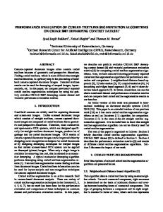
One common insight from the literature is confirmed in this proposition: it is necessary for full JPE to be optimal that all covariances are negative, and it is necessary for for full RPE to be optimal that all covariances are positive. However, this is far from being sufficient. Even when all of the covariances are positive, full RPE may not be optimal (see Figure 1). Note finally that IPE can only occur at the origin in terms of covariances. That is, even if there is no performance correlation in equilibrium, it may still be strictly optimal to use a dependent compensation scheme because there is out-of-equilibrium correlation, which matters for the incentive constraint. The full picture that emerges from this proposition is summarized in Figure 1. It is particularly interesting that mixed schemes are often optimal. These schemes that mix elements of RPE and JPE have clear economic interpretations and are probably the most widespread in practice. They correspond to the combination of profit sharing with selective promotion (in the fourth case) or selective firing (in the fifth case). In most firms, employees are incentivized both through stock participation (a joint component) and promotions (a relative component). On the theoretical side, this suggests that analyses in which the level of relative evaluation is constant over all result pairs, such as the LEN model, are unsatisfactory in that, by design, they preclude the optimality of mixed schemes. This is so because wages are linear in the other agent’s performance, which forces the incentive scheme to always exhibit JPE or always exhibit RPE.12 Proposition 3 will be extended in Section 5.1 to the case of multiple outcomes. This will focus on the fourth kind of scheme, with JPE at the top when correlation increases with effort. We here illustrate the other type of mixed scheme, with RPE at the top, by a simple example. 12 Moreover,
¨ and Milgrom (1987) obtain conditions under which an optimal incentive while Holmstrom
scheme is linear in aggregate profit, there is no result stating that in a model with multiple observables – possibly from different agents – the optimal incentive scheme should be linear in those performances.
13
γ11
p1 p0
RPE
1− p1 1− p0
Relative penalties 45◦
JPE
γ01
Relative bonuses
Figure 1: Optimal schemes in the covariance space when agents are risk-averse. Example 1 Designing a research contest. Consider the case of two researchers in a given field. Effort will here represent the novelty of the approach. Being original most often entails more effort than just following the mainstream – not least because it entails having read the existing work first. In other words, proving that work is original is much harder than proving that it is not. Most importantly, it is assumed that γ00 > γ10 = γ01 > γ11 ≥ 0, which reflects the fact that more originality induces lower correlation. This captures both that effort by any one of
the researchers reduces the correlation, and that researchers are intrinsically differentiated (they become more dispersed as they become more creative). If effort sufficiently reduces correlation, then the optimal scheme is characterized by: wSF > wSS , hence there is competition at the top, and w FS > w FF , hence results are shared at the bottom. As a result, under the optimal incentive scheme, a researcher whose approach fails should receive a higher payoff in an overall more successful field than in an unproductive one.
14
4
Limited Liability and Applications
In this section, we consider optimal incentives in a framework with risk-neutral agents who are subject to limited liability.13 The incentive constraint is the same as that above, with u(.) = Id, while we normalize the liability limit to 0, hence the constraints: w≥0
(6)
A result which is analogous to Lemma 1 holds in this setting. However, given that only linear programming is involved in determining the optimal incentive scheme we obtain corner solutions: Lemma 2 Under risk-neutrality and limited liability, an optimal incentive scheme entails positive wages only for the result(s) with the highest incentive efficiency. This result parallels Lemma 1 for the case of limited liability. The underlying logic is essentially the same, up to the fact that the agent being risk-neutral, there is no need for compensation smoothing. Hence all the incentive weight is put on the result that is most informative regarding effort.
4.1
Information structure
For the results in this section, we introduce technological uncertainty as the source of the covariance. This is one generic way of handling the information structure. The interpretation is that the probabilities of success conditional on effort are not known with certainty. All players hold the same beliefs regarding those probabilities. The success probability of agent i conditional on his effort ei is a random variable, p˜ ei . Since we want to allow for a stochastic link between performances, we have to distinguish between the two agents’ draws of success probability, hence q˜e− i denotes the draw of the other agent. In the following we use the following assumptions and notation: E[ p˜ e ] = E[q˜e ] ≡ pe , 13 We
var ( p˜ e ) = var (q˜e ) ≡ σe2
∀e ∈ {0, 1}
can consider an additional ex-ante participation constraint. However, given the limited liability
requirement, it would be automatically satisfied in the (interesting) cases where moral hazard is costly. Henceforth we shall thus ignore such participation constraints for expositional clarity.
15
so that agents’ projects are ex-ante identical.14 In turn, they may well be different ex-post, ˜ and q’s. ˜ due to different draws of the p’s The following correlation parameters will be used in the analysis: ρ ei e −i ≡
cov( p˜ ei , q˜e−i ) σei σe−i
This is the most general form of imperfect knowledge that we can introduce in the present setting.15 Note that we do not make any assumptions regarding the supports of the p˜ ei ’s, only that they should all be included in [0, 1]. Also note that the correlation coefficients pertain to the beliefs over the distribution of results. Fortunately these coefficients are also proportional to the correlation between outcomes. The covariances used in the previous paragraph of course directly result as: γei e−i = ρei e−i σei σe−i
(7)
This illustrates how the formulation with second-order uncertainty is one possible decomposition of the covariance. Finally, this way of modeling uncertainty in a contractual framework also has the advantage that the noise parameter it introduces is independent of any mechanical effect of effort on variance. Indeed, the variance of performance with a bounded support is intrinsically linked to effort. Consider the particular case of a binomial draw: The (normalized) variance of performance is pe (1 − pe ). We can hence not analyze the pure effect
of variance without considering the mean at the same time. As will become clear, the information structure proposed here allows us on the contrary to consider independently the level of effort and the uncertainty associated with production. 14 Note
however that the case of non-identical agents, e.g. with E[ p˜ e ] 6= E[q˜e can be treated similarly. The
asymmetric case was fully analyzed in a previous version of the paper, but it does not add any particular
insights. 15 This representation of the information structure is of course not unique, since many state space representations could be used (see in particular Conlon, 2009, for a discussion). The game is here viewed as a one-shot multi-arm bandit problem in which ex-post information is used to infer which arms the agents picked. This precisely allows us to center the analysis on generic distributional properties. An alternative structure is taken in Magill and Quinzii (2006), which features idiosyncratic and common shocks. One nice property of their representation is that the distribution of the common shock does not enter their characterization. However the dependence structure cannot easily be analyzed in their setting. The information structure in our model here is also very convenient in that it introduces no restrictions like Assumption 2 in Mookherjee (1984, p. 436) with respect to the dependence structure.
16
4.2
Preliminary results and further assumption
However intuitive Lemma 2 may appear, it does not indicate which wage will be positive. It actually makes possible a number of rather counterintuitive results regarding optimal schemes. The next example illustrates this point. Example 2 Extreme innovation. Consider symmetric agents using identical technologies. Assume that an old well-known technology yields at no cost success with a fixed probability of p0 (= q0 ). On the contrary, the new technology might be either a perfect fit, with a probability of p1 such that p1 > p0 , or be completely useless, with a probability of 1 − p1 . A perfect fit yields success with a probability of 1, while a useless technology produces a failure for sure. Implementing the new technology requires a learning cost of c. Here p˜ 1 (= q˜1 ) has a binomial distribution
with parameter p1 –and consequently a variance of σ12 = p1 (1 − p1 ) > 0. Therefore, we p21 + p1 (1− p1 ) (1− p )2 + σ 2 p21 +σ12 = p10 , h(SF ) = h( FS) = 0 and h( FF ) = (1− p 1)(1− p1 ) = p1 p0 = p1 p0 0 1 p0 > 12 , the highest likelihood ratio is that of a double failure: agents should
have h(SS) = 1 1− p0 .
Thus if
be compensated only in that state. There are thus situations in which agents are rewarded only upon obtaining two failures, such as that described above. While such situations could be worthy of analysis per se,16 we will here rule them out to focus on the standard settings in the literature. This is the role of the next assumption regarding the technology. Assumption 1 (Effective Effort)
Prob( p˜ 1 ≥ p˜ 0 ) = 1
This quite transparent assumption requires that the probability of success be increasing in effort for any technology type. In Example 2 this is not the case, since in some states of nature the technology is such that p˜ 1 = 0 < p0 , i.e. the new technology is not of use. The assumption is stronger than needed for our results, but has the advantage of being simple and meaningful. One nice consequence of Assumption 1 is given below. Lemma 3 Under Assumption 1, an optimal scheme entails w FF = w FS = 0. The assumption implies that failure by agent i is never rewarded whatever the result of agent −i. It suffices to check that under Assumption 1 success is always a better indication of effort than failure. 16 See
for example Manso (2010) for a related one-agent, two-period model in which early failures may
represent good news regarding effort.
17
4.3
Main results with limited liability
We are now in a position to fully characterize the optimal incentive scheme in terms of the informational parameters. Proposition 4 With risk-neutral agents subject to limited liability, under Assumption 1, the optimal wage profile is: 1. Joint performance evaluation when ρ11 σp11 > ρ01 σp00 , with wSS =
c , p1 ( p1 − p0 ) + σ1 (ρ11 σ1 − ρ01 σ0 )
wSF = w FS = w FF = 0
2. Relative performance evaluation when ρ11 σp11 < ρ01 σp00 , with wSF =
c , (1 − p1 )( p1 − p0 ) − σ1 (ρ11 σ1 − ρ01 σ0 )
wSS = w FS = w FF = 0
3. Any scheme (possibly Independent Performance Evaluation) when ρ11 σp11 = ρ01 σp00 , with
( p1 +
σ c σ1 )wSS + (1 − p1 − 1 )wSF = , p0 p0 p1 − p0
w FS = w FF = 0
The criterion for relative vs joint performance evaluation, although it looks very simple, does have rich economic content. On the technical side, it is generic in that it does not put any restriction on the shape of the underlying distributions apart from Assumption 1.17 It depends only on the first two moments, so that it is purely informational. One way to relate this result to Proposition 1 is to identify the type of complementarity properties created by the dependence structure. Looking at the effect that ei has on R−i ,
we have:
p21 + ρ11 σ12 Prob(SS|1, 1) = Prob(SF |1, 1) p1 (1 − p1 ) − ρ11 σ12
which is increasing in ρ11 . On the other hand:
Prob(SS|0, 1) p0 p1 + ρ01 σ0 σ1 = Prob(SF |0, 1) p0 (1 − p1 ) − ρ01 σ0 σ1 which is increasing in ρ01 . Hence increasing ρ11 relative to ρ01 makes the log-supermodularity condition of Proposition 1 more likely to hold. In this sense, Proposition 4 emphasizes that correlation creates a form of informational complementarity. 17 In the multi-agent models mentioned in the introduction, almost all distributions are either multivariate
normal representing additive noise or two-point distributions.
18
Proposition 4 also makes a key connection between two dimensions: first, the correlation conditional on effort and, second, the effect of effort on the variability of the result. In the case of positive correlation, the criterion for JPE can be rewritten as follows: p σ ρ11 > 1 0 ρ01 σ1 p0 The first dimension is a pure multi-agent effect, while the second is a pure single agent effect. The coefficient of variation
σe pe
is a measure18 of how noisy the success signal is
as a function of effort e. If the right-hand side term is less than 1, effort increases this noise, while it reduces noise if it is greater than 1.19 With respect to the correlation, if the ratio
ρ11 ρ01
is greater than 1, the agents’ results are more correlated when they choose the
same actions than when they choose different actions. This ratio is new in multi-agent analysis since previous work has only considered uniform correlation.20 What counts for the choice between RPE and JPE is the relative quality of information between the two possible actions for one agent, and how the correlation between results varies across actions. We end this discussion with one important implication of Proposition 4. Proposition 5 All else equal, an increase in the equilibrium correlation of outcomes favors JPE. Proof. The equilibrium covariance of the two results is cov( p˜ 1 S + (1 − p˜ 1 ) F, q˜1 S + (1 − q˜1 ) F ) = (S − F )2 ρ11 σ12 , while the variances of the results are var ( p˜ 1 S + (1 − p˜ 1 ) F ) =
(S − F )2 σ12 = var (q˜1 S + (1 − q˜1 ) F ). The equilibrium correlation is thus exactly ρ11 , and greater ρ11 makes JPE more attractive, according to Proposition 4. This observation runs counter to the standard results. This is the most striking consequence of the informational complementarity effect. Previous models consider only settings where good performances indicate a favorable environment, hence conclude that this favorable noise should be filtered by RPE. Here an effect that has previously been ignored is at work: a good result for the other agent might also be a good signal of effort under high equilibrium correlation. 18 Various risk measures have been defined in financial analysis.
The inverse of the coefficient of variation
is referred to as the ’Sharpe ratio’ in portfolio analysis. Portfolios with a smaller Sharpe ratios are considered to be riskier, that is noisier in the informational interpretation of the model. 19 Whether exerting more effort increases noise is for instance one of the conditions discussed in the career concern model by Dewatripont et al. (1999): see Example 5 below. 20 Ramakrishnan and Takor (1991) insist on the role of conditional correlation, but as they mention (p. 260), agents take the value of the correlation to be exogenous in their model. It seems reasonable to assume that sophisticated agents will take into account the fact that this correlation will vary with their own choice of action.
19
Remark 1 The principal always benefits from uncertainty over technology as long as it is not independent across agents. The principal’s expected gains do not depend on uncertainty. While, with perfect knowledge of the technology, the principal would use independent schemes, when knowledge is imperfect he can still use a pair of independent contracts (IPE) but that it is no longer optimal. Therefore the costs are lower with RPE or JPE and the principal benefits from the uncertainty. The literature has already noted a number of times that correlation helps to reduce the cost of moral hazard and facilitates information revelation. Here, the same conclusion can be drawn with respect to uncertainty in general, provided all the players are risk-neutral.
4.4
Examples
To illustrate the main result, we briefly apply it to the typical types of uncertainty that have been considered in the literature. The optimal scheme is RPE in Examples 3 and 4, while it is IPE or JPE in Examples 5 and 6. Example 3 The additive model. The most classic way of introducing technological uncertainty in our discrete model is as follows: p˜ ei = pei + ε q˜e−i = pe−i + η where ε and η are random variables with zero means, variances of σ2 and a correlation coefficient of ρ. What matters here is that the noise is additively separable from the influence of the action. Note that the variance of the probability of success depends only on ε, which implies that σ0 = σ1 . All pairs ( p˜ ei , q˜e−i ) have the same correlation of ρ. Also, σ0 p1 p0 σ1
= pp10 > 1. Therefore, from Proposition 2, RPE is always optimal with additive uncertainty. That formulation of additive uncertainty parallels that in Lazear and Rosen (1981) and Nalebuff and Stiglitz (1983). We have shown that this setting favors competition between agents, even abstracting from risk-sharing concerns. Example 4 Effort is sometimes irrelevant.
20
Che and Yoo (2001) use an original information structure. They assume that with some probability ν the technology is such that a project is a success regardless of effort,21 and that with probability (1 − ν) the outcome will depend on effort. We denote the probability of success in the latter case by re . Overall, this corresponds to the situation: ( {1, 1} with probability ν { p˜ 0 , p˜ 1 } = {q˜0 , q˜1 } = {k0 , k1 } with probability (1 − ν) The relationships with our notation are simply: ke =
pe − ν , 1−ν
Therefore, since we here have setting.22
σe2 =
ν (1 − p e )2 1−ν
p1 (1− p0 )2 p0 (1− p1 )2
and
ρ ei e −i = 1
> 1, RPE is the optimal incentive scheme in this
Example 5 The multiplicative model. Consider the following setup where the probability of an agent’s success is given by: p˜ ei = εpei q˜e−i = η pe−i where ε and η are random variables with means of 1, variances of σ2 and a correlation of ¨ (1982) and also ρ. This functional form of uncertainty is used as an example in Holmstrom appears in the career concerns model (e.g. Dewatripont et al., 1999). Note that all pairs ( p˜ ei , q˜e−i ) have the same correlation of ρ, so that ρρ11 = 1. In addition we have σ0 = p0 σε 01
and σ1 = p1 σε . Hence, applying the third bullet of Proposition 4, IPE is an optimal scheme here (but not the unique one, as seen in the proposition). Note that this is true for any level of equilibrium correlation ρ. Example 6 Stock-options in startups. 21 It is unimportant
that the probabilities be exactly 1, what matters is that they are the same in some state
of the world, making effort irrelevant in that state. 22 To be clear, the contribution of Che and Yoo (2001) is to show that, while RPE is optimal in this static setting, JPE becomes optimal in the infinitely-repeated version of the problem. Proposition 4 gives a full answer to their footnote 16 (pp. 530-531), regarding how the form of the common shocks affects the RPE vs JPE choice in the static setting.
21
As a last application, consider the problem of inducing innovation in a new technological venture. A status quo solution consists in using an old, known technology, which generates a success with fixed probabilities p0 and q0 (so that σ0 = 0). In turn, the agents can innovate, at a cost of c, in order to use a new, imperfectly-known technology, with a ranρ dom probability of success of p˜ 1 = q˜1 . In that case, ρ11 tends to infinity, and Proposition 4 01
indicates that the optimal way of providing incentives to innovate is to use a JPE scheme. There are admittedly many other reasons behind the use of stock options in startups, but this example shows that it may even be profitable for a principal (say, a venture capitalist) to incentivize collectively the startup members for purely informational reasons.
5
Extensions
5.1
Mixed schemes with multiple outcomes
This section considers the case of multiple outcomes. There are now n performance levels: Ri ∈ { X 1 ...X n }, with everything else as in Section 3. The joint distribution of the pair of outcomes is given by Prob( Ri , R−i |ei , e−i ), hence all the notation used above carry
through. In particular, the incentive efficiency of w R is still defined as in Definition 2. We can appeal to the results obtained above, since Lemma 1 applies equally well to this richer outcome space. We hence want to analyze how h( R) varies with the pair of outcomes R, and in particular with R−i . Accordingly, we provide a local definition of JPE and RPE that
fits the many-outcome setting:23
Definition 3 (local JPE and RPE) An incentive scheme exhibits Relative Performance Evaluation for a given result Ri of agent i when: w Ri R−i is decreasing in R−i An incentive scheme exhibits Joint Performance Evaluation for a given result Ri of agent i when: w Ri R−i is increasing in R−i An appealing form of mixed schemes can be characterized simply: those that have only elements of RPE and JPE for a given level of performance.24 The following is an 23 Definition 24 I
1 is stronger in that it requires JPE or RPE to hold for any result of agent i. am grateful to a referee for providing the motivation for the analysis of these contracts.
22
adaptation of an assumption proposed by Szalay (2009) in the context of information acquisition in an adverse-selection model.25 Assumption 2 (’Reversing’ monotone likelihood ratio) There exist X ∗ ∈ { X 1 ...X n } such that h( Ri , R−i ) is increasing in R−i for all Ri such that Ri ≥ X ∗ and decreasing for Ri < X ∗ .
Note that we can also treat the case of a monotone likelihood ratio that is first increasing then decreasing. The following proposition characterizes the optimal incentive schemes using this assumption: Proposition 6 The optimal incentive scheme is RPE for Ri < X ∗ and JPE for Ri ≥ X ∗ if and only if the distribution of outcomes satisfies Assumption 2 at X ∗ .
The scheme is thus a ”Relative Penalties” contract of Proposition 3. The assumption of a reverting monotone likelihood ratio is however fairly strong (an example is given below), and illustrates that this type of scheme is rather particular. Moreover it is not transparent in terms of correlation. In order to confirm the main insights on the effect of positive dependence with multiple outcomes we look at another framework. In particular we will not impose any assumptions on the likelihood ratio but only on the dependence structure. First, we assume the technological independence of production (see (5)), in order to concentrate on the informational dimension. We assume the following regarding the statistical dependence of outcomes: Assumption 3 (informational independence with different efforts) Prob( Ri , R−i |0, 1) = Prob( Ri |0) Prob( R−i |1)
∀( Ri , R−i )
Assumption 4 (affiliation with high efforts) Prob( Ri , R−i |1, 1) Prob( Ri0 , R0−i |1, 1) ≥ Prob( Ri0 , R−i |1, 1) Prob( Ri , R0−i |1, 1)
∀( Ri , R−i , Ri0 , R0−i ) s.t. Ri ≤ Ri0 , R−i ≤ R0−i
Under those assumptions, the outcomes of the agents are fully independent when the agents choose different efforts, but are positively related when they both work. This is therefore a generalization of the examples mentioned in the introduction and Example 6. The next proposition focuses on the generalization of the ”Relative Penalties” of 25 See
Szalay (2009) equation (17), p.197, and the associated discussion.
23
Proposition 3, i.e. the fourth case, featuring JPE at the top and RPE at the bottom. This comes about when the equilibrium correlation is sufficiently high compared to out-ofequilibrium correlation, which is what the previous assumptions capture. The flavor of the result confirms the intuition obtained in the two-outcome case. Proposition 7 Under Assumptions 3 and 4, there exist X ∗ and X ∗∗ such that the optimal contract exhibits JPE when Ri ≥ X ∗ and RPE when Ri ≤ X ∗∗ . The intuition is that affiliation (the natural form of dependence in a context where the likelihood ratio matters) entails that the distribution has on average higher weights along the diagonal, compared to the case of independence. For high outcomes of i, this means that the weight is shifted towards high outcomes of −i, and conversely for low re-
sults. The proposition shows that for sufficiently extreme outcomes, this shift of weights necessarily creates an always increasing (or always decreasing) likelihood ratio. The last example kills two birds with one stone: the first part illustrates Proposition 7, while the second is a slight modification in which mixed schemes as in Proposition 6 can be obtained under the same set of assumptions. Example 7 (three outcomes) Let n = 3, and let Prob( Ri |ei ) be given by the following table: ei \
Ri
X1
X2
X3
0
1 3 2 9
1 3 1 3
1 3 4 9
1
Prob( Ri |ei ) which has an increasing likelihood ratio (note that this is not required for Proposition 6 to hold). The probabilities Prob( Ri , R−i |0, 1) are obtained using independence (assumption
3) in the first table. Following Assumption 4, we assume in the second table that the
outcomes are affiliated when ei = e−i = 1. The relevant likelihood ratios can then be
computed in the third table. The corresponding tables are shown below:
24
Ri \
R −i
X1
X2
X3
X1
6 81 6 81 6 81
9 81 9 81 9 81
12 81 12 81 12 81
X2 X3
Ri \
R −i
X1
X2
X3
X1
9 81 5 81 4 81
5 81 10 81 12 81
4 81 12 81 20 81
X2 X3
Prob( Ri , R−i |0, 1)
Ri \
R −i
X1
X2
X3
X1
3 2 5 6 2 3
5 9 10 9 4 3
1 3
X2 X3
Prob( Ri , R−i |1, 1)
1 5 3
h ( Ri , R −i )
It is easily checked that outcomes are affiliated in the second table. In the third table, increasing cells from left to right imply JPE, and decreasing cells imply RPE. We can see that the optimal wage is RPE at Ri = X 1 , and JPE at Ri = X 3 , while it is neither JPE nor RPE at Ri = X 2 . Now, suppose we change the distribution when (e1 , e2 ) = (1, 1) as follows, with only the bottom-right square being modified (in bold): Ri \
R −i
X1
X2
X3
X1
9 81 5 81 4 81
5 81 9 81 13 81
4 81 13 81 19 81
X2 X3
Ri \
R −i
X1
X2
X3
X1
3 2 5 6 2 3
5 9
1 3 13 12 19 12
X2 X3
Prob( Ri , Ri |1, 1)
1 13 9
h ( Ri , Ri )
These likelihood ratios satisfy Assumption 5, and Proposition 6 applies. The outcomes are still affiliated, and now the scheme is of the ”Relative Penalties” kind, with RPE for Ri = X 1 and JPE for all higher results.
5.2
Continuous effort and First-Order Approach
This section extends the model to continuous effort, and provides a set of natural conditions for the first-order approach to hold. Following the spirit of the first-order approach, the goal will be to study the least costly way of implementing any given effort pair (then the omitted second step consist in selecting that which is the most efficient among implementable effort pairs). The model features continuous effort (ei , e−i ) ∈ [0, 1]2 and a binary outcome. The
agents are risk-averse, and subject to an ex-ante participation constraint. We use the same notation as above whenever possible. In particular, we use the unambiguous notations 25
p(ei ), c(ei ) and γ(ei , e−i ) to denote the independent probability of success, the cost of
effort and normalized covariance, respectively. Agents are symmetric, so that the indi-
vidual success probabilities are determined by the same function p. Hence, the probabilities26 of the various outcomes are given by the following matrix: Ri \
R −i
F
S
(1 − p(ei ))(1 − p(e−i )) + γ(ei , e−i ) (1 − p(ei )) p(e−i ) − γ(ei , e−i ) S p(ei )(1 − p(e−i )) − γ(ei , e−i ) p ( ei ) p ( e −i ) + γ ( ei , e −i )
F
In the following, subscripts pertain to derivatives. We will impose the following standard assumptions: the function p is increasing and concave with lime→0 p0 (0) = +∞; and 0 < p(.) < 1, so that the optimal effort in the absence of moral hazard is interior. This implies decreasing returns to effort in the case of fully independent production, but does not imply a monotone likelihood ratio in own result for all pair of efforts. Finally, we assume that the function c is increasing and convex. In order to use the first-order approach, we require additional assumptions regarding the covariance which are introduced as we proceed. The expression below shows the likelihood ratios that are relevant in this continuous-effort setting: J ( R | ei , e −i ) ≡
d log ( Prob( R|ei , e−i )) dei
We now turn to the first-order approach and its justification, following the lines of Rogerson (1985), extended to the present multi-signal case by Sinclair-Desgagn´e (1994) and more recently by Conlon (2009). Consider the solution to the relaxed problem of the principal, i.e. where we replace the incentive constraint by the less demanding requirement that the agent’s utility be at a stationary point. We associate the Lagrange multipliers λ and µ, to, respectively, the relaxed incentive constraint and the participation constraint. Assuming that the expected utility of the agent is concave, the wage should satisfy the usual equation featuring the likelihood ratio, namely: 1 u0 (w
R)
= µ + λJ ( R|ei , e−i )
(8)
Hence wages are ranked in the same way as the J’s. However, so far the properties of p are not sufficient to imply any sort of monotone likelihood ratio, nor have we shown that the agent’s utility is indeed concave. To that end we require the following: 26 This
entails of course some feasibility restrictions on γ, namely: 0 ≤ p(ei ) p(e−i ) + γ(ei , e−i ) ≤ 1,
0 ≤ p(ei )(1 − p(e−i )) − γ(ei , e−i ) ≤ 1, and 0 ≤ (1 − p(ei ))(1 − p(e−i )) + γ(ei , e−i ) ≤ 1 for all (ei , e−i ).
26
Assumption 5 (Uniformly effective efforts) For all (ei , e−i ): p(e−i ) p0 (ei ) + γei (ei , e−i ) ≥ 0 and (1 − p(e−i )) p0 (ei ) − γei (ei , e−i ) ≥ 0 This simply says that for any effort of the other agent, own effort is always marginally productive. This assumption is an adaptation of Assumption 1 and serves the same purpose as in the discrete model: it guarantees that failures are never better rewarded than are successes. Indeed it is routine to check that this assumption implies J (SS|ei , e−i ) ≥
J ( FS|ei , e−i ) and J (SF |ei , e−i ) ≥ J ( FF |ei , e−i ). Note in passing that in the setting with risk-
neutral agents subject to limited liability this assumption would lead to a result analogous to Lemma 3. Hence the analysis of Section 4 also generalizes to continuous effort.
We now show that the first-order approach is valid under a last sufficient assumption. The expected utility of the agent under an incentive scheme w is still formally given by (1), and its second derivative with respect to e is: d2 (Ui (w|ei , e−i )) = p00 (ei ) [ p(e−i )(u(wSS ) − u(wSF )) + (1 − p(e−i ))(u(wSF ) − u(w FF ))] dei2
+ γei ei (ei , e−i ) [u(wSS ) − u(wSF ) + u(wSF ) − u(w FF )] − c00 (ei ) We now state: Assumption 6 γ(., .) is concave in its first argument. To conclude, under Assumption 5, the solutions to (8) are such that wSS ≥ w FS and wSF ≥ w FF . Using in addition Assumption 6 implies
is complete:
d2 dei2
(Ui (w|ei , e−i )) < 0, hence the argument
Proposition 8 Under Assumptions 5 and 6, the first-order approach is justified and the optimal wages satisfy equation (8). We can now investigate the properties of the optimal incentive scheme as given by the ranking of the likelihood ratios. Determining whether the optimal scheme is RPE or JPE amounts to comparing J (SS|ei , e−i ) to J (SF |ei , e−i ) and J ( FS|ei , e−i ) to J ( FF |ei , e−i ). Straightforward algebra yields:
J (SS|ei , e−i ) > J (SF |ei , e−i ) ⇔ γei (ei , e−i ) p(ei ) > γ(ei , e−i ) p0 (ei ) and: J ( FS|ei , e−i ) > J ( FF |ei , e−i ) ⇔ γei (ei , e−i )(1 − p(ei )) < γ(ei , e−i ) p0 (ei ) 27
It is notable that these criteria are direct (local) translations in continuous terms of those found in Proposition 3. Hence the same interpretation and comments apply to this case of continuous effort. What matters here is how much correlation is relatively affected by a change in effort, as compared to how much the probability of success is relatively affected. For instance, assuming that correlation is (locally) increasing in effort, the first inequality can be rewritten as : γe i ( e i , e − i ) p 0 ( ei ) > γ ( ei , e −i ) p ( ei ) which says that joint performance evaluation at the top is optimal when correlation increases sufficiently with effort.
6
Conclusion
The message of this paper is twofold. First, the presumed optimality of relative performance evaluation when performances are positively correlated required thorough reassessment. The model here has demonstrated that standard results in multi-agent moralhazard problems are not robust, and identifies the particularity of previous analyses. For instance, under risk-neutrality, an increase in the equilibrium correlation of performances favors joint performance evaluation. Second, since correlated risks call for noise filtering through relative performance evaluation with risk-averse agents, two opposing effects have to be traded off when designing multi-agent incentive packages. Optimal mixed schemes balancing those two effects typically exhibit features of real-life contracts that previously lacked theoretical foundations. The optimal mix of competitive and collaborative incentives in firms is a promising research topic. The application of these results to the much-debated issue of the remuneration of top executives and fund managers would also seem to be of considerable interest.
28
A
Omitted Proofs
A.1
Proof of Lemma 1
We associate the positive multipliers λ ≥ 0 and µ ≥ 0 to, respectively, the incentive and participation constraints, and form the Lagrangian of the cost minimization problem: L(w, λ, µ) = Σ R Prob( R|11)w R + λc + µ(U + c)
−Σ R [λ ( Prob( R|11) − Prob( R|01)) + µProb( R|11)] u(w R )
From the usual considerations, both multipliers have to be positive. The first-order conditions w.r.t. the w R boil down to: Prob( R|11) − Prob( R|01) 1 = µ + λ = µ + λI ( R) u0 (w R ) Prob( R|11) Note that
1 u0
is an increasing function, thus the ws are ranked in the same way as
1 . u0 (w)
Hence wages are ranked according to their incentive efficiency.
A.2
Proof of Proposition 1
Consider the case of log-supermodular production. By definition, we have: Prob(SS|0, 1) Prob(SS|1, 1) Prob(SF |1, 1)) Prob(SS|1, 1) ≥ ⇔ ≥ Prob(SF |1, 1) Prob(SF |0, 1) Prob(SS|0, 1) Prob(SF |0, 1)
⇔ h(SS) ≥ h(SF )
and Prob( FS|1, 1) Prob( FS|0, 1) Prob( FS|1, 1) Prob( FF |1, 1)) ≥ ⇔ ≥ Prob( FF |1, 1) Prob( FF |0, 1) Prob( FS|0, 1) Prob( FF |0, 1)
⇔ h( FS) ≥ h( FF )
Note that we have used equivalences, hence the conclusion follows from Lemma 1. The case of log-submodularity is dealt with similarly.
A.3
Proof of Proposition 2
We need to compare h(SS) to h(SF ) and h( FS) to h( FF ): h(SS) − h(SF ) =
p211 p (1 − p11 ) p p − p10 − 11 = 11 11 p01 p10 p01 (1 − p10 ) p01 p10 (1 − p10 ) 29
h( FS) − h( FF ) =
(1 − p11 )2 1 − p11 p11 − p10 p11 (1 − p11 ) − = (1 − p01 ) p10 (1 − p01 )(1 − p10 ) 1 − p01 p10 (1 − p10 )
both of which amount to comparing p11 and p10 , hence the conclusion.
A.4
Proof of Proposition 3
The ranking between wSS and wSF corresponds to the criterion of the heuristic approach, which is derived as follows: p21 + γ11 p (1 − p1 ) − γ11 h(SS) > h(SF ) ⇔ > 1 p0 p1 + γ01 p0 (1 − p1 ) − γ01
⇔ γ11 p0 > γ01 p1
To finish the proof, we want to establish the ranking of w FF and w FS , which requires a similar calculation: p1 (1 − p1 ) − γ11 (1 − p1 )2 + γ11 h( FS) > h( FF ) ⇔ > p0 (1 − p1 ) − γ01 (1 − p0 )(1 − p1 ) + γ01
⇔ γ11 (1 − p0 ) < γ01 (1 − p1 )
Combining those two inequalities yields the desired conclusion.
A.5
Proof of Lemma 2
In the principal’s program, let λ > 0 be the Lagrange multiplier associated with the incentive constraint, and µR ≥ 0 that associated with the limited liability constraint wR ≥
0. The first-order condition for each wR is:
− Prob(R|1, 1) + λ( Prob(R|1, 1) − Prob(R|0, 1)) + µR = 0 If a wage wR is positive then µR = 0 and the last equation is written as: I (R) =
1 λ
For a wage equal to zero, say wR’ , we have I (R’) = conclusion.
30
1 λ (1
−
µR’ ) Prob(R’|1,1)
<
1 λ,
hence the
A.6
Proof of Lemma 3
By complementary probabilities and independent production, we have the identities: Prob(SS|1, 1) − Prob(SS|0, 1) = − ( Prob( FS|1, 1) − Prob( FS|0, 1))
Prob(SF |1, 1) − Prob(SF |0, 1) = − ( Prob( FF |1, 1) − Prob( FF |0, 1)) so that the incentive constraint can be written as:
( Prob(SS|1, 1) − Prob(SS|0, 1))(wSS − w FS )
+ ( Prob(SF |1, 1) − Prob(SF |0, 1))(wSF − w FF ) ≥ c
Now, we have: Prob(SS|1, 1) − Prob(SS|0, 1) = E[ p˜ 1 q˜1 ] − E[ p˜ 0 q˜1 ] = E[q˜1 ( p˜ 1 − p˜ 0 )] From Assumption 1, ( p˜ 1 − p˜ 0 ) is a positive random variable, as is q˜1 . Thus the coefficient on w FS in the incentive constraint is negative, which implies that this wage should be 0. Similarly, we have: Prob(SF |1, 1) − Prob(SF |0, 1) = E[ p˜ 1 (1 − q˜1 )] − E[ p˜ 0 (1 − q˜1 )]
= E[(1 − q˜1 )( p˜ 1 − p˜ 0 )]
which is also positive from the assumption, hence w FF also has to be 0.
A.7
Proof of Proposition 4
From lemmata 2 and 3, we know that except in the special case I (SS) = I (SF ) only one wage is positive. The criterion for wSS > 0 is I (SS) > I (SF ). We require the following simple calculations to undertake the comparison: Prob(SS|11) = E[ p˜ 1 q˜1 ] = p21 + ρ11 σ12
Prob(SS|01) = E[ p˜ 0 q˜1 ] = p0 p1 + ρ01 σ0 σ1
Prob(SF |11) = E[ p˜ 1 (1 − q˜1 )] = p1 (1 − p1 ) − ρ11 σ12
Prob(SF |01) = E[ p˜ 0 (1 − q˜1 )] = p0 (1 − p1 ) − ρ01 σ0 σ1
Using these values yields: h(SS) > h(SF ) ⇔
p1 (1 − p1 ) − ρ11 σ12 p21 + ρ11 σ12 > p0 p1 + ρ01 σ0 σ1 p0 (1 − p1 ) − ρ01 σ0 σ1 31
which simply boils down to ρ11 > ρ01
p1 σ0 σ1 p0
Conversely, we easily obtain that wSF is positive under the reverse inequality. The optimal wages are then straightforwardly obtained by saturating the incentive constraint. In the case of equality, both wages have the same incentive weight, and only their sum matters. The optimal sum is obtained by saturating the incentive constraint.
A.8
Proof of Proposition 7
We prove only the first part of the proposition, as the other obtains analogously. Since Lemma 1 applies just as well with multiple outcomes, the condition for local JPE at Ri can be written as follows: for any R−i and R0−i such that R0−i ≥ R−i , we have: h ( Ri , R −i ) ≤
h( Ri , R0−i )
Prob( Ri , R0−i |11) Prob( Ri , R0−i |01) Prob( R0−i |1) ⇔ ≥ = Prob( Ri , R−i |11) Prob( Ri , R−i |01) Prob( R−i |1)
where the last equality comes from full independence in the case of different efforts (Assumption 3). Now fix a pair ( R−i , R0−i ) with R0−i > R−i . Note that: n
∑ Prob(X j , R−i |11) Prob( R0−i |1) = Prob( R−i |1) Prob( R0−i |1)
j =1
n
=
∑ Prob(X j , R0−i |11) Prob( R−i |1).
j =1
Hence it can not be the case that for all Ri : Prob( Ri , R0−i |11) Prob( R−i |1) < Prob( Ri , R−i |11) Prob( R0−i |1), otherwise the previous equality would be violated. On the contrary there must exist some X ∗ ( R−i , R0−i ) such that for that given pair ( R−i , R0−i ), Prob( X ∗ ( R−i , R0−i ), R0−i |11) Prob( R−i |1) ≥ Prob( X ∗ ( R−i , R0−i ), R−i |11) Prob( R0−i |1). Now, note that affiliation (Assumption 4) implies that: Prob( Ri , R0−i |11) is nondecreasing in Ri when R0−i ≥ R−i Prob( Ri , R−i |11) so that for all Ri ≥ X ∗ ( R−i , R0−i ), the optimal scheme has to satisfy h( Ri , R−i ) ≤ h( Ri , R0−i ). To finish the proof, take the max of the X ∗ ( R−i , R0−i )’s over all pairs ( R−i , R0−i ). This is 32
a finite set, so that there exists some X ∗ such that JPE obtains at all results Ri ≥ X ∗ . As
long as the affiliation Assumption 4 holds strictly for at least two pairs or outcomes, i.e.
outcomes are not independent, the optimal scheme has a strict JPE component at the top. The proof for the RPE component proceeds similarly.
References Aggarwal, R., Samwick, A., 1999. Executive Compensation, Strategic Competition, and Relative Performance Evaluation: Theory and Evidence, Journal of Finance 54, 19992043. Alchian, A., Demsetz, H., 1972. Production, Information Costs, and Economic Organization, American Economic Review 62, 777-795. d’Aspremont, C., G´erard-Varet, L.-A., 1998. Linear Inequality Methods to Enforce Partnerships under Uncertainty: An Overview, Games and Economic Behavior 25, 311-336. Brusco, S., 1997. Implementing Action Profiles when Agents Collude, Journal of Economic Theory 73, 395-424. Celentani, M., Loveira, R., 2006. A Simple Explanation of the Relative Performance Evaluation Puzzle, Review of Economic Dynamic 9, 525-540. Che, Y.K., Yoo, S.-W., 2001. Optimal Incentives for Teams, American Economic Review 91, 525-541. Conlon, J., 2009. Two New Conditions Supporting the First-Order Approach to Multisignal Principal-Agent Problems, Econometrica 77, 249-278. Demski, J., Sappington, D., 1984. Optimal incentive contracts with multiple agents, Journal of Economic Theory 33, 152-171. Dewatripont, M., Jewitt, I., Tirole, J., 1999. The Economics of Career Concerns, Part 1 and Part 2, Review of Economic Studies 66, 183-217. Green, J., Stokey, N., 1983. A Comparison of Tournaments and Contracts, Journal of Political Economy 91, 349-364.
33
Gromb, D., Martimort, D., 2007. Collusion and the organization of delegated expertise, Journal of Economic Theory 137, 271-299. Himmelberg, C., Hubbard, R., 2000. Incentive Pay and the Market for CEOs: An Analysis of Pay-for-performance Sensitivity, mimeo Columbia Business School. ¨ Holmstrom, B., 1979. Moral Hazard and Observability, Bell Journal of Economics 10, 7491. ¨ B., 1982. Moral Hazard in Teams, Bell Journal of Economics 13, 324-340. Holmstrom, ¨ B., Milgrom, P., 1987. Aggregation and Linearity in the Provision of IntertemHolmstrom, poral Incentives, Econometrica 55, 303-328. ¨ Holmstrom, B., Milgrom, P., 1990. Regulating Trade Among Agents, Journal of Institutional and Theoretical Economics 146, 85-105. Itoh, H., 1991. Incentives to Help in Multi-Agents Situations, Econometrica 59, 611-636. Itoh, H., 1992. Cooperation in Hierarchical Organizations: an Incentive Perspective, Journal of Law, Economics and Organization 8, 321-345. Laffont, J.-J., Martimort, D., 2002. The Theory of Incentives, Princeton University Press, Princeton, NJ. Lazear, E., 1989. Pay Equality and Industrial Politics, Journal of Political Economy 97, 561-580. Lazear, E., Rosen, S., 1981. Rank-Order Tournaments as Optimum Labor Contracts, Journal of Political Economy 89, 841-864. Luporini, A., 2006. Relative performance evaluation in a multi-plant firm, Economic Theory 28, 235-243. Ma, C.-T., 1988. Unique implementation of incentive contracts with many agents, Review of Economic Studies 55, 555-572. Ma, C.-T., Moore, J., Turnbull, S., 1988. Stopping agents from ”cheating”, Journal of Economic Theory 46, 355,372.
34
Magill, R., Quinzii, M., 2006. Common Shocks and Relative Compensation, Annals of Finance 2, 407-420. Manso, G., 2010. Motivating Innovation, Journal of Finance, forthcoming. Maskin, E., Qian, Y., Xu, C., 2000. Incentives, Information and Organizational Form, Review of Economic Studies 67, 358-378. Mookherjee, D., 1984. Optimal Incentives Schemes with Many Agents, Review of Economic Studies 51, 433-446. Nalebuff, G., Stiglitz, J., 1983. Prices and Incentives: Towards a General Theory of Compensation and Competition, Bell Journal of Economics 14, 21-43. Ramakrishnan, R., Takor, A., 1991. Cooperation versus Competition in Agency, Journal of Law, Economics and Organization 7, 248-283. Rogerson, W., 1985. The First-Order Approach to Principal-Agent Problems, Econometrica 53, 1357-1367. Sinclair-Desgagn´e, B., 1994. The First-Order Approach to Multi-Signal Principal-Agent Problems, Econometrica 62, 459-465. Szalay, D., 2009. Contracts with endogenous information, Games and Economic Behavior 65, 586-625.
35