Cross-Institutional Evaluation of BI-RADS Predictive Model for Mammographic Diagnosis of Breast Cancer Joseph Y. Lo 1,2 Mia K. Markey 1,2 Jay A. Baker 1 Carey E. Floyd, Jr. 1,2

OBJECTIVE. Given a predictive model for identifying very likely benign breast lesions on the basis of Breast Imaging Reporting and Data System (BI-RADS) mammographic findings, this study evaluated the model’s ability to generalize to a patient data set from a different institution. MATERIALS AND METHODS. The artificial neural network model underwent three trials: it was optimized over 500 biopsy-proven lesions from Duke University Medical Center or “Duke,” evaluated on 1,000 similar cases from the University of Pennsylvania Health System or “Penn,” and reoptimized for Penn. RESULTS. Trial A’s Duke-only model yielded 98% sensitivity, 36% specificity, area index (Az) of 0.86, and partial Az of 0.51. The cross-institutional trial B yielded 96% sensitivity, 28% specificity, Az of 0.79, and partial Az of 0.28. The decreases were significant for both Az ( p = 0.017) and partial Az ( p < 0.001). In trial C, the model reoptimized for the Penn data yielded 96% sensitivity, 35% specificity, Az of 0.83, and partial Az of 0.32. There were no significant differences compared with trial B for specificity (p = 0.44) or partial Az (p = 0.46), suggesting that the Penn data were inherently more difficult to characterize. CONCLUSION. The BI-RADS lexicon facilitated the cross-institutional test of a breast cancer prediction model. The model generalized reasonably well, but there were significant performance decreases. The cross-institutional performance was encouraging because it was not significantly different from that of a reoptimized model using the second data set at high sensitivities. This study indicates the need for further work to collect more data and to improve the robustness of the model.

T

Received May 15, 2001; accepted after revision August 8, 2001. The opinions and assertions contained herein are the private views of the authors and are not to be construed as official or as reflecting the views of the Department of the Army, the Department of Defense, the National Institutes of Health, or the National Cancer Institute. Supported in part by the following grants: U.S. Army Medical Research and Materiel Command DAMD17-94-J4371, DAMD17-96-1-6226, and DAMD17-99-1-9174; NIH/NCI R29-CA75547 and R21-CA81309; Susan G. Komen Breast Cancer Foundation BCTR00-000730; and Whitaker Foundation RG 97-0322. 1

Department of Radiology, Duke University Medical Center, DUMC–3302, Bryan Research Bldg., Rm. 161G, Durham, NC 27710. Address correspondence to J. Y. Lo.

2

Department of Biomedical Engineering, Duke University, Durham, NC 27710.

AJR 2002;178:457–463 0361–803X/02/1782–457 © American Roentgen Ray Society

AJR:178, February 2002

he low specificity of mammography results in the biopsy of many benign lesions. Only 15–34% of women who undergo biopsy for a mammographically suspicious nonpalpable lesion actually have a malignancy by histologic diagnosis [1, 2]. The excessive biopsy of benign lesions raises the cost of mammographic screening [3] and results in emotional and physical burden to patients. As one approach to improve the accuracy of mammography, many investigators have proposed computer aides to help radiologists detect [4–6] or classify suspicious breast lesions [7– 10]. These techniques may provide immediate and accurate predictions, while being low cost and completely noninvasive. In previous work at this institution, artificial neural network models were developed to identify very likely benign breast lesions, so that biopsy may potentially be avoided in favor of short-term follow-up [11, 12]. Note that these cases may not necessarily be limited to those considered “probably benign” in clinical practice [13].

These models take into consideration the descriptions of lesion morphology according to the American College of Radiology’s Breast Imaging Reporting and Data System (BIRADS) [14], as interpreted by mammographers, and data pertaining to patient history. The models performed at a level comparable to or better than the overall performance of the expert mammographers who originally interpreted the mammograms. The BI-RADS lexicon was designed to standardize mammography reporting [15, 16]. This origin suggested that the model should perform similarly regardless of which radiologist determines the input features. To evaluate the effect of such interobserver variability, each of five radiologists with wide ranges of experience reviewed a subset of 60 cases. This preliminary study found that the interobserver variability for interpretation of the lesions was significantly reduced by the computer models [17]. This finding showed the robustness of such models and suggested their potential applicability when 457

Lo et al. used by radiologists not involved with training the model or even radiologists at other institutions, as long as they all adhered to BI-RADS reasonably consistently. Materials and Methods Research Plan The purpose of our study was to evaluate how well the aforementioned breast cancer predictive model generalized to data from another institution that also used the BI-RADS standard. The artificial neural network model was developed using patient data from our institution, Duke University Medical Center, as interpreted by radiologists at our institution. Hereafter this will be referred to as the “Duke” data set. With no further optimization or adjustments, the model was evaluated using patient data from the University of Pennsylvania Health System as interpreted by the radiologists at that institution, hereafter known as the “Penn” data set. Finally, a new model was customized specifically for the Penn data set to establish an upper bound for performance using that institution’s data. The hypothesis was that the original model optimized at one institution would perform similarly at a different institution. Performances of each of these three experiments were measured using receiver operating characteristic (ROC) analysis. Patients Two independent patient data sets were used for this study. The Duke data set from our institution was used for original development of the models, whereas the Penn data set was used for the cross-institutional trials. The two institutions were both major academic hospitals. All reviewers at both institutions were dedicated breast imaging radiologists. All cases in both data sets consisted of women with mammographically suspicious breast lesions who underwent needle localization and open excisional biopsy to obtain definitive histopathologic diagnosis. Original studies were performed in accordance with standard clinical indications. All

TABLE 1

Comparison of Two Data Sets Used in Cross-Institutional Study

Data Set Name Total number of cases Malignancies (%) Mean age (yr) Age range (yr) Calcification cases Mass cases Mass with calcifications Cases with neither Incomplete cases

458

Duke

Penn

500 174 (35%) 55.5 24– 86 38% 46% 6%

1,000 396 (40%) 55.2 17–92 47% 47% 1%

9% <1%

<1% 5%

data from human subjects were collected retrospectively with approval from appropriate institutional review boards. The Duke data set consisted of 500 localizations from 478 patients between 1991 and 1996. Each case was randomly interpreted by one of seven different mammographers with no overlap. The Penn data set consisted of 1,000 localizations from 997 patients between 1990 and 1997. The Penn cases were similarly interpreted by one of 11 mammographers with no overlap. More information about each data set, including the positive predictive value and mean age, may be found in Table 1 and the Results section. The process for acquiring and encoding the findings was reported previously [11]. In brief, each patient’s films were retrospectively reviewed by one mammographer who was blinded to the biopsy outcome. The mammographer described nine BIRADS lesion morphology findings: mass margin, mass shape, mass density, mass size, calcification morphology, calcification distribution, associated findings, special cases, and lesion location. The calcification number and patient age were also recorded to yield 11 total findings. Although other history data were also recorded, because of a lack of standards, there were differences in the definitions of these variables at the two institutions. Given previous work that suggested that these other history data provided relatively little contribution [12], they were eliminated from consideration in this study. Predictive Modeling and Sampling The methods of developing the computer models have been described in previous studies and will only be summarized here [11, 12]. The models were threelayer (one hidden layer), feed-forward, and error back-propagation artificial neural networks. During training, the network was presented with the input findings for each case and the corresponding known biopsy outcome. The network merged all the findings nonlinearly to generate a single output value between zero and one corresponding to its prediction of the likelihood of malignancy for that case. The network learned iteratively under this supervised training process to improve its performance. When developing models limited to each institution’s data set, the “round robin” or “leave one out” sampling technique was chosen to use all cases for training and testing while still maintaining independence between the training and testing sets. For N cases, this technique is equivalent to k-fold crossvalidation where kappa = N. A model was trained on N1 cases and tested on the one withheld case. A different case is withheld, and the process is repeated N times until each case has been withheld for testing once. The overall performance is evaluated on the basis of the aggregate of the N testing outputs from the N independent models. The model parameters, including the training rates, momentum constants, number of hidden nodes, and number of training iterations, were all optimized empirically. Network training was halted when the ROC area index, Az, was maximized in the testing cases. The custom software was written in the C language

and run on UltraSPARC workstations (Sun Microsystems, Mountain View, CA). Initial training required up to several hours for each new combination of parameters, but a finalized network can evaluate each new case in a fraction of a second. Experiments Three separate trials were devised to evaluate the ability of computer models to characterize the two data sets. Trial A, the Duke-only model (train on Duke set, test also on Duke set).—An existing model was developed with the 500 Duke cases and reported in the literature previously [12]. Round robin sampling was used to ensure independent training and testing in this data set. Performance was reported at a threshold corresponding to 98% sensitivity. Trial B, the cross-institutional model (train on Duke set, test on Penn set).—As noted previously, round robin sampling using the 500 Duke cases produced 500 separate models. A new single model was thus retrained with all 500 Duke cases, but otherwise using the same parameters optimized during the round robin sampling of trial A, including all model parameters and the output threshold value. This model was then retested using the 1,000 Penn cases without any further optimization. Trial C, the Penn-only model (train on Penn set, test also on Penn set).—This new model was customized specifically for the 1,000 Penn cases, again using round robin sampling. Performance of this Penn-only model was reported at the same sensitivity level observed in the cross-institutional trial B to permit direct comparison. For all three trials, all results reported were based on test data. In other words, the models were all evaluated while blinded to the biopsy outcome. This reporting was accomplished either using round robin training and testing in the same data set (trials A and C) or by retesting using a different data set (trial B). Performance Evaluation As stated previously, for each case the model produced as its prediction a number between zero and one. To use the model as a diagnostic aide, one could select a cutoff threshold value, so that those cases with output values below the threshold would be considered very likely benign and therefore candidates for follow-up rather than biopsy. The remainder of cases with values exceeding the threshold would be considered suspicious for malignancy and referred to biopsy as before. The sensitivity is the number of correctly diagnosed cancers divided by the number of all actual cancers; the specificity is the number of correctly diagnosed benign lesions of all actual benign lesions. Varying the threshold value results in a trade-off between sensitivity and specificity. The computer models in this study were evaluated using the following measures of performance: the specificity corresponding to a fixed nearly perfect sensitivity, which is the fraction of benign biopsies that may have been avoided while the models missed no more than a small percentage of the can-

AJR:178, February 2002

BI-RADS Predictive Model for Mammography TABLE 2

Performance of Intra- and Interinstitution Models

Trial A B C

Train/Test Duke/Duke Duke/Penn Penn/Penn

Sensitivitya

Specificityb

Partial Azc

Az d

98% (171/174) 96% (378/396) 96% (378/396)

36% (117/326) 28% (171/604) 35% (211/604)

0.51 ± 0.04 0.28 ± 0.03 0.32 ± 0.04

0.86 ± 0.02 0.79 ± 0.01 0.83 ± 0.01

Note.—Duke/Duke = Duke-only, Duke/Penn = cross-institutional, Penn/Penn = Penn-only. a

Cancers diagnosed.

TABLE 3

Statistical Comparison of Three Trials (p Values of Differences)a

Trials Compared

Partial Az b

Az c

<0.001 0.460 <0.001

0.017 0.034 0.180

A vs B C vs B A vs C

a Two-tailed p values are shown for each comparison. Bold = p < 0.05.

b

Biopsies avoided. Partial area index ≥ 90% sensitivity.

c

b

d

c Area under receiver operating characteristic curve.

Receiver operating characteristics area index.

cers; the ROC area index, Az ,which is also known as the area under the curve; and the ROC partial area index 0.90Az, which is equivalent to the average specificity over the more clinically relevant range of sensitivity between 90% and 100% [18], hereafter referred to simply as “partial Az.” Differences in performances between models were compared using statistical tests. For comparisons between unpaired data, namely trials A versus B and also A versus C, two-sided t tests were performed. Comparisons between paired data, namely trials B versus C, were conducted using nonparametric, “empirical” ROC analysis (Metz C and Delong D, personal communication). Specifically, a bootstrapping technique [19, 20] was used to estimate the mean difference for each performance measure such as the Az and the two-sided p value of that difference. This was justified by the relatively large size of these data sets and the biased fits resulting from semiparametric ROC analysis tools such as the ROCKIT program (Metz C, personal communication). The empirical data had the additional advantage of permitting direct comparisons against histogram plots, which were used to set the crucial operating points for each trial. All cases in this study were selected from those that were already recommended for biopsy. In these biopsied cases, the original clinical decision to biopsy corresponded to a relative sensitivity of 100% (no cancers were missed because all cases were biopsied) and a specificity of 0% (no biopsies were spared). These figures are cited only to illustrate the relative improvement that these models might provide in these interesting indeterminate cases. These measures are not indicative of the original radiologists’ performances in a general screening or diagnostic mammography patient population in which most of actually benign cases are correctly referred to followup. Moreover, the decision to biopsy these cases may have been affected by factors such as patient or referring physician preference. A more accurate gauge of radiologists’ performances would require a prospective ROC analysis of their assessments over a general patient population, which exceeds both the scope and purpose of the current study.

Results

The two data sets are compared in Table 1 by the number of cases, the positive predictive

AJR:178, February 2002

value of biopsy, mean age, age range, and other measures. Because all these cases underwent biopsy, the percentage of malignancies was by definition the same as the positive predictive value, namely 35% for the Duke set and 40% for the Penn set. Five distinct groupings of cases were defined for the sole purpose of comparing the composition of the two data sets. The “calcification cases” were cases for which only calcification findings were reported, “mass cases” were cases for which only mass findings were reported, and “mass with calcifications” had both types of findings. Certain “cases with neither” mass nor calcification findings were described only by architectural distortion, associated findings, or special cases. Finally, “incomplete cases” had incomplete findings (such as a mass case missing one of the four mass findings). The performances of the three trials are presented in Table 2. For each trial, the following information is shown: training versus testing data sets, sensitivity and specificity at that trial’s designated operating point, partial Az, and the overall Az.. The sensitivity and specificity are also expressed in terms of the number of cancers correctly diagnosed and benign biopsies potentially obviated, respectively, in the actual cases. Across all measures of performance, the Duke-only trial A performed the best, followed by the Penn-only trial C, with the cross-institutional trial B performing worst. The Duke-only model in trial A was evaluated at a threshold corresponding to 98% sensitivity, which yielded 36% specificity. Independent of any threshold, trial A yielded partial Az of 0.51 and Az of 0.86. In comparison, when that model was applied to the Penn data set in trial B (with the threshold held constant), sensitivity was reduced to 96%, and the other measures also dropped. For the Penn-only model in trial C, given the same 96% sensitivity as trial B, the performance measures were all intermediate between those of trials A and B.

Partial area ≥ 90% sensitivity.

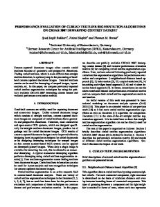
ROC curves provide graphic comparisons of the Az and partial Az measures from Table 2. All ROC plots and analysis shown are based upon the nonparametric empirical data. For the three trials, ROC curves are shown in Figure 1 and partial ROC curves for sensitivity greater than 90%, in Figure 2. The two-tailed p values for intertrial pairwise comparisons of Az and partial Az are shown in Table 3, with significant differences (p < 0.05) highlighted in boldface. These results show certain interesting trends. First, considering only the overall ROC curves in Figure 1, trial A was best, followed by trial C and then trial B. The Az comparisons confirmed this trend. The best trial A and intermediate trial C both had significantly better Az than the worst trial B (p = 0.017 and 0.034, respectively). The best trial A was not significantly better than the intermediate trial C (p = 0.18). This finding was consistent with the two curves being intertwined for a sensitivity of less than 0.80. Second, in comparing the partial ROC curves in Figure 2, the three trials were still rank ordered the same way, with trial A being the best, but trials C and B were much closer to each other. The statistical comparisons of the partial Az measures in Table 3 again confirmed these trends. Trial A was clearly much better than trials B or C (p < 0.001 for both comparisons). The overlapping partial ROC curves for trials B and C were not significantly different from each other (p = 0.46). Because trials B and C were compared at the same fixed 96% sensitivity, it was also possible to compare the specificity, and like the partial Az, this difference was not significant (p = 0.44). Results for the three trials were also analyzed using histogram plots. In the Duke-only trial A, the computer model was optimized using 11 inputs, 10 hidden nodes, and 100 training iterations. Figure 3 depicts a partial histogram plot of the model’s output values. The histogram spanned only the low-end range of values from 0 to 0.28, corresponding

459

Lo et al. to 90% sensitivity or better for this trial. The histogram was dominated by benign cases, indicating the model correctly assigned output values near zero to many benign cases. When a threshold value of 0.10 was applied to this histogram, three malignant cases fell below the threshold (false-negative findings), resulting in 171 true-positive findings of 174 cancers above the threshold or 98% sensitivity, while

potentially obviating 117 of 326 benign biopsies below the threshold or 36% specificity. Note that the value of this threshold depended on the behavior of just a few cancers at the lowest extreme of the histogram. For trial B, all model parameters including the threshold value of 0.10 were fixed to be the same as those in trial A. The resulting partial histogram of trial B is shown in Figure 4, again

Fig. 1.—Graph shows receiver operating characteristic (ROC) curves for three trials, which differ according to whether each was trained or tested on Duke or Penn data sets. Partial ROC plot corresponding to top 10% of this plot is shown in Figure 2. Top line = trial A (Duke/Duke), middle line = trial C (Penn/Penn), bottom line = trial B (Duke/Penn).

Fig. 3.—Partial histogram of model outputs for Duke-only trial A. This model was trained and tested on Duke set. This histogram spans only output range 0–0.284, corresponding to 90% sensitivity or better. Threshold of 0.10 yields 98% sensitivity and 36% specificity as reported in Table 2. White bar = benign, black bar = malignant.

460

only covering the range of values corresponding to 90% sensitivity or better. The model in trial C was optimized just for the Penn cases to establish the upper limit of performance over these cases. This new Penn-only model had the same 11 inputs as before but was optimized at 15 hidden nodes and 200 training iterations. A threshold was applied to the outputs at 0.21 to yield 96%

Fig. 2.—Graph shows partial receiver operating characteristic (ROC) curves (sensitivity ≥ 90%) for three trials. Letters A, B, and C in this plot mark actual operating points used for those trials. Trial A (Duke/Duke) was best performer, followed by closely intertwined curves for trials C (Penn/Penn) and B (Duke/Penn).

Fig. 4.—Partial histogram of model outputs for cross-institutional trial B. This model was trained on the Duke set and tested using the Penn set. Histogram spans only output range 0–0.176, corresponding to 90% sensitivity or better. Applying trial A’s threshold of 0.10 resulted in 96% sensitivity and 28% specificity. White bar = benign, black bar = malignant.

AJR:178, February 2002

BI-RADS Predictive Model for Mammography sensitivity and thus permitted direct comparison with trial B.

Discussion

The BI-RADS lexicon was designed to improve the consistency and accuracy of mammographic reporting. BI-RADS has also been used by computer-aided diagnostic techniques that use the morphology descriptors to identify a subset of currently biopsied lesions that are very likely benign. It was hypothesized that because the computer model was based on standardized input findings, it may be robust enough to generalize to patient data interpreted by different radiologists from different institutions. This study tested that hypothesis by evaluating the model on a large, independent data set from another institution. This challenge was unusual, because most, if not all, computer-aided diagnostic studies to date have been based on training and testing subsets drawn from relatively small local data sets. To evaluate the performance of these models, several different measures were used in this study. The familiar ROC area index, Az, reflected the performance over all possible thresholds applied to the outputs. Two other measures were also reported, however, because of their greater clinical relevance. These were the specificity at a given nearly perfect sensitivity and the partial Az,which was equivalent to the average specificity for all sensitivities above 90%. For a nearly perfect sensitivity such as 98%, the 2% of missed or false-negative findings of cancer would result in delayed diagnosis until the short-term follow-up examination. Previous studies showed that delayed diagnosis of “probably benign” cancers have a minimal impact on the treatment of those cancers [13]. Further study is warranted to assess whether delayed diagnosis for the cases identified by the computer models as very likely benign would have a similarly minimal impact. As shown in the histogram plots, these models generated continuous output values, which may be thresholded to provide binary predictions. Cases with values less than the cutoff threshold would be considered negatives (very likely benign lesions, which may be followed up), whereas those exceeding the threshold would be considered positives (suspicious for malignancy and should be biopsied as before). Reducing the threshold value would detect more cancers (increased sensitivity) but spare fewer benign biopsies (decreased specificity). For a predictive model to generalize to cases it has not seen before, those new cases must be

AJR:178, February 2002

similar to the ones used for training the model. This rule is true whether the model is being applied to new data from the same institution or from a different institution. In this context, “similar” would connote a reasonably comparable patient population in terms of the frequencies and distributions of the input findings and biopsy outcomes. In addition, the radiologists would have to be reasonably consistent in their application of BI-RADS. A certain amount of variability in both factors is inevitable and perhaps even desirable because in practice, a model must work reasonably well at many different institutions under less than perfectly controlled conditions. The data sets from the two different institutions used in this study were compared in Table 1. The mean age, range in ages, and proportion of mass cases were all comparable. Because age and mass margin were previously identified to be two of the most important findings used by the model [21], these provided some assurance that the model may generalize. There were, however, some potentially important differences. Most notably, the Penn cases had a higher proportion of calcification cases (47% vs 38%), which are much more difficult than mass cases to classify for computer models and radiologists alike (Markey MK et al., presented at Chicago 2000: World Congress on Medical Physics and Biomedical Engineering meeting, July 2000). This factor would tend to result in lower model performances in the Penn cases. The Duke and Penn data sets resulted from unrelated projects at each institution. As such, it was not possible to coordinate the data collection procedures nor to retrain the radiologists to control for the effects of interobserver or interinstitutional variability in practice. Fortunately, most important factors were already shared in common between the two sites, namely the use of the BI-RADS lexicon, radiologists at two major academic hospitals with similar levels of expertise, and relatively large biopsy-proven data sets collected over many years to represent each institution’s patient population as closely as possible. The result was two independent data sets, which in turn allowed realistic cross-institutional tests of the model’s performance. Three separate trials were undertaken. Trial A consisted of the existing Duke-only model, which was trained and tested over the 500 Duke cases. Trial B was the interinstitutional evaluation, whereby the above model trained on Duke cases was evaluated using the 1,000 Penn cases. Trial C was the Penn-

only model, trained and tested using the 1,000 Penn cases. If the models generalized perfectly, there would be no differences in performance across the three trials. In other words, the Duke-only model would perform just as well using the Penn data set, as would a new model customized specifically for that Penn data. In practice, however, it was anticipated that differences in the data sets would cause the models to lose some ability to generalize across the three trials. In fact, there was no guarantee that the models would generalize at all in this cross-institutional challenge. The model generalized fairly well, as shown by the performance measures in Table 2. For some loss in sensitivity (96–98%), all models potentially improved specificity considerably (28–36%). Recall that the original clinical decision to recommend biopsy was by definition 100% sensitivity and 0% specificity. Although the cross-institutional trial B was the worst of the three trials, its performance was still reasonably good considering that this was a blinded test using new cases from a different institution. The Penn-only trial C further showed that a separate model could indeed be developed for this independent data set. In other words, the ability to predict breast lesions as benign or malignant using BI-RADS findings was not unique to Duke patient cases interpreted by Duke radiologists. In practice, it would be impractical to collect cases and customize new models for each new institution, but trial C at least confirmed that such an artificial neural network modeling approach has the potential to work at other institutions. Many of the performance differences in our study were, however, statistically significant, as shown in Table 3. This result was especially true for the first comparison of trials A and B, which addressed the crucial question of how well the Duke-only model could generalize to the Penn data set. All measures of performance decreased, and those differences were statistically significant for both Az and partial Az ( p < 0.001 for both). Because the output threshold value was fixed for cross-institutional testing, two of the three trial comparisons (A against B, and A against C) involved operating points with different sensitivity and specificity levels. The usual statistical analysis for a fixed sensitivity or specificity could not be undertaken. Moreover, at such nearly perfect sensitivities, performance depends on a small number of cancers for which the model generated extremely low output values, as shown by the histograms in

461

Lo et al. Figures 3 and 4. With those caveats in mind, the decrease in sensitivity from trial A (98%) to trial B or C (96%) may be evaluated using Poisson counting statistics. For trial B, the cutoff threshold resulted in 18 missed cancers or false-negative results. Assuming these follow a Poisson distribution (mean equals variance), there were 18 ± 4.2 false-negative results, corresponding to 96% ± 1% sensitivity. The 95% confidence interval for trial B’s sensitivity was accordingly [94%, 98%]. Because the mean sensitivity of trial A (98%) lay on the boundary of that confidence interval, the difference was not significant, or at best, barely significant. The uncertainty was calculated for trial B and compared with the mean of trial A instead of the other way around because there were a reasonable number of false-negative results in trial B compared with just three false-negative results in trial A, and the retesting in all cases in trial B avoided any potential bias from round robin sampling in trial A. The Poisson analysis reveals these relatively large data sets of 500 or 1,000 cases may still not be large enough when performance is analyzed at nearly perfect sensitivity. For example, trial A has only three false-negative cases, so to assess the uncertainties associated with its 98% sensitivity, the Duke data set should be more than tripled to yield 10 cases for a good Poisson fit. Even then, the uncertainty would be rather large at 10 ± 3.2 false-negative cases. Ongoing data collection efforts will greatly increase the size of the Duke data set and will facilitate this type of analysis in the future. The cross-institutional evaluation would not be complete without some consideration of the inherent difficulty level of the other data set. The Penn-only trial C was designed to address that issue by establishing the upper bound in performance one could achieve by customizing a new model specifically over these Penn cases. Given the inherent differences in the data sets, the comparison between trials B and C is arguably fairer than that in trials A and B. Trial B was still worse than the standard set by trial C across every performance measure in Table 2. The difference in Az was statistically significant (p = 0.034), although there were no significant differences for the more clinically relevant measures of partial Az ( p = 0.46) or specificity (p = 0.44). This finding was encouraging because the cross-institutional trial did indeed approach its upper limit of performance, at least in the important high sensitivity portion of the ROC curve.

462

In the final comparison of trials A and C in Table 3, the cross-institutional model was taken out of consideration entirely. Instead, the comparison pitted the Duke-only model against the Penn-only model, and any differences would be solely due to a computer model’s ability to characterize each data set. Table 2 shows that trial C was worse than trial A across all performance measures. The Penn data set was inherently more challenging, at least for this type of computer model, probably because of the differences in the data described previously. The differences in Table 3 were significant for partial Az ( p < 0.001) but not Az ( p = 0.18). The former significant difference could account for the similar significant difference between partial Az of trials A and B (p < 0.001) because the cross-institutional model is unlikely to outperform the reoptimized Pennonly model. Unlike simpler diagnostic criteria that provide a fixed binary decision, artificial neural network models take into consideration complex nonlinear interactions between all the input findings and generate a continuous predictive value. The model’s output values were thresholded at 98% sensitivity for trial A and 96% sensitivity for trials B and C. These thresholds may be adjusted to achieve a desired trade-off between sensitivity and specificity. For example, this flexibility may allow the model to perform at a level deemed optimal as a result of cost-effectiveness analysis, simply by adjusting the threshold value up or down. In conclusion, our study investigated some of the challenges in a cross-institutional evaluation of a computer-aided diagnostic model. The models performed well overall, but there were decreases across all measures of performance, with many of those differences statistically significant. These results were, nevertheless, encouraging in two important ways. First, the common use of the standardized BI-RADS lexicon did facilitate one of the first applications of a computer prediction model for breast cancer to a large independent data set from another institution. Second, in the crucial high-sensitivity portion of the ROC curve, the cross-institutional model approached the upper limit of performance set by inherent differences in the two data sets. Clearly there is need for further work to improve the robustness of these models. Ongoing efforts are underway to develop better models using a much larger data set from this institution and mixtures of cases from multiple institutions. Alternative modeling techniques that may yield better generalization of performance

are also being explored. The long-term goal of this work is to develop a model robust enough to generalize to large data sets from all institutions that have similar patient populations and that use the BI-RADS standard. Acknowledgments

We thank all the breast imaging radiologists at both Duke and Penn for their considerable data collection efforts over many years, under the leadership of current and former section heads of breast imaging: Mary Scott Soo and Phyllis Kornguth at Duke and Emily Conant and Daniel Sullivan at Penn. In particular, Daniel Sullivan helped to provide us with the Penn data set. We thank David Delong at Duke and Charles Metz at the University of Chicago for many consultations regarding statistical analysis. We also thank programmer Brian Harrawood and data technicians Käthe Douglas and Beth Winslow.

References 1. Kopans DB. The positive predictive value of mammography. AJR 1992;158:521–526 2. Knutzen AM, Gisvold JJ. Likelihood of malignant disease for various categories of mammographically detected, nonpalpable breast lesions. In: Mayo Clin Proc 1993;68:454–460 3. Cyrlak D. Induced costs of low-cost screening mammography. Radiology 1988;168:661–663 4. Zheng B, Chang YH, Wang XH, Good WF, Gur D. Feature selection for computerized mass detection in digitized mammograms by using a genetic algorithm. Acad Radiol 1999;6:327–332 5. Qian W, Clarke LP, Song D, Clark RA. Digital mammography: hybrid four-channel wavelet transform for microcalcification segmentation. Acad Radiol 1998;5:354–364 6. Qian W, Li L, Clarke L, Clark RA, Thomas J. Digital mammography: comparison of adaptive and nonadaptive CAD methods for mass detection. Acad Radiol 1999;6:471–480 7. Chan HP, Sahiner B, Helvie MA, et al. Improvement of radiologists’ characterization of mammographic masses by using computer-aided diagnosis: an ROC study. Radiology 1999;212:817–827 8. Chan HP, Sahiner B, Lam KL, et al. Computerized analysis of mammographic microcalcifications in morphological and texture feature spaces. Med Phys 1998;25:2007–2019 9. Jiang Y, Nishikawa RM, Schmidt RA, Metz CE, Giger ML, Doi K. Improving breast cancer diagnosis with computer-aided diagnosis. Acad Radiol 1999;6:22–33 10. Huo Z, Giger ML, Vyborny CJ, Wolverton DE, Schmidt RA, Doi K. Automated computerized classification of malignant and benign masses on

AJR:178, February 2002

BI-RADS Predictive Model for Mammography digitized mammograms. Acad Radiol 1998;5: 155–168 11. Baker JA, Kornguth PJ, Lo JY, Williford ME, Floyd CE Jr. Breast cancer: prediction with artificial neural network based on BI-RADS standardized lexicon. Radiology 1995;196:817–822 12. Lo JY, Baker JA, Kornguth PJ, Floyd CE Jr. Effect of patient history data on the prediction of breast cancer from mammographic findings with artificial neural networks. Acad Radiol 1999;6:10–15 13. Sickles EA. Periodic mammographic follow-up of probably benign lesions: results in 3,184 consecutive cases. Radiology 1991;179:463–468

14. American College of Radiology. Breast imaging reporting and data system (BI-RADS), 3rd ed. Reston, VA: American College of Radiology, 1998 15. Kopans DB. Standardized mammography reporting. Radiol Clin North Am 1992;30:257–264 16. D’Orsi CJ, Kopans DB. Mammographic feature analysis. Semin Roentgenol 1993;28:204–230 17. Baker JA, Kornguth PJ, Lo JY, Floyd CE Jr. Artificial neural network: improving the quality of breast biopsy recommendations. Radiology 1996; 198:131–135 18. Jiang Y, Metz CE, Nishikawa RM. A receiver op-

erating characteristic partial area index for highly sensitive diagnostic tests. Radiology 1996;201: 745–750 19. Efron B. The Jackknife, the bootstrap and other resampling plans. Philadelphia: Society for Industrial and Applied Mathematics, 1982:92 20. Efron B, Tibshirani RJ. An introduction to the bootstrap. New York: Chapman & Hall, 1993:436 21 Lo JY, Baker JA, Kornguth PJ, Floyd CE Jr. Computer-aided diagnosis of breast cancer: artificial neural network approach for optimized merging of mammographic features. Acad Radiol 1995;2: 841–850

ARRS 2002 Annual Meeting Symposium focuses on breast cancer screening. Experts will present the latest information on the various screening methods, including digital mammography, sonography, and MR imaging. Screening economics and medicolegal issues will also be discussed. The Annual Meeting will be held April 28-May 3 in Atlanta. Log on to www.arrs.org for further information.

AJR:178, February 2002

463