1
CT reconstruction from parallel and fan-beam projections by 2D discrete Radon transform Amir Averbuch, Ilya Sedelnikov and Y. Shkolnisky
Abstract—The Discrete Radon transform (DRT) was defined in [5] as an analogue of the continuous Radon transform for discrete data. Both the DRT and its inverse are computable in O(n2 log n) operations for images of size n×n. In this paper, we demonstrate the applicability of the inverse DRT for the reconstruction of a 2D object from its continuous projections. The DRT and its inverse are shown to accurately model the continuum as the number of samples increases. Numerical results for the reconstruction from parallel projections are presented. We also show that the inverse DRT can be used for reconstruction from fan-beam projections with equispaced detectors. Index Terms—Tomography, CT, 2D discrete Radon transform, parallel projections, fan-beam projections.
I. I NTRODUCTION Tomographic reconstruction underlies nearly all diagnostic imaging modalities, including x-ray computed tomography (CT), positron emission tomography, single photon emission tomography and certain acquisition methods for magnetic resonance imaging. It is also widely used for nondestructive evaluation in manufacturing and more recently for airport baggage security. Reconstruction in tomography means a recovery (inversion) from samples of either the x-ray transform (set of line-integral projections) or the Radon transform (set of integrals on planes) of an unknown object density distribution. In the 2D case, they are the same. In the 2D case, the Radon transform of a function f (x, y), denoted by
−∞
(I.1) where δ(x) is Dirac’s delta function [1], [3]. In CT imaging, f (x, y) is the distribution of the x-ray attenuation coefficient within the object. The goal of CT imaging is to reconstruct f (x, y) from the projections of the object. Each projection is a collection of line integrals as in Eq. (I.1). Parallel projection and fan-beam projection are two common acquisition geometries. Parallel projection is given by
formed by line integrals along rays that emanate from a single source. Due to physical constraints on the size and the number of detectors, in practice each projection is comprised of a finite number of line integrals. For parallel projections, this means that s ∈ {s1 , . . . , sm } for some finite m. Only finite number of projections can be collected, that is θ ∈ {θ1 , . . . , θn } for some integer n. When a single source of radiation is used, fan-beam projections are more efficient, since all the measurements in one fan are acquired simultaneously. For this reason, commercial CT scanners use fan-beam projections. Computations speedups to recover objects from projections (either parallel or fan-beam) are critical for next-generation real-time imaging systems. Several fast reconstruction algorithms have been proposed. Bresler et. al. [7], [9] uses fast hierarchical algorithms for tomographic reconstruction where filtered backprojection (FBP) is the reconstruction method. The straightforward approach, which utilizes FBP, has a computational bottleneck of complexity O(n3 ) operatins for a 2D n × n image and at least O(n4 ) operations for a 3D n × n × n image. A family of fast hierarchical tomographic backprojection algorithms, which reduce the complexity to O(n2 log n) for the 2D case, was presented in [7], [9]. The algorithm employs a divide-and-conquer strategy in the image domain and relies on properties of harmonic decomposition of the Radon transform. For typical image sizes in medical applications or airport baggage security, these computations speeds-up by more than an order of magnitude. This algorithm is an accelerated version of the standard filtered backprojection (FBP) reconstruction for parallel beam tomography. It provides orders of magnitude speedup in reconstruction time with little or no added distortion. Other fast reconstruction algorithms, which exhibit O(n2 log n) complexity, have been proposed. They include what is known collectively as Fourier reconstruction algorithms (FRA) and multilevel inversion (MI) algorithms. FRA are based on the Fourier Slice Theorem [2], which states that the Fourier transform of a projection at angle θ is a radial slice through the 2D Fourier transform of the object at direction θ. Before the appearance of our algorithms [4], [5], on which the new algorithms in this paper are based, Fourier reconstruction algorithms have been formed by the following sequence of steps: 1) FFT is applied to the padded projections; 2) A 2D Cartesian FFT grid is interpolated from the polar grid; 3) The image is recovered by a 2D Inverse FFT.
2
The difficulty lies in step 2. The interpolation step introduces distortions in the reconstruction, since the Fourier transform is sensitive to these interpolations. The gridding method in [13] for the reconstruction was used in [7] for comparison with their performance. According to [7], their algorithm outperforms the Fourier based reconstruction algorithms [13] and the multilevel inversion algorithm in [6]. Both have O(n2 log n) complexity. The proposed hierarchical scheme has a superior cost versus distortion performance as suggested in [7]. A model for finite Radon transforms that is composed of Radon projections is presented in [14]. They do not interpolate between points, but they perform summation over lines with “wraparound”. In some disctretizations, “wraparound” is inherent and this is a major drawback, since algorithms, which are based on summation along wrapped lines, cannot be used for reconstruction from continuous projections (see Theorem II.2). The proposed algorithms in this paper are simpler than those in [7]. In fact, they can be implemented using only 1D FFTs. The underlying transforms for these algorithms are proven in [4], [5] to be algebraically accurate, preserve the geometric properties of the continuous transforms, invertible and rapidly computable. In addition, it is shown in [5] that the discrete Radon transform converges to the continuous Radon transform, as the discretization step goes to zero. This property is of major theoretical and computational importance since it shows that the discrete transform indeed approximates the continuous transform, and thus it can be used to replace the continuous transform in digital implementations. The Equally-Sloped Tomography (EST) method introduced in [10] is an iterative one which allows reconstructions from a limited number of noisy projections ([11], [12]) through the a use of total-variation regularization. The use of regularization also allows for reduction of aliasing artifacts which originated from incorrect sampling (e.g. inaccessible information beyond the resolution circle, see [10], [11]). These works extend innovatively the pseudo-polar representation ([4], [5]) on which we based our algorithm to overcome the problem of reconstruction from a limited number of noisy projections when for example dose reduction is requested. When projection data, which was collected along the lines for which direct Radon transform is defined (where the distance between lines depends on the angle), is translated to Fourier domain by means of 1D Fourier of each projection, then the resulting data lies on the pseudo-polar gird points and not on the polar grid. Therefore, the ’resolution circle’ problem does not exist due to the different acquisition geometry (distance between lines depends on the acquisition angle). In this paper, multiple samples per detector width and different acquisition geometry are described in section IV, which together eliminates the resolution circle problem. Then, Radon transform reconstruction is preferable for two reasons: 1. As shown in section III, correctly sampled projection reconstruction exhibits virtually no visible artifacts apart of a smoothing caused by the aperture function. In the situation when aliasing artifacts are not prominent, there is no added value in using the EST regularization. 2. Inverse Radon
transform is faster than iterative procedure used in EST. When the projection data contains aliased information (incorrectly sampled) inverse Radon will exhibit reconstruction artifacts. In these cases, regularization used in EST has an advantage over formal inverse Radon since it reduces aliasing artifacts. When the collection procedure is designed such that the signal is band limited prior to sampling (aperture function) and the sampling rate is increased (multiple samples per detector width), then the severity of the aliasing problem decreases no matter if the ’resolution circle’ problem is present or not, due to the fact that the sampled signal becomes essentially band limited. The reconstruction examples presented in this paper are based on projections which satisfy both requirements. The structure of the paper is as follows. Section II shortly describes the discrete Radon transform [5] together with the results and properties that are relevant to the proposed algorithms. Section III demonstrates a reconstruction from samples of the continuous Radon transform, which is the basis for the reconstruction from fan-beam projections. Finally, in Section IV, we describe reconstruction from fan-beam projections, including the acquisition geometry and the “re-sorting” algorithm which is the basis for the presented algorithm.
II. 2D DISCRETE R ADON TRANSFORM A 2D discrete Radon transform is defined in [5] as an analogue of the continuous Radon transform for discrete images. Generally speaking, the discrete Radon transform is defined by summing the discrete samples of the image I(u, v) along lines with absolute slope less than 1. We define two families of lines: 1. basically horizontal line is a line of the form y = sx + t where |s| ≤ 1. 2. basically vertical line is a line of the form x = sy + t where |s| ≤ 1. For basically horizontal lines, we traverse each line by unit horizontal steps x = −n/2, . . . , n/2 − 1, and for each x, we interpolate the image sample at position (x, y) by using trigonometric interpolation along the corresponding image column. For basically horizontal lines we traverse the line by unit vertical steps, and for each integer y, we interpolate the value at the x coordinate x = s0 y + t0 by using trigonometric interpolation along the corresponding row. A formal definition of a 2D radon transform from [5] is provided below: Definition II.1 ([5] 2D Radon transform for discrete images). Let I(u, v), u, v = −n/2, . . . , n/2 − 1, be a n × n array. Let s be a slope such that |s| ≤ 1, and let t be an intercept such that t = −n, . . . , n. Then, n/2−1
Radon({y = sx + t}, I) =
X
Ie1 (u, su + t),
(II.1)
Ie2 (sv + t, v),
(II.2)
u=−n/2 n/2−1
Radon({x = sy + t}, I) =
X
v=−n/2
3
where for u, v = −n/2, . . . , n/2 − 1, x, y ∈ R n/2−1
Ie1 (u, y) =
X
I(u, v)Dm (y − v),
(II.3)
I(u, v)Dm (x − u),
(II.4)
v=−n/2 n/2−1
Ie2 (x, v) =
X
u=−n/2
and Dm (t) =
sin(πt) , m sin (πt/m)
m = 2n + 1.
(II.5)
Moreover, for an arbitrary line l with slope s and intercept t, such that |s| ≤ 1 and t = −n, . . . , n, the Radon transform is given by (RI)(s, t) = ½ Radon({y = sx + t}, I) l is a basically horizontal line Radon({x = sy + t}, I) l is a basically vertical line. (II.6) The 2D discrete definition of the Radon transform is shown in [5] to be geometrically faithful as the lines used for the summation exhibit no wraparound effects. We also show that it satisfies a Fourier slice theorem, which states that the 1D Fourier transform of the discrete Radon transform is equal to the samples of the pseudo-polar Fourier transform of the underlying image that lie along a ray. There exists a special set of parallel projections for which the transform is rapidly computable and invertible. For a discrete image I(u, v), u, v ∈ [−n/2 : n/2 − 1], this set consists of n+1 basically horizontal and n+1 basically vertical © ª projections, given© by the setsª SH (t, l) = y = 2l nx+t n n and SV (t, l) = x = 2l n y + t , where l ∈ [− 2 : 2 ] and t ∈ [−n : n]. For a fixed l ∈ [− n2 : n2 ], the l-th basically horizontal projection is composed of summations along lines from the ¯ ¯ 2l set SH (·, l) = {y = n x + t ¯t ∈ [−n : n]}. The l-th basically vertical projection is composed of¯ summations along lines ¯ from the set SV (·, l) = {x = 2l n y+t ¯t ∈ [−n : n]}. We denote the results from these discrete summations by PH (t, l) = Radon(SH (t, l), I) and PV (t, l) = Radon(SV (t, l), I), l ∈ [− n2 : n2 ] and t ∈ [−n : n]. The discrete Radon transform [5] has both forward and inverse algorithms with complexity O(n2 log n) for images of size n × n. We briefly describe the inversion algorithms, as they are the main ingredient of the proposed reconstruction procedure. There are two inversion approaches, namely, an iterative and a direct. In both cases, we use the discrete version of the Fourier slice theorem [5] to transform the problem from the Radon domain into the Fourier domain, thus formulating the reconstruction problem as the inversion of a non-uniform Fourier transform on a certain non-uniform grid. The resulting frequency grid is the so-called pseudo-polar grid [4]. The iterative algorithm is based on the application of the conjugate-gradient method to the Gram operator of the pseudopolar Fourier transform. Since both the forward pseudopolar Fourier transform and its adjoint can be computed in O(n2 log n) operations, where n × n is the size of the input
image, the Gram operator can also be computed in the same complexity. More specifically, both the pseudo-polar Fourier transform and its adjoint can be computed using 100n2 log n operations plus small lower order terms [4] p.771. This sums to 200n2 log n operations per iteration. For comparison, the 2D FFT of a n × n image requires 10n2 log n operations. The number of iterations is shown in [4] to be small for any practical image size (less than 6 iterations). The advantage of the iterative inversion algorithm is its simplicity. On the other hand, it does not utilize the special frequency domain structure of the transform and its execution time depends on the specific image to invert. Thus, [4] provides also a direct inversion algorithm, which directly resamples the pseudo-polar grid to a Cartesian frequency grid and then, recovers the image from the Cartesian frequency grid. The algorithm is based on an “onion-peeling” procedure that at each step recovers two rows/columns of the Cartesian frequency grid, from the outermost rows/columns to the origin, by using columns/rows recovered in previous steps. The Cartesian samples of each row/column are recovered using trigonometric interpolation that is based on a Fast Multipole Method (FMM). Finally, the original image is recovered from the Cartesian frequency samples, which are not the standard DFT samples, by using a fast Toeplitz solver. Full details on both algorithms are given in [4]. We prove in [5] that if the image I(u, v) consists of samples of the function f (x, y) on a Cartesian grid, then the 2D discrete Radon transform of I(u, v) approximates the continuous parallel projections of f (x, y). Rephrasing the convergence theorem in [5], we have the following result: Theorem II.2. ([5]) Assume f (x, y) ∈ Lipα (R) 1 that equals to zero outside the square (−1 + ε, 1 + ε) × (−1 + ε, 1 − ε) for some ε > 0. Define In (u, v) = f (u n2 , v n2 ), n ∈ N,. Then, for n → ∞ ¯ ¯ Z ∞ ¯ ¯ 2l 2 2l 2t ¯ ¯ f (x, x+ )dx¯ −→ 0 ¯Radon({y = x+t}, In )· − ¯ ¯ n n −∞ n n and ¯ ¯ Z ∞ ¯ ¯ 2 2l 2t 2l ¯ ¯ f ( y+ , y)dy ¯ −→ 0 ¯Radon({x = y+t}, In )· − ¯ ¯ n n n n −∞ uniformly for l ∈ [− n2 :
n 2]
and t ∈ [−n : n].
In order to establish a correspondence between discrete projections and samples of continuous projections we define R∞ two families of line integrals L (α, β) = f (x, αx+β)dx H −∞ R∞ and LV (α, β) = −∞ f (αy +β, y)dy. For a fixed α ∈ [−1, 1], the function LH (α, β), which is viewed as a function of β, is a continuous projection of f (x, y) along the vector (1, α), where β is an intercept of the corresponding ray with the yaxis. For a fixed α ∈ [−1, 1], the function LV (α, β), which is viewed as a function of β, is a continuous projection of f (x, y) along the vector (α, 1), where β is an intercept of the 1 Lipschitz class Lip (α, Ω): Let Ω ⊆ Rn . If f : Rn → C satisfies the C condition |f (x) − f (y)| ≤ Ckx − ykα , 0 < α ≤ 1 for all x, y ∈ Ω, then we say that f belongs to the class LipC (α, Ω). When the value of the constant C is not important we say that f is Lipschitz α on Ω.
4
n Error
64 0.1803
128 0.0892
256 0.0461
512 0.0223
1024 0.0117
TABLE II.1: Relative l2 error between the analytic computation and the approximated projections.
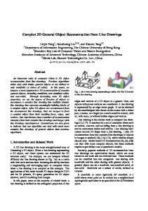
corresponding ray with the x-axis. By analogy with SH and SV in the discrete domain, we e define two sets ªof lines in the continuous domain © © ª SH (t, l) = 2l 2 2l 2 e y = n x + n t and SV (t, l) = x = n y + n t , where l ∈ [− n2 : n2 ] and t ∈ [−n : n]. e We ¡ denote ¢ line integrals along ¡ these¢ lines by PH (t, l) = 2t eV (t, l) = LV 2l , 2t , where l ∈ [− n : n ] LH 2l , and P n n n n 2 2 and t ∈ [−n : n]. In fact, PeH (t, l) is composed of sampled continuous parallel projections. Indeed, for a fixed l from [− n2 : n2 ], the e vector of samples of continuous projection ¡ 2l PH¢(t, l) consists LH n , β at points 2t n for t ∈ [−n : n]. Similar statement is true for PeV (t, l). By Theorem II.2, PH (t, l) · n2 converges to PeH (t, l) and PV (t, l) · n2 converges to PeV (t, l) as n grows. Theorem II.2 is illustrated by comparing between the discrete and the sampled continuous projections of the SheppLogan head phantom. The density function f (x, y) of the Shepp-Logan phantom is a sum of indicator functions of ellipses weighted by the density of each ellipse. The function f (x, y) equals zero outside the square [−1, 1] × [−1, 1]. The advantage of the Shepp-Logan phantom is that an analytic expression for its projections can be derived. The full range of densities in the Shepp-Logan phantom is [0, 1], which is equivalent to the range of [0, 1000] in Hounsfield units (HU). The Shepp-Logan head phantom is displayed in (Fig. II.1) with a window-width of 100 HU centered about water. Notice that the Shepp-Logan phantom is not a Lipschitz function. Therefore, it violates the conditions of Theorem II.2. Nonetheless, the discrete projections of the phantom closely approximate the continuous sampling, as we will see below. Consider a discrete image I(u, v) = f (u n2 , v n2 ), u, v ∈ [− n2 , n2 − 1], for some positive integer n. We compute the 2D discrete Radon transform for this image, which results in the two projections arrays PH and PV . We multiply both arrays by n2 to approximate the sampled continuous projections. The scaled arrays for the case n = 512 are displayed in Fig. II.2a. We then compute the two arrays PeH and PeV of sampled continuous projections of f (x, y) (see Fig. II.2b for illustration). It follows from Theorem II.2 that the entries in PH and PV approximate the entries in PeH and PeV . In our example, the computed relative l2 error between the arrays in Figs. II.2a and II.2b equals 0.0223. Absolute error is shown in Fig. II.2c. Table II.1 shows the relative l2 errors between the samples of the analytic computation and the approximated projections of the Shepp-Logan phantom for different values of n. We observe that in the case of the Shepp-Logan phantom, the relative l2 error is proportional to n1 . Another way to estimate the quality of the approximations is to compute the relative l2 error separately for each projection. Figure II.3 displays graphs of the error as a function of the
projection index l ∈ [−n/2 : n/2] for n = 512. Convergence of the discrete projections to sampled continuous projections implies that we can reconstruct f (x, y) from its continuous projections by applying the 2D inverse discrete Radon transform. III. R ECONSTRUCTION FROM PARALLEL CONTINUOUS PROJECTIONS
In this section, we provide numerical evidence that the inverse discrete Radon transform can be used for reconstruction from sampled x-ray projections. The numerical examples are based on analytically computed parallel projections of the Shepp-Logan phantom. Let f (x, y) denotes the continuous Shepp-Logan phantom and let n be a fixed integer number. Arrays PeH (t, l) and PeV (t, l), which were defined in Section II, are composed from samples of analytic projections of the Shepp-Logan phantom. We apply the 2D inverse Radon transform to PeH (t, l) · n2 and to PeV (t, l) · n2 , obtaining an n × n image which approximates the original phantom f (x, y) sampled at the points {(u n2 , v n2 ) | u, v ∈ [− n2 : n2 − 1]}. However, since the analytic projections of the Shepp-Logan phantom are not bandlimited, the resulting image will suffer from aliasing artifacts. We provide an example of such a reconstruction for n = 512 in Fig. III.1a. Reconstructed image is displayed using window-width of 100 HU that is centered around water. The difference between the samples of the Shepp-Logan phantom and the reconstructed image is displayed in Fig. III.1b using window-width of 50 HU. In practice, x-ray projections are always bandlimited due to the non-zero size of the detector aperture of the x-ray source. We simulate the non-zero detector aperture by convolving the analytic projections with an aperture function prior to sampling. We define LσH (α, β) = LH (α, β) ∗ Πσ (β) and LσH (α, β) = LV (α, β) ∗ Πσ (β) where the sensor aperture is simulated using convolution with a rectangular function ½ 1 β ∈ {−σ, σ} 2σ Πσ (β) = (III.1) 0 otherwise. σ should satisfy σ ≥ Ts in order to reduce aliasing, where Ts is a center-to-center distance between sensors - see [3] p.188. This inequality means that there should be at least two samples per detector width. There exists a number of ways to measure multiple samples per detector width in practice, see for example [3] pp.188-189. In our simulation, Ts = 2/n which is the distance between subsequent samples on the receiver line. We sample the continuous projections convolved ¢ the ¡ with 2t σ , and aperture function to obtain PeH (t, l) = LσH 2l n n ¡ ¢ n n σ σ 2l 2t e PV (t, l) = LV n , n , where l ∈ [− 2 : 2 ] and t ∈ [−n : n]. σ We then apply the 2D inverse Radon transform to PeH (t, l) · n2 n σ and PeV (t, l) · 2 in order to obtain n × n image which approximates of the original phantom f (x, y) that is sampled at the points {(u n2 , v n2 ) | u, v ∈ [− n2 : n2 − 1]}. The resulting reconstruction for n = 512 and σ = 2/n is displayed in Fig. III.2. Aliasing artifacts are significantly reduced as compared to Fig. III.1.
5
Original phantom 0.05 50
0.04
100
0.03
150
0.02
200
0.01
250
0
300
−0.01
350
−0.02
400
−0.03
450
−0.04
500 0
100
200
300
400
−0.05
500
Fig. II.1: Shepp-Logan head phantom
100
100
100
100
200
200
200
200
300
300
300
300
400
400
400
400
500
500
500
500
600
600
600
600
700
700
700
700
800
800
800
800
900
900
900
900
1000
1000
1000
1000
100
200
300
400
500
100
200
300
400
500
100
200
300
400
500
100
(b) PeH and PeV
(a) PH and PV
100
100
200
200
300
300
400
400
500
500
600
600
700
700
800
800
900
900
1000
1000 100
200
300
400
500
100
200
300
400
500
(c) Absolute error
Fig. II.2: Discrete projections vs. continuous projections.
200
300
400
500
6
l2 error for basically vertical projections
l2 error for basically horizontal projections 0.028 0.026
0.026 0.024 relative l2 error
2
relative l error
0.024
0.022
0.022 0.02
0.02 0.018 0.018
0.016
0.016 0.014 −200
−100
0 projection number
100
200
−200
−100
(a) Basically horizontal
0 projection number
100
200
(b) Basically vertical
Fig. II.3: Relative l2 error as a function of the projection number l.
0.05
0.025
50
0.04
50
0.02
100
0.03
100
0.015
150
0.02
150
0.01
200
0.01
200
0.005
250
0
250
0
300
−0.01
300
−0.005
350
−0.02
350
−0.01
400
−0.03
450
−0.04
500 100
200
300
400
500
−0.05
400
−0.015
450
−0.02
500 100
(a) Recovered Shepp-Logan
200
300
400
500
−0.025
(b) Reconstruction error
Fig. III.1: Reconstruction from PeH and PeV
0.05 50
0.025
0.04
50
0.02
100
0.03
100
0.015
150
0.02
150
0.01
200
0.01
200
0.005
250
0
250
0
300
−0.01
300
−0.005
−0.02
350
−0.01
350 400
−0.03
450
−0.04
500 100
200
300
400
500
−0.05
400
−0.015
450
−0.02
500 100
(a) Recovered Shepp-Logan
Fig. III.2: Reconstruction from
200
300
400
(b) Reconstruction error σ PeH
and PeVσ
500
−0.025
7
50
50
100
100
150
150
200
200
250
250
300
300
350
350
400
400
450
450
500
500 100
200
300
400
500
100
(a) Errors above 0.001
200
300
400
500
(b) Errors above 0.005
50
50
100
100
150
150
200
200
250
250
300
300
350
350
400
400
450
450
500
500 100
200
300
400
500
(c) Errors above 0.01
100
200
300
400
500
(d) Errors above 0.02
σ Fig. III.3: Error masks from the reconstruction from PeH and PeVσ
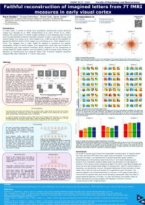
The reconstruction error is visualized by providing binary mask images where a pixel has a white color whenever the absolute reconstruction error is bigger than 1 HU for Fig. III.3a , 5 HU for Fig.III.3b , 10 HU for Fig.III.3c and 20 HU for Fig.III.3c. As can be seen from the images, the reconstruction error is concentrated near and outside the two external ellipses. Internal structures are reconstructed perfectly except of smoothing caused by the non-zero aperture size. Remaining aliasing artifacts are below 10 HU except of some isolated points. We further demonstrate that remaining artifacts are indeed aliasing result rather than reconstruction error of our algorithm. To show this, we use reconstruction from projections which were convolved with the Gaussian function G(x) = 2 1 √ exp(− σx2 ), which has approximately the same smoothing σ π effect on edges as the rectangular function Π(x) but has a more compact representation in the frequency domain. Reconstruction error for n = 512 and σ = n2 is displayed in Fig. III.4a using window-width of 50 HU. The binary mask from the errors above 0.005 is displayed in Fig. III.4b. We observe that the reconstruction error is less than 5 HU everywhere except in the ellipse edges. The error near the edges is a result from smoothing the projections with the aperture function.
Overall, we demonstrated that our algorithm produces good reconstruction quality whenever projections are correctly sampled.
IV. FAN - BEAM RECONSTRUCTION In Section III, we showed that the 2D inverse discrete Radon transform can be used for the reconstruction of an object from its continuous projections along lines from SeH and SeV . Collecting this set of projections by a single pair of source/detector is a time-consuming operation, since for each projection angle, the source/detector pair should scan linearly over the orthogonal direction collecting 2(n+1) line integrals. This process should be repeated for each projection angle. Overall, the source should be turned on and off 2(n+1)(2n+1) times in order to collect the required projections. In this section, we show that if we can afford using multiple detectors with a single radiation source (as is the case with contemporary scanners), we can efficiently collect all the required line projections using certain fan-beam projections. The process, which composes parallel projections from lines that were collected using fan-beam projections, is usually referred to as “re-sorting”.
8
0.025 50
0.02
50
100
0.015
100
150
0.01
150
200
0.005
200
250
0
250
300
−0.005
300
350
−0.01
350
400
400
−0.015
450
450
−0.02
500 100
200
300
400
500
500
−0.025
100
(a) Reconstruction error
200
300
400
500
(b) Errors above 0.005
Fig. III.4: Reconstruction errors from projections smoothed with Gaussian.
line from SeH can be uniquely defined as the line that passes through the two points (−2, n2 z) and (2, n2 w), z, w ∈ [−2n : 2n]. By placing the set of detectors at the points (2, n2 w), w ∈ [−2n : 2n], and successively placing the radiation source at points (−2, n2 z), z ∈ [−2n : 2n], we can collect all the projections from SeH . By swapping axes we can collect in the same way the projections along lines from SeV . Therefore, all the line projections required in order to reconstruct an n × n discrete approximation of f (x, y) using the 2D inverse discrete Radon transform are contained in (4n+1)+(4n+1) = 8n+2 fan-beam projections, where the radiation source moves along a straight line with equal steps. As we mentioned above, each line in SeH can be described either by the parameters (l, t), l ∈ [− n2 : n2 ] and t ∈ [−n, n], or by the pair (z, w), z, w ∈ [−2n : 2n]. In Section IV-B we establish the correspondence between these two representations.
4 3 2 1 0 −1 −2 −3 −4 −2
B. The re-sorting algorithm 0
2
Fig. IV.1: Basically horizontal lines for n = 4.
A. Acquisition geometry We consider a 2D object, described by f (x, y), such that f (x, y) = 0 outside [−1, 1] × [−1, 1]. For n = 4, we draw all the lines from SeH in Fig. IV.1. All the line integrals in this figure can be collected using fan-beam projections with sources on the line x = −2. This is true for any n. Indeed, the y-coordinates of points of intersection with lines from SeH 2 with the vertical line x = −2 are y = − 4l n + n t, which are 2 multiples of n by an integer from [−2n : 2n]. Points of intersection between basically horizontal lines and 2 the vertical line x = 2 are y = − 4l n + n t, which are also 2 multiples of n by an integer from [−2n : 2n]. Therefore, each
Consider a point (−2, n2 z), z ∈ [−2n : 2n]. We want to find which lines from SeH pass through this point. Formally, for each z ∈ [−2n : 2n] we want to find the set ½ ¾ h n ni ¯2 2l 2 Sz = (l, t)¯ z = (−2) + t, l ∈ − : , t ∈ [−n : n] . n n n 2 2 We get n h n ni o ¯ Sz = (l, t)¯z = −2l + t, l ∈ − : , t ∈ [−n : n] . 2 2 If we consider a plane with Cartesian coordinates l and z, then z = −2l+t is a straight line with slope −2 that intersects the z-axis at t. For l ∈ [− n2 , n2 ] and t ∈ [−n, n], the points (l, z) cover a parallelogram with vertices at (− n2 , 2n),(− n2 , 0), ( n2 , 0) and ( n2 , −2n). Therefore, for each z ∈ [0, 2n] there exists t ∈ [−n, n] such that z = −2l + t if and only if l ∈ [− n2 , n−z 2 ]. Similarly, for each z ∈ [−2n, 0] there exists t ∈ [−n, n] such that z = £ ¤ n , −2l + t if and only if l ∈ − n+z . 2 2
9
We now return to the task of finding Sz . We consider four cases, depending on whether z is even or odd and whether z is positive or negative. Theorem IV.1. For z ∈ [−2n : 2n], the set Sz is given by the following formulae: 1) For z = 2k, k ∈ [0 : n] ½ · ¸¾ ¯ n n−z ¯ Sz = (l, z + 2l) ¯ l ∈ − : . 2 2 2) For z = 2k − 1, k ∈ [1 : n] ½ · ¸¾ ¯ n n−z−1 ¯ Sz = (l, z + 2l) ¯ l ∈ − : . 2 2 3) For z = −2k, k ∈ [1 : n] ½ · ¸¾ ¯ −n − z n ¯ Sz = (l, z + 2l) ¯ l ∈ : . 2 2 4) For z = −2k + 1, k ∈ [1 : n] ½ · ¸¾ ¯ −n − z + 1 n ¯ Sz = (l, z + 2l) ¯ l ∈ : . 2 2 Proof: We prove the case z = 2k − 1, k ∈ [1 : n]. It follows from the geometric considerations above that there t ∈ ¤[−n, n] such that z = −2l + t if and only if l ∈ £exists − n2 , n−z , that is l ∈ [− n2 , n2 − k + 12 ]. Since we are looking 2 for an integer l, this is equivalent to l ∈ [− n2 : n2 − k] which is, in turn, equivalent to l ∈ [− n2 : n−z−1 ]. 2 Sincen z = −2l ¯+ t, we have t = o z + 2l. Consequently ¤ £ ¯ . The proofs of the Sz = (l, z + 2l) ¯ l ∈ − n2 : n−z−1 2 other cases are similar. Corollary IV.2. The pair (z, w) defines a line from SeH if and only if z, w ∈ [−2n : 2n] and w = z + 4l for some l ∈ SL (z), where SL (z) is defined as follows: ¤ £ . ¤ 1) If z = 2k, k ∈ [0 : n], then SL (z) = −£n2 : n−z 2 2) If z = 2k −1, k ∈ [1 : n], then SL (z) =£ − n2 : n−z−1 . 2¤ n 3) If z = −2k, k ∈ [1 : n], then SL (z) = −n−z : . 2 2 4) £If z = −2k + 1, k ∈ [1 : n], then SL (z) = ¤ −n−z+1 : n2 . 2 Proof: It follows immediately from Theorem IV.1 and the fact that (z, w) defines some line from SeH if and only if there exist l ∈ [− n2 , n2 ] and t ∈ [−n, n] such that z = −2l + t and w = 2l + t. For each pair (l, t) that defines a line from SeH we can find 2 ( n z, n2 w) as the points of intersection of this line with the vertical lines x = −2 and x = 2. Therefore, 2l (−n) + t = −2l + t n 2l w = (n) + t = 2l + t. n
z=
Vice versa, if the pair (z, w) defines a line from SeH (which we can check using Corollary IV.2), then the parameters (l, t) are w+z w−z t= l= . 2 4 We now describe the algorithm for collecting the set of line
projections PeH (t, l) using fan-beam projections. As usual, we assume that the object under consideration fits within the box [−1, 1] × [−1, 1]. Detectors are placed at the points (2, n2 w), w ∈ [−2n : 2n]. Each fan-beam projection is acquired by placing the radiation source at one of the points (−2, n2 z), where z ∈ [−2n : 2n]. We denote by Pz (w) the output of the detector located at (2, n2 w) when the object is illuminated by the point source located at (−2, n2 z). For a fixed z ∈ [−2n ¯ : ¯ w+z 2n], we set PeH ( w−z , ) = P (w) for all w ∈ {z + 4l ¯l∈ z 4 2 Sz (l)}. The algorithm that collects PeV is identical up to a swap of the axes. It is important to notice here, that we have a choice of either collecting data for all pairs (z, w) and then selecting the pairs that correspond to lines from SeH , or collecting only the necessary projections by discarding the output of detectors for which the line given by (z, w) is not within SeH . Once all the necessary projections are collected we can reconstruct the object using an algorithm of Section III. V. C ONCLUSIONS In this paper, we showed that the inverse DRT can be used for the reconstruction of a 2D object from its continuous projections. The DRT and its inverse are shown to accurately model the continuum as the number of samples increases. Numerical results for the reconstruction from parallel projections are presented. We also show that the inverse DRT can be used for reconstruction from fan-beam projections with equispaced detectors. The Shepp-Logan phantom is not a Lipschitz function and its analytic projections are not bandlimited. Therefore, it violates the conditions of Theorem II.2. Nonetheless, the discrete projections of the phantom closely approximate the sampled continuous ones as was shown in the paper. CT reconstruction from parallel and fan-beam projections for 3D X-Ray data is a natural extension of the 2D case. R EFERENCES [1] S. R. Deans, The Radon Transform and Some of Its Applications, New York: Wiley, 1983. [2] F. Natterer, The Mathematics of Computerized Tomography. New York: Wiley, 1986. [3] A. Kak and M. Slaney, Principles of Computerized Tomographic Imaging, New York: IEEE Press, 1988. [4] A. Averbuch, R.R. Coifman, D.L. Donoho, M. Israeli, Y. Shkolnisky, A framework for discrete integral transformations I – the pseudo-polar Fourier transform, SIAM J. Scientific Computing, 30(2), pp. 764-784, 2008. [5] A. Averbuch, R.R. Coifman, D.L. Donoho, M. Israeli, Y. Shkolnisky and I. Sedelnikov, A framework for discrete integral transformations II – the 2D discrete Radon transform, SIAM J. Scientific Computing, 30(2), pp. 785-803, 2008. [6] A. Brandt, J. Mann, M. Brodski, and M. Galun, A fast and accurate multilevel inversion of the radon transform, SIAM J. Appl. Math., 60(2), 437–462, 2000. [7] S. Basu, Y. Bresler, O(N 2 log2 N ) filtered backprojection reconstruction algorithm for tomography, IEEE Trans. on Image Processing, 9(10), pp. 1760–1773, 2000. [8] S. Basu, Y. Bresler, Error analysis and perfromance optimization of fast hierarchical backprojection algorithms, IEEE Trans. on Image Processing, 10(7), pp. 1103–1117, 2001. [9] S. Basu, Y. Bresler, Fast hierarchical backprojection method for imaging, USA Patent 6,282,257, 2001.
10
[10] J. Miao, F. F¨orster, O. Levi, Equally sloped tomography with oversampling reconstruction, Physical Review B 72, 052103-1-052103-4, 2005. [11] Y. Mao, B.P. Fahimian, S. J. Osher, J. Miao, Development and Optimization of Regularized Tomographic Reconstruction Algorithms Utilizing Equally-Sloped Tomography, IEEE Trans. on Image Processing, 19(5), 1259–1268, 2010. [12] B. P. Fahimian, Y. Mao, P. Cloetens, J. Miao, Low-dose x-ray phasecontrast and absorption CT using equally sloped tomography, Phys. Med. Biol. 55, 5383-5400, 2010. [13] H. Schomberg and J. Timmer, The gridding method for image reconstruction by Fourier transformation, IEEE Trans. Med. Imag., 14(3), 596–607, 1995. [14] F. Matus, J. Flusser, Image Representation via a Finite Radon Transform, IEEE Trans. on PAMI, 15(10), 996–1006, 1993.
Amir Averbuch was born in Tel Aviv, Israel. He received the B.Sc and M.Sc degrees in Mathematics from the Hebrew University in Jerusalem, Israel in 1971 and 1975, respectively. He received the Ph.D degree in Computer Science from Columbia University, New York, in 1983. During 1966-1970 and 1973-1976 he served in the Israeli Defense Forces. In 1976-1986 he was a Research Staff Member at IBM T.J. Watson Research Center, Yorktown Heights, in NY, Department of Computer Science. In 1987, he joined the School of Computer Science, Tel Aviv University, where he is now Professor of Computer Science. His research interests include applied harmonic analysis, wavelets, signal/image processing, numerical computation and scientific computing.
lya Sedelnikov was born in Novosibirsk, Russia. He studied mathematics at the Department of Mechanics and Mathematics of the Novosibirsk State University in 1990-1993 before moving to Israel in 1993. He received the B.Sc. degree in computer science from Ben-Gurion state university, Israel in 1997 and the M.Sc. degree in computer science from Tel-Aviv University, Israel in 2004. He is currently an Image Processing Algorithm Engineer with the Samsung Israel Research Center. His research interests include fast image reconstruction/processing algorithms, music signal processing and dimensionality reduction methods for data analysis.
Yoel Shkolnisky received his B.Sc. degree in mathematics and computer science and his M.Sc. and Ph.D. degrees in computer science, from Tel-Aviv University, Tel-Aviv, Israel, in 1996, 2001, and 2005, respectively. From July 2005 to July 2008 he was a Gibbs Assistant Professor in applied mathematics at the Department of Mathematics, Yale University, New Haven, CT. Since October 2009 he has been with the Department of Applied Mathematics in the School of Mathematical Sciences at Tel-Aviv University. His research interests include computational harmonic analysis, scientific computing and data analysis.