Distance to Frontier and the Big Swings of the Unemployment Rate: What Room is Left for Monetary Policy? Hian Teck Hoon∗ Singapore Management University Kong Weng Ho Nanyang Technological University August 2007

Abstract This paper builds upon Hoon and Phelps (1992, 1997) to ask how much of the evolution of the unemployment rate over several decades in country i can be explained by real factors in a model of the natural rate where country i’s productivity growth depends upon its distance from frontier and its effectiveness in accessing frontier technology. We study two examples: Singapore and Ireland. We find that the effectiveness of assessing frontier technology via imports of G5 machinery has a significant negative impact on the natural rate of unemployment in both countries. A significant share of Singapore’s actual movements of the unemployment rate is explained by movements of the natural rate. Our analysis suggests that an important task of the Central Bank is to conduct research on growth models that can give realistic forecasts of medium to long term growth since this will have a big impact on structural unemployment. ∗

Correspondence Address: Professor Hian Teck Hoon, School of Economics, Singapore Management Uni-

versity, 90 Stamford Road, Singapore 178903, Republic of Singapore; e-mail: [email protected]; tel: (65)6828-0248; fax: (65)-6828-0833.

1

1. Introduction This paper revisits the question: How much of the big medium-term movements of the unemployment rate observed in a country over a decade or two can be explained as fluctuations of structural unemployment in response to shocks? This view takes as its starting point the validity of the natural rate hypothesis, that is, there exists at any point in time a path of the equilibrium rate of unemployment that is approximately independent of the level and growth of money supply which the economy tends toward. While the original formulation of the natural rate hypothesis by Phelps (1968) and Friedman (1968) treated the natural rate of unemployment as exogenous to structural forces, later work that was spurred particularly by the steady rise of European unemployment since the early 70s without sharp disinflation has gone on to develop models of an endogenous natural rate.1 While still regarded as invariant to the path of money supply in these models, the natural rate was shown to respond to a slew of economic shocks and features of labor-market institutions. Layard, Nickell and Jackman (1991) and Phelps (1994) presented the theoretical and empirical underpinnings of the emerging paradigm in two monographs. Calmfors and Holmlund (2000) and Blanchard (2006) present recent surveys of the literature that are generally supportive of a view of an endogenous natural rate of unemployment usefully summarized in a Marshallian labor market diagram featuring an upward-sloping supply wage curve and a downward-sloping demand wage curve. Furthermore, Nickell, Nunziata and Ochel (2005) conduct a comprehensive empirical study of unemployment in the OECD since the 1960s to the 1990s. They find that money supply shocks do not affect unemployment; however, a slowdown in TFP growth, and a rise in import prices as well as the external real interest rate raise the unemployment rate. In addition, they find that changing labor market institutions, especially a rise in the level and duration of unemployment benefits, explain around 55 percent of the rise in European unemployment from the 1960s to the first half of the 1990s. The theory of an endogenous natural rate that is shifted by structural non-monetary factors 1

Phelps (1968) nevertheless provided a micro-founded model of the natural rate based upon firm-specific

investment in training new hires to orientate them to be functioning employees and the associated incentivepay problem solved by the firm’s personnel department required to deter quitting. However, the natural rate’s response to structural forces was not studied in that paper.

2

but is itself invariant to the path of money supply has, however, faced challenges from two directions. One view sees a contraction of money supply as decreasing aggregate demand thus contracting employment and, via a hysteresis effect, permanently raising the unemployment rate. An early paper testing for hysteresis based upon an insider-outsider theory is Blanchard and Summers (1986).2 Another challenge from behavioral economics holds that in a low inflation environment, say, below two percent, the fact that workers resist nominal wage cuts means that as the inflation rate declines the real wage is pushed up so firms permanently shrink their demand for labor. See Akerlof, Dickens and Perry (1996). This view rejects the natural rate hypothesis. Two empirical studies have evaluated the hysteresis hypothesis. Bianchi and Zoega (1998) find that a significant portion of the persistence of the unemployment rate in fifteen OECD countries can be explained by a few (infrequent) big shocks shifting the equilibrium path of unemployment rather than by many small shocks each with persistent effects. The Bianchi and Zoega finding is corroborated by a later study by Papell, Murray and Ghiblawi (2000) who test for the presence of a unit root in postwar unemployment rates in sixteen OECD countries over the period 1955-1997. The latter find that once a one-time structural break is incorporated into the empirical analysis, the unit root hypothesis can be rejected for most of the countries and the measured level of persistence falls dramatically.3 This paper is motivated by the desire to understand the big swings in the unemployment rate in economies that are technological followers. We pick two examples, Singapore and Ireland, since these two countries are major technological followers. Singapore was the second fastest growing economy from 1960 to 2000 in Barro’s data set of 112 countries and is best thought of as catching up to the world’s technological leaders (the G5 countries with whom it trades extensively) and that saw its unemployment rate go down from double-digit levels in the early 1960s to the low 2 to 3 percent in the late 1990s. Ireland is a small open economy like Singapore and it has been growing and narrowing its distance to the frontier. Based on 2

Blanchard (2006, p. 24) later raised doubts about the empirical support for hysteresis: “These criticisms

suggested that the central role of employed workers in bargaining implied persistence of unemployment in response to adverse shocks, but typically not hysteresis. The effect of unemployment on wages might be weak, but was not zero; even if the unemployed were not present at the bargaining table, high unemployment still led the economy to return to the natural rate, albeit slowly.” 3 They found, in fact, that most of the countries had two structural breaks over their sample period.

3

data from the Penn World Tables, in 1950, its real GDP per capita was about 40 percent of the US level but in 2003, it was about 80 percent. Using data from Singapore and Ireland, we test a particular theory of the natural rate of unemployment developed in Hoon and Phelps (1992) and extended to study the influence of trend growth of TFP in Hoon and Phelps (1997). These two papers strip away money from the labor-turnover model originally developed in Phelps (1968) and whose properties in stationary state was examined by Salop (1979). We cast the model of Hoon and Phelps in a world where countries such as Singapore and Ireland can be regarded as technological followers that have the capacity to catch up to the world’s technology frontier. The pace of technological progress is thus endogenized according to its distance from frontier and its effectiveness in accessing world technology (at a given distance). In the case of Singapore, we find empirically that our measure of the distance to frontier and the effectiveness of accessing world technology as proxied by the ratio of machine imports from the G5 countries to Singapore’s GDP affect the natural rate of unemployment. Additionally, we find that our empirical measure of the gap in workers’ perceived level of economy-wide productivity to the actual productivity level also affects the natural rate significantly. We find that with free international capital mobility facing a small open economy like Singapore, once the external real interest rate has been controlled for, the natural rate of unemployment is invariant to capital stock per worker. In the case of Ireland, we find empirically that the ratio of machine imports from the G5 countries to Ireland’s GDP and the natural log of the average years of schooling, both representing the effectiveness of accessing world technology, affect the natural rate of unemployment. Unlike Singapore, after controlling for long-term interest rates, capital stock per worker has a positive impact on the natural rate of unemployment for the case of Ireland. The natural rate of unemployment is estimated from a structural vector autoregression (VAR) model of capital per worker, inflation, unemployment rate, and technology. Granger causality tests show that technology shocks drive changes in the unemployment rate in the small open economy. Variance decomposition shows that shocks to the natural rate of unemployment explain most of the movements in Singapore’s actual unemployment rate. Technology shocks have a relatively smaller role while aggregate demand shocks and capital intensity

4

shocks contribute insignificantly to innovations in Singapore’s unemployment rate.4 Having established the big role played by shocks to the natural rate of unemployment in explaining Singapore’s unemployment rate, we test for whether a statistically significant relationship exists between the inflation rate and cyclical unemployment (the gap between actual unemployment rate and the time-varying natural rate) in Singapore data. We find that in our whole sample set, no stable short-run Phillips curve exists.5 However, once we restrict the sample size to points such that the inflation rate lies at or below two percent, a statistically significant short-run Phillips curve exists, a result that has implications for short-run stabilization policy despite our findings that structural shocks play the dominant role in affecting Singapore’s unemployment rate.6 The rest of the paper is organized as follows. In section 2, we develop the theory of the natural rate that we test empirically in section 3 for the case of Singapore. In section 4, we discuss the role for monetary policy implied by our analysis for Singapore. Section 5 presents the empirical study on Ireland and section 6 concludes. 2. Theory We consider a small open economy that takes the world interest rate, r∗ , as given. This economy operates in a world in which there is a block of countries that collectively are the world’s technological leaders whose R & D activities constantly push out the technology frontier. The small open economy is able to access ideas developed by the technological leaders but the pace of its own technological advance depends positively on its distance to frontier (“low-lying fruits are the easiest to pick”) and the effectiveness of accessing the frontier ideas at a given distance. We assume that the effectiveness in accessing ideas depends positively on the Nelson-Phelps (1966) channel (“higher education enables the workforce to adopt ideas more effectively”) and the Coe-Helpman-Hoffmaister (1997) channel (“ideas developed by technological leaders are imported via machine imports”). Letting E denote tertiary enrolment 4

AD shocks play a somewhat larger role, explaining about 50 percent of the movements in Ireland’s unem-

ployment rate. 5 The same lack of statistical significance applies to Ireland. 6 From the whole sample size of 31 observations, restricting the inflation rate to below two percent left us with only four sample points in the case of Ireland so we did not run a regression for the restricted sample.

5

as a ratio to the labor force, G5M T /Y denote the ratio of machine imports from G5 to the technological follower’s GDP, T denote the level of frontier technology and A denote the technological follower’s current technology, we write the rate of growth of the technological follower’s technology (g(At )) as µ

g(At ) = Φ Et ,

µ

G5M T Y

¶ ¶· t

¸

Tt − At ; Φ1 > 0, Φ2 > 0, At

(1)

where the function Φ measures the effectiveness of accessing frontier technology and (T /A)−1 represents the “distance to frontier.” The production structure is as described in Hoon and Phelps (1997) except that we augment that model to include physical capital as a second factor of production. Production is carried out by many identical competitive firms in the technological follower. For convenience we think of them as fixed in number and equal in size, so that employment per firm N gives (1 − u)L, where L is the fixed labor force per firm and u is the unemployment rate. Each firm rents the services of capital and labor to produce a single homogeneous output according to a neoclassical constant-returns-to-scale production function. Let v denote the product wage and A the current level of technology or labor augmentation. For optimal effectiveness each new hire receives initial orientation from trained employees having an opportunity cost of Aβ in effective labor units per hire. In a steady-growth state, v/A and the hire rate, h, will be constant. The latter will equal the quit rate, given by a function ζ(v e (1−u)/v, y w /v) involving the firm’s wage relative to the expected wage paid elsewhere in the economy, v e , and relative to nonwage income, y w , plus the exponential mortality rate, θ. The properties of the quit function are assumed to satisfy: ζ1 > 0; ζ2 > 0; ζ11 > 0; ζ22 > 0; ζ12 > 0. The production function can be written as Y /L = F (k, A(1 − u)[1 − βh]), where Y is total output and k is capital per worker. Optimal choice of capital and labor leads to the following first-order conditions: r∗ = F1 (k, A(1 − u)[1 − βh]), v = F2 (k, A(1 − u)[1 − βh]) {1 − β[h + r∗ − g(A)]} . A

(2) (3)

Noting that the production function exhibits constant returns to scale, and the economy takes the world interest rate as given, we can write F2 as a decreasing function of r∗ , that 6

is, F2 = φ(r∗ ), φ0 (r∗ ) < 0 via the factor-price frontier. Further using the condition that in steady state, h = ζ(v e (1 − u)/v, y w /v) + θ, we can rewrite (3) as (

" Ã

v = φ(r∗ ) 1 − β ζ A

v e (1 − u) y w , v v

!

#) ∗

+ θ + r − g(A)

.

(4)

Eq. (4) tells us that the firm’s effective demand wage (real wage divided by the index of technology) is decreasing in the external real rate of interest (r∗ ) as a higher r∗ increases the capital cost of training and induces the firm to aim at a lower capital per effective worker ratio, decreasing in the ratio of the wage paid elsewhere in the economy relative to the firm’s own wage (v e /v) as well as the nonwage income to wage ratio (y w /v) as these induce higher quits but increasing in the rate of technical progress (the capitalization effect first pointed out by Pissarides (1990)). In the Marshallian labor market diagram in the (employment, effective real wage) plane, that is, (1 − u, v/A) plane, this schedule is downward sloping. Another key condition for the firm arises from the need to choose a wage policy to solve a personnel problem, namely, rampant quitting. Here, we consider the choice of the incentivepay level that minimizes cost. The cost per employee of paying a dollar more in annual wages is one. The cost saving per employee of doing so is the opportunity cost of replacing each employee that quits, φ(r∗ )βA, times the number of annual quits per employee that would be saved. Equating these two and re-arranging gives v = φ(r∗ )β A

"Ã

!

Ã

v e (1 − u) v e (1 − u) y w ζ1 , v v v

!

+

µ w¶ y

v

Ã

ζ2

v e (1 − u) y w , v v

!#

.

(5)

Eq. (5) tells us that the incentive wage or the supply wage is increasing in the ratio of the wage paid elsewhere in the economy relative to the firm’s own wage (v e /v) as well as the nonwage income to wage ratio (y w /v) as these induce higher quits prompting the personnel department to raise its wages to discourage quitting. In the Marshallian labor market diagram in the (employment, effective real wage) plane, this schedule is upward sloping. A higher external real rate of interest (r∗ ) induces the firm to aim at a lower capital per effective worker ratio and thus to reduce the opportunity cost of training. This leads to a decline in the firm’s supply wage at a given rate of unemployment. The propensity to quit is written as a function of a measure of nonwage income, y w . We define it as the maximum amount of nonwage income that can be withdrawn for consumption 7

uses under the constraint that wealth must henceforth grow at rate g(A) so as to keep up with the market wage. Since gross income from individual wealth w is (θ + r)w adopting the Blanchard (1985) demographic structure of overlapping worker-savers who do not bequeath and thus hold all their wealth in the form of annuities, the amount that may be drawn for spending under the constraint is the growth-adjusted income from wealth, (θ + r∗ − g(A)). We use the Blanchard-Yaari equation for the consumption dynamics in the small open economy taking the external rate of interest as given. This equation shows the required rate of interest to be higher the greater is the ratio of financial wealth to consumption. Equating the required interest rate to the external world interest rate, r∗ , and expressing in terms of the flow of the growth-adjusted nonwage income per worker, y w , rather than the stock of wealth per worker, w, we obtain, in steady state, r∗ = ρ + g(A) +

1+

³

θ v yw

´

(1 − u)

.

(6)

Eq. (6) makes the nonwage-income-to-wage ratio an implicit function of the employment rate(one minus the unemployment rate), the world interest rate and the rate of technical progress: yw = Ω(r∗ , g(A), 1 − u); Ω1 > 0, Ω2 < 0, Ω3 > 0. v

(7)

Using (7) to substitute for y w /v in (4) and (5), we have a two-equation system to solve for the real effective wage,v/A, and the employment rate, 1 − u in terms of r∗ , g(A) and v e /v. Further using (1) to substitute out for g(A), we have the following proposition: Proposition: The natural rate of unemployment is positively related to the external real rate of interest (r∗ ), positively related to the ratio between the expected wage paid elsewhere in the rest of the economy to the wage paid at the individual firm (v e /v), negatively related to the ratio of tertiary enrolment to the labor force (E), negatively related to the ratio of imports of machinery from the G5 to the small open economy’s GDP (G5M T /Y ) and negatively related to the distance to frontier ((T /A) − 1). We note that, given the world interest rate (r∗ ), the natural rate of unemployment is independent of the capital stock per worker (k). For the purpose of empirical testing, it 8

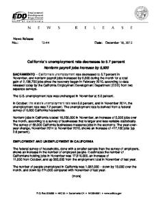
should also be noted that our simplifying assumption used here of a linear training cost function implies that the economy’s natural rate jumps immediately from the old level to the new steady-state level in response to a change in one or more of the theory’s parameters. If we assume instead that the training cost function is convex as in Hoon and Phelps (1992), so that instead of T (h) = βh as assumed here, we have T (0) = 0; T 0 (h) > 0; T 00 (h) > 0, the theory implies a gradual adjustment of the natural rate in response to an economic shock. Thus the theory when supplemented by a convex training cost implies persistence. 3. Empirical Tests on Singapore Data The big swings in Singapore’s unemployment rate occurred in the context of generally low and stable inflation rates. See Figure 1. In this section, we will first investigate the powers of the key variables identified in our theoretical model in explaining the movements of the natural rate of unemployment empirically. Next, we will explain how the natural rate of unemployment is estimated from a structural vector autoregression model (VAR), examine the impulse response functions, variance decompositions, and Granger causality tests. We need an estimate of the distance to frontier for Singapore. We take the US to be the frontier economy in our empirical exercise. Following the setup in Jones (2002), we compute the multifactor productivity for US, AU S , which is an efficiency level augmentation to the labor employed in the aggregate production function. The multifactor productivity for Singapore, AS , is computed likewise, with details given in Ho and Hoon (2006). We define the distance to frontier, Dist as the

AU S AS

− 1. A decrease in this measure implies that Singapore is closing

in to the world’s technology frontier. Our theoretical model predicts that an increase in the ratio of the wage paid at the individual firm to the expected wage paid elsewhere in the economy will reduce the natural rate as workers value their current job more and quit less. For empirical purposes, the ratio of wage received relative to expected wage paid elsewhere is proxied by ln At − (ln Et At ). If, following Blanchard (2000), the expected growth rate of technology is written as a weighted average of last period’s expectation of and current period’s actual growth rate, Et g(At ) = λEt−1 g(At−1 ) + (1 − λ)g(At ) with the weight, λ, being given by the ratio of the variance of the transitory component of technology growth to the sum of the variances of permanent 9

and transitory components of technology growth, it can be shown that ln At − (ln Et At ) = λg(At ) − λT Et−T g(At−T ) − (1 − λ)

PT −1 i i=1 λ g(At−i ). As T tends to infinity, we would have P∞ i

ln At − (ln Et At ) = λg(At ) − (1 − λ)

i=1

λ g(At−i ) given λ < 1. If the variance of the per-

manent component is much smaller than that of the transitory component, then λ is close to unity and ln At − (ln Et At ) would be close to g(At ) plus infinite lags of g(At ) with very small coefficients. Our estimates show that the ratio of the variance of transitory shocks to the sum of variances of permanent shocks and transitory shocks is 0.997, that is, λ = 0.997, suggesting that lags of g(At ) will be statistically insignificant in the regressions. Table 1 shows the regressions on the determinants of the natural rate. Specifications (1) and (3) are preferred to (2) and (4) because Durbin’s alternative test for autocorrelation shows that including the lagged dependent variable on the right-hand side is appropriate. This provides empirical support for including a convex training cost function in the theoretical model, which implies persistence in the natural rate. Looking at specification (1), 50 percent of last period’s natural rate persists into the current period. The effectiveness of assessing frontier technology via the ratio of imports of machinery from the G5 and the ratio of tertiary enrolment to employment, and the distance to frontier together represent g(A), which is specified in eq. (1) of our theoretical model. A positive shock to the distance to frontier (D.Dist) will reduce the natural rate significantly, consistent with our theoretical prediction. A one percent increase in the ratio of imports of machinery from the G5 (lnG5MT Y) will reduce the natural rate by 0.023 percentage points. An increase in the quality of learning, proxied by the ratio of tertiary enrolment to employment (lnIHL Emp), either current or lagged by one period, does not have a statistically significant impact on the natural rate. In the sample period, technology transfer via imports appears to be a more important channel of reducing the natural rate than the learning channel. To proxy for v/v e , which has a negative impact on the natural rate as stated in the Proposition, we will use the growth rate of technology and its lags, which can be computed. Empirically, a one percentage point increase in the growth rate of technology will reduce the natural rate by 0.12 percentage points. Note that the coefficient of the lag of the growth rate of technology is statistically not different from zero. In separate regressions not reported here, we have added lags of the growth rate of technology up to five years on the right-hand side and all the lags are statistically insignificant. Since these lags 10

are statistically insignificant, we may infer that a one percent increase in the productivity level relative to the perceived level of productivity (our proxy for the wage received relative to expected wage paid elsewhere) will reduce the natural rate by 0.12 percentage points. Changes in capital per employed worker have no statistically significant impact on the natural rate, consistent with the theoretical prediction although the variable in the model is capital per unit of labor force. (We have tried capital stock divided by population and it remains insignificant.) Similarly, marginal product of capital (MPK), used here as a proxy for the external real rate of interest, has no statistically significant impact on the natural rate, which is, unfortunately, not a prediction of our theoretical model; nevertheless, the coefficient has the correct sign. We find similar results in specification (3), which uses a lag of the log of tertiary enrolment to employment ratio in case its current value is endogenous. A structural vector autoregression (VAR) model of capital per worker, inflation, unemployment rate, and technology is used to estimate the time-varying steady state of the unemployment rate, defined as the natural rate.7 In the structural VAR model, the natural rate is driven by structural shocks which have permanent effects on the unemployment rate. We do not impose any smoothness restrictions arbitrarily on the natural rate. Guided by our theoretical model, we do allow technology shocks to have a permanent effect on the unemployment rate, apart from the impact of the natural rate shock. t t Consider the vector xt = [ln K , ln Pt , U nemt , ln At ], where ln K is the natural log of real Nt Nt

capital per worker, ln Pt is the natural log of the consumer price index, U nemt is the average unemployment rate in year t, and ln At is the natural log of technology level or multifactor productivity. Assume the first-differences of these four endogenous variables form a stationary VAR model: ∆xt = c +

J X

Fj ∆xt−j + et

(8)

j=1

where c is a vector of constants, Fj is a matrix of coefficients, and et is a vector of forecast errors normally distributed with zero mean. For our sample from 1966 to 2003, the pre-estimation lag-order selection statistics such as the final prediction error (FPE) and the Hannan and Quinn information criterion (HQIC) suggest a lag order J of 2 years. The post-estimation 7

King and Morley (2007) derive the natural rate for the US economy based upon a structural VAR with

real GDP, inflation and the unemployment rate.

11

Akaike’s information criterion (AIC) together with FPE and HQIC suggest a lag order of 2 years. The VAR model explains 32 percent, 75 percent, 25 percent, and 11 percent of the annual variation in capital per worker growth, inflation, change in unemployment, and growth in technology, respectively. Next we impose restrictions on the long-run relationship between the observables and the structural shocks. An infinite-order moving-average process represents the structural model: ∆xt = m +

∞ X

Cj vt−j

(9)

j=0

where m represents a vector of deterministic drifts for the variables in xt , Cj represents a matrix of shock coefficients, and vt represents a vector of four structural shocks with zero means, unit variances, and zero cross correlations. We assume that the shock coefficients satisfy the conditions for stationarity and impose the following long-run identifying restrictions: ∞ X j=0

c12,j = 0,

∞ X j=0

c31,j = 0,

∞ X j=0

c32,j = 0,

∞ X j=0

c41,j = 0,

∞ X j=0

c42,j = 0,

∞ X

c43,j = 0

(10)

j=0

where crc,j is the (r, c)-th element of Cj . Growth in capital per worker is not influenced in the long run by the second structural shock, which is named the AD or price shock. In the long run, changes in the unemployment rates are not affected by the first and second structural shocks, namely the capital intensity (KI) shock and the AD shock. The fourth structural shock, called the technology shock is the only structural shock having a long-run impact on the growth of technology. The third structural shock, or the natural rate (NRU) shock, together with the technology shock, will have a long-run impact on the changes in unemployment rate. This specification is consistent with our theoretical model where technology shocks play a role in determining the natural rate of unemployment. Figures 2A to 2D depict the structural impulse response functions given one standard deviation of the capital intensity (KI) shock, the AD or price shock, the natural rate (NRU) shock, and the technology shock, respectively. Despite a short-run negative impact on unemployment and a positive impact on technology, the KI shock has no lasting impact on unemployment and technology. However, it has a permanent impact on both capital per worker and inflation. The AD or price shock has no long-run impact on capital per worker, unemployment rate, and technology but has a persistent effect on inflation. Interestingly, its short-run impact on unemployment rates exhibits fluctuations which die off in the long run. The NRU shock does 12

not have a persistent effect on capital per worker and technology. It seems to have a very small and negative long-run impact on inflation. Its primary lasting influence is on the unemployment rate. The technology shock has a large and negative long-run impact on unemployment, and positive permanent effects on capital per worker and technology. Its influence on inflation is transitory and relatively small. Hence, Figure 2D provides a pictorial support for why we have included variables related to and explaining technology shocks in the regressions above. Table 2 presents the forecast error variance decompositions of innovations of capital per worker, inflation, unemployment rate, and technology. In the long run (looking at the variance decomposition at 20 years out), KI shocks explain the bulk of the variance of capital per worker (66.9 percent), followed by technology shocks (17.0 percent), and NRU shocks (11.2 percent). AD or price shocks have a minor role, consistent with the long-run restrictions imposed on the structural VAR model. The variance of inflation can be decomposed into KI shocks (16.0 percent), AD or price shocks (37.6 percent), NRU shocks (42.7 percent), and technology shocks (3.7 percent). Changes in the unemployment rate are mainly explained by NRU shocks (74.1 percent) and technology shocks (17.7 percent). KI shocks and AD or price shocks play minor roles, consistent with long-run identifying restrictions. The bulk of the movements in technology is explained by technology shocks (77.2 percent). NRU shocks and AD or price shocks play minor roles, consistent with the long-run restrictions. However, KI shocks explain 17.0 percent of the variance, which is not consistent with the long-run restrictions. As our focus in on the natural rate, this surprising last result will not affect our findings on the natural rate. We also perform Granger causality Wald tests on the underlying VAR model. Table 3 shows that innovations in capital per worker, unemployment, and technology separately and jointly Granger cause inflation. More importantly, innovations in technology Granger cause changes in unemployment, again highlighting the role of technology shocks in explaining unemployment, consistent with our theoretical model. The results in Table 3 for the underlying VAR model are consistent with the long-run identifying restrictions imposed on the structural model. After estimating the model, we check that all the eigenvalues lie inside the unit circle; hence the estimated model satisfies the eigenvalue stability condition. We also perform a 13

Lagrange-multiplier (LM) test for autocorrelation in the residuals of the estimated model. The test results suggest that there is no autocorrelation in the residuals for various lag orders from 1 to 10. To test whether the disturbances are normally distributed, we perform the Jarque-Bera test, the Skewness test, and the Kurtosis test. Considering all the equations together, all these tests show that the null hypothesis of normality cannot be rejected at 10 percent level of statistical significance. Based on the structural VAR model, innovations in the natural rate are driven by the implied long-run effects of the NRU shock and the technology shock. A sum of these innovations over time, together with the deterministic drift estimated from the underlying VAR model, will hence determine the level of the natural rate after we assume an initial level of natural level. The initial level is chosen such that the deviation of the actual unemployment rate from the natural rate, or cyclical unemployment, is zero on average over the entire sample. Figure 3 depicts our derived natural rate and the actual employment rate. We see that the natural rate comoves with the actual unemployment rate over the years. The standard deviation of innovations in our derived natural rate is 0.6845 while the innovations in the implied cyclical unemployment rate have a standard deviation of 0.5153. Hence, permanent shocks and transitory shocks to the actual unemployment rates are of comparable magnitude. 4. Role for Monetary Policy The basic picture that emerges from our study of the forces shaping the long swings of the unemployment rate in Singapore, bringing it down from nearly nine percent in 1966 to the lows of 2 to 3 percent in the 1990s, is one of technological catch up lowering the natural rate of unemployment. It is not expansionary monetary policy that has brought down the unemployment rate. Instead, the rapid productivity growth that accompanied the country’s openness to the international flow of ideas lifted the demand wage curve and lowered the supply wage curve. First, the rapid technological catch up stimulated hiring as the present discounted value of the future contributions of a trained employee increased. Moreover, the faster technical progress caused the real wage to run ahead of private wealth and acted to discourage labor turnover thus lowering the natural rate. In addition, it can be argued that, particularly in the early years of rapid growth, workers’ perception of the productivity level 14

in the rest of the economy fell behind the actual productivity each experienced in his or her individual firm so the wage expected elsewhere in the economy relative to the wage received by the worker (v e /v) was generally low. This further helped to stem rampant quitting and lowered the natural rate. Monetary policy was aimed, especially since 1981, to anchor inflation expectations in the region of two to three percent annually. To anchor the public’s inflation expectations, many Central Banks today adopt a form of inflation targeting, whether explicit or implicit. (Singapore practises implicit inflation forecast targeting using the exchange rate as an instrument, as opposed to an interest rate rule adopted in many other countries.) They aim toward transparency and effective communication with the public regarding future scenarios with the view of achieving an implicit or explicit inflation target. By anchoring the inflation expectations, the economy’s deviation from the natural rate is minimized. Yet nothing ensures that the natural rate of unemployment itself will not be inoptimally high. One conclusion that several economists studying the steady rise of European unemployment since the early 70s have drawn is that the slowdown in TFP growth since around 1973 was not well understood so that the perceived productivity level exceeded the actual productivity level with the consequence that the wage expected elsewhere was perceived to be higher than the wage paid at individual firms. See Phelps (2002), Nickell, et al. (2005) and Blanchard (2006). This led to an increase in the supply wage exceeding the demand wage with the result that the natural rate was increased. It appears that an important function of the Central Bank is to study explicit models of the determination of the natural rate of unemployment with as long a data series as is feasible. From the perspective of our model, getting to understand the determination of the path of equilibrium unemployment requires a deeper understanding of the forces that drive medium to long run growth. Figures 4a and 4b and Table 4 illustrate the Okun’s Law relationship for Singapore. The value of the constant term in Table 4 gives the minimum growth rate of real GDP required in order for the current unemployment rate to remain unchanged. (Any lower real GDP growth rate below this minimum implies rising unemployment.) The value of the constant went down from 9.1 percent for the period 1967-1984 to 6.3 percent for the period 1984-2003. It appears that the working public has adjusted its growth forecast from the 1967-84 period to the latter period. Yet, based on estimates of the latter period, the Singapore economy will have to 15

generate a real GDP growth rate of 6.3 percent annually if it is to keep the unemployment rate from steadily rising. It is an important task of the Central Bank, working in co-operation with other government agencies, to conduct research on growth models that can give realistic forecasts of medium to long term growth since this will have an impact on wage aspirations and consequently affect the natural rate. If movements of the unemployment rate mainly reflect fluctuations in the natural rate, is there any stabilization role for monetary policy in the short run? Does there exist a stable short-run Phillips curve when inflation expectations are well anchored in an economy with a time-varying natural rate? Tables 5 and 6 and Figure 5a show that in our whole sample period, there is no stable Phillips curve in the sense of a statistically significant negative relationship between the inflation rate and cyclical unemployment (calculated as the gap between the actual unemployment rate and the time-varying natural rate). This may reflect the fact that inflation expectations were shifting at various times, particularly the years surrounding the two oil price shocks. We find that when we restrict the sample to points where the inflation rate is equal to or below two percent (see Figure 5b), there does exist a statistically significant negative relationship between the inflation rate and cyclical unemployment.8 It appears, therefore, that despite the big movements in the natural rate, in the present low-inflation environment there is some scope for the Central Bank to engage in monetary policy to affect the output gap. Parrado (2004) argues that a monetary rule that makes the nominal trade-weighted exchange rate a function of the gap between the forecast and target inflation as well as the output gap (similar in form to the familiar Taylor Rule with the exception that the nominal exchange rate rather than the interest rate is used as an instrument) describes Singapore’s monetary policy very well. Implementation of the monetary rule requires an estimate of the natural 8

Akerlof et al. (1996) have argued that below two percent rate of inflation, there exists a negative rela-

tionship between the inflation rate and the actual unemployment rate. Table 5 does indeed show that in our restricted sample for points with inflation rate below two percent, a statistically significant relationship exists between the inflation rate and actual unemployment rate (coefficient of -0.240) at the ten percent level of significance. The Akerlof et al. model does not contain a natural rate defined as the unemployment rate that is inflation-invariant. Our theory, however, contains a natural rate, which allows us to calculate a measure of cyclical unemployment. We find a statistically significant relationship between the inflation rate and cyclical unemployment (coefficient of -0.519) at the 5 percent level of significance.

16

rate of unemployment. Our comment in the last paragraph about the need to study models of the determination of the natural rate of unemployment using long data series applies here to our discussion of stabilization policy since a wrong estimate of the natural rate can lead to overly deflationary policy if the natural rate is overestimated and overly inflationary policy if the natural rate is underestimated.9 5. The Case of Ireland It is interesting to observe that Ireland experienced big swings in unemployment rates from 1968 to 2005 as shown in Figure 6. Like Singapore, Ireland has also caught up with the technology frontier over the past few decades. Hence, in this section, we will re-do the key empirical exercises done in section 3 now using data on Ireland. Table 7 shows the regressions on the determinants of the natural rate in Ireland. As in the case of Singapore, the lag of the natural rate is highly significant, implying persistence in the natural rate. Under specification (1), 47.7 percent of last period’s natural rate persists into the current period for the case of Ireland. It is about 50 percent for Singapore. The effectiveness of assessing frontier technology via imports of G5 machinery and quality of learning has a significant impact on the natural rate in Ireland. A one percent increase in the ratio of imports of G5 machinery to GDP will decrease the natural rate by 0.091 percentage points while a one percent increase in the quality of learning, proxied by the average years of schooling, will reduce the natural rate by 0.2 percentage points. We have used average years of schooling for Ireland to obtain a longer time series for our regression analysis. If the ratio of tertiary enrollment to employment is used instead, the sample size will be reduced to less than 17 years. A longer time series is preferred so that it is more comparable with the case of Singapore. Both machine imports and learning are significant channels of technology transfer for the case of Ireland. Distance to frontier, however, has no significant impact on the natural rate in Ireland. To examine how the wage received relative to wages paid elsewhere may affect the natural rate, we look at the coefficients of D.lnA and its lags. We do not find any significant effect in specifications (2) and (4) with 3 lags. Adding more lags does not change the results. A one percent increase in the capital per employed worker will increase the natural rate of unemployment by more 9

This message has an echo in the Orphanides (2003a, 2003b) analysis of US inflation in the 1970s.

17

than 0.15 percentage points. This result is not predicted by the model but suggests a wealth effect which may increase the natural rate of unemployment. Long term interest rates have no significant impact on the natural rate, different from the theoretical prediction. Table 8 shows the forecast error variance decomposition for the structural VAR model of Ireland. At 20 years, NRU shocks and technology shocks explain 29.6 percent and 44.3 percent, respectively, of changes in capital per worker. The bulk of the variance in inflation is explained by KI shocks (23.7 percent) and AD or price shocks (55.3 percent). Technology shocks contribute 15.9 percent. Changes in the unemployment rate are explained by the AD or price shocks (53.4 percent) and technology shocks (25.5 percent). Movements in technology are mainly explained by technology shocks (40.4 percent) and NRU shocks (30.2 percent), followed by AD or price shocks (26.8 percent). The influence of AD or price shocks on unemployment rates and technology in the long run reflects the fact that in the whole sample period, Ireland did not have price or inflation stability. Based on the structural VAR model, we derive the natural rate of unemployment in Ireland and depict it in Figure 7, together with the actual unemployment rate. Similar to the case of Singapore, we run Phillips curve regressions on Ireland and the results are reported in Table 9. The impact of cyclical unemployment on inflation is statistically insignificant, implying that a stable short-run Phillips curve does not exist in Ireland over the whole sample period. We cannot run a regression for years with low inflation (less than or equal to 2 percent) as the sample will be reduced to only four years. As shown in Figure 8, inflation rates are high and vary widely without a stable relationship with cyclical unemployment. In contrast, the case of Singapore shows a regime of stable prices with a stable short-run Phillips curve at low inflation rates, as depicted in Figures 5A and 5B. 6. Conclusion Our study of the forces shaping the long swings of the unemployment rate in Singapore, bringing it down from nearly nine percent in 1966 to the lows of 2 to 3 percent in the 1990s, is one of technological catch up lowering the natural rate of unemployment. It is not expansionary monetary policy that has brought down the Singapore unemployment rate. Instead, the rapid productivity growth that accompanied the country’s openness to the international 18

flow of ideas lifted the demand wage curve and lowered the supply wage curve thus lowering structural unemployment. AD or price shocks play a bigger role in Ireland. In both Singapore and Ireland, the effectiveness of assessing frontier technology via imports of G5 machinery has a significant negative impact on the natural rate of unemployment. The Nelson-Phelps channel of learning has also played a significant role in lowering Ireland’s natural rate of unemployment. Our analysis suggests that an important task of the Central Bank is to conduct research on growth models that can give realistic forecasts of medium to long term growth since this will have a big impact on structural unemployment. References Akerlof, George, William Dickens and George Perry, 1996, “The Macroeconomics of Low Inflation,” Brookings Papers on Economic Activity, Vol. 1, pp. 1-76. Bianchi, Marco and Gylfi Zoega, 1998, “Unemployment Persistence: Does the Size of the Shock Matter?” Journal of Applied Econometrics, Vol. 13, No. 3 (May - Jun.), pp. 283-304. Blanchard, Olivier, 1985, “Debts, Deficits, and Finite Horizons,” Journal of Political Economy, Vol. 93 (Apr.), pp.223-247. Blanchard, Olivier, 2000, “Lecture 1: Shocks, Factor Prices , and Unemployment,” Lionel Robbins Lectures, London School of Economics. Blanchard, Olivier J., 2006, “European Unemployment: The Evolution of Facts and Ideas,” Economic Policy (Jan.), pp. 5-59. Blanchard, Olivier J. and Lawrence H. Summers, 1986, “Hysteresis and the European Unemployment Problem,” in Stanley Fischer (ed.), NBER Macroeconomics Annual, Vol. 1 (MIT Press, Cambridge, MA), pp. 15-78. Calmfors, Lars and Bertil Holmlund, 2000, “Unemployment and Economic Growth: A Partial Survey,” Swedish Economic Policy Review, Vol. 7, pp. 107-153. Coe, David T., Elhanan Helpman and Alexander W. Hoffmaister 1997, “North-South R&D Spillovers,” Economic Journal, Vol. 107, No. 440, pp. 134-149. Friedman, Milton, 1968, “The Role of Monetary Policy,” American Economic Review, Vol. 58, No. 1 (Mar.), pp. 1-17. Ho, Kong Weng and Hian Teck Hoon, 2006, “Growth Accounting for a Follower-Economy in 19

a World of Ideas: The Example of Singapore,” SMU Economics and Statistics Working Paper Series, Paper No. 15-2006, Singapore Management University. Hoon, Hian Teck and Edmund S. Phelps, 1992, “Macroeconomic Shocks in a Dynamized Model of the Natural Rate of Unemployment,” American Economic Review, Vol. 82 (Sep.), pp. 889-900. Hoon, Hian Teck and Edmund S. Phelps, 1997, “Growth, Wealth and the Natural Rate: Is Europe’s Jobs Crisis a Growth Crisis?” European Economic Review (Papers and Proceedings), Vol. 4, pp. 549-557. Jones, Charles I., 2002, “Sources of U.S. Economic Growth in a World of Ideas,” American Economic Review, Vol. 92, No. 1, pp. 220-239. King, Thomas B. and James Morley, 2007, “In Search of the Natural Rate of Unemployment,” Journal of Monetary Economics, Vol. 54, pp. 550-564. Layard, Richard, Stephen Nickell and Richard Jackman, 1991, Unemployment: Macroeconomic Performance and the Labour Market (Oxford University Press, Oxford). Nelson, Richard R. and Edmund S. Phelps, 1966, “Investment in Humans, Technological Diffusion, and Economic Growth,” American Economic Review (Papers and Proceedings), Vol. 56, pp. 69-75. Nickell, Stephen, Luca Nunziata and Wolfgang Ochel, 2005, “Unemployment in the OECD Since the 1960s. What Do We Know?” Economic Journal, Vol. 115 (Jan.), pp. 1-27. Papell, David H., Christian J. Murray and Hala Ghiblawi, 2000, “The Structure of Unemployment,” Review of Economics and Statistics, Vol. 82, No. 2 (May), pp. 309-315. Parrado, Eric, 2004, Singapore’s Unique Monetary Policy: How Does It Work?, Monetary Authority of Singapore Staff Paper No. 31, (Jun) (Monetary Authority of Singapore, Singapore). Phelps, Edmund S., 1968, “Money-Wage Dynamics and Labor Market Equilibrium,” Journal of Political Economy, Vol. 76 (July/August, Part 2), pp. 678-711. Phelps, Edmund S., 1994, Structural Slumps: The Modern-Equilibrium Theory of Unemployment, Interest and Assets (Harvard University Press, Cambridge, MA). Phelps, Edmund S., 2002, “Unemployment in Europe: Reasons and Remedies,” Keynote Address to the Conference on Unemployment in Europe, CESifo Conference Centre, Munich, 20

6-7 December 2002. Pissarides, Christopher, 1990, Equilibrium Unemployment Theory (Basil Blackwell, Oxford). Salop, Steven C., 1979, “A Model of the Natural Rate of Unemployment,” American Economic Review, Vol. 69 (Mar.), pp. 117-125.

21

Table 1: Determinants of the Natural Rate of Unemployment in Singapore Coefficients (t-statistics based on robust std. err.) NatRate (1) (2) (3) (4) L.NatRate 0.5032 0.5152 (3.92)*** (3.61)*** D.Dist -13.3172 -14.2394 -13.4695 -14.2374 (-2.17)** (-2.16)** (-2.13)** (-2.05)* lnG5MT_Y -2.2790 -2.8570 -2.5405 -3.0870 (-2.34)** (-2.61)** (-3.01)*** (-3.69)*** lnIHL_Emp 0.6057 1.7238 (0.35) (0.75) L.lnIHL_Emp -0.1200 1.2372 (-0.08) (0.71) D.lnA -12.4159 -13.6487 -12.5904 -13.2286 (-2.74)** (-2.49)** (-2.68)** (-2.30)** L.D.lnA 1.2035 0.1699 1.2591 -0.0919 (0.59) (0.06) (0.62) (-0.03) lnK_N 0.9174 -0.0116 1.8134 0.6139 (0.43) (-0.00) (1.04) (0.28) MPK 3.8861 13.5559 10.7483 16.5786 (0.19) (0.47) (0.54) (0.60) Constant -10.1601 4.5157 -24.3566 -5.1054 (-0.30) (0.10) (-0.86) (-0.15) 2 R 0.8219 0.7345 0.8211 0.7343 Durbin-Watson 2.0861 1.0698 2.1418 1.1128 Observations 33 34 33 34 Notes: The t-statistics is computed based on robust standard error. L and D denote the lag operator and the first difference operator respectively. * ** , , and *** denote 10%, 5%, and 1% statistical significance respectively. Durbin’s alternative test for autocorrelation shows that there is no serial correlation up to 4 lags under specification (1) and up to 3 lags under specification (3). When lnK_N is replaced by the logarithm of real capital stock per capita, instead of per employed worker, the qualitative results remain unchanged. The results remain the same qualitatively when lags of D.lnA are included up to the 5th year. The coefficients of all lags of D.lnA are statistically insignificant. D.lnA and its lags together represent v/ve, which has a negative impact as stated in the Proposition. The impact of g(A), specified in equation (1) of our theoretical model, on the natural rate works through the effectiveness of assessing frontier technology proxied by lnG5MT_Y and lnIHL_Emp, and through shocks to the distance to frontier D.Dist.

Table 2: Forecast Error Variance Decomposition: Singapore Capital Per Worker Year KI AD NRU Shock Shock Shock 1 77.6% 3.1% 6.7% 5 67.7% 4.7% 10.5% 20 66.9% 4.9% 11.2%

Tech. Shock 12.6% 17.1% 17.0%

Inflation KI AD Shock Shock 22.5% 70.6% 16.3% 39.2% 16.0% 37.6%

Unemployment Rate NRU Tech. KI AD NRU Shock Shock Shock Shock Shock 6.6% 0.3% 3.1% 0.6% 96.3% 41.1% 3.5% 3.5% 4.6% 74.1% 42.7% 3.7% 3.5% 4.7% 74.1%

Technology Tech. KI AD Shock Shock Shock 0.0% 14.7% 0.1% 17.8% 17.0% 1.2% 17.7% 17.0% 1.3%

NRU Shock 2.3% 4.0% 4.5%

Tech. Shock 82.9% 77.8% 77.2%

Notes: KI, AD, NRU, and Tech denote capital intensity shock, aggregate demand or price shock, natural rate shock, and technology shock respectively.

Table 3: Granger Causality Wald Test: Singapore Equation D.lnK_N D.lnK_N D.lnK_N D.lnK_N D.lnP D.lnP D.lnP D.lnP D.Unem D.Unem D.Unem D.Unem D.lnA D.lnA D.lnA D.lnA

Excluded D.lnP D.Unem D.lnA All D.lnK_N D.Unem D.lnA All D.lnK_N D.lnP D.lnA All D.lnK_N D.lnP D.Unem All

F 0.9638 0.1013 2.0659 1.4114 7.9622 14.355 8.3048 5.72 1.5944 0.26069 3.5807 1.3522 0.3180 0.7537 0.1549 0.4146

Prob. > F 0.3946 0.9040 0.1470 0.2479 0.0020*** 0.0001*** 0.0016*** 0.0007*** 0.2223 0.7725 0.0423** 0.2706 0.7304 0.4806 0.8573 0.8626

Notes: ** , and *** denote that the null hypothesis that there is not Granger causality is rejected at 5% and 1% statistical significance respectively. The results show that D.lnK_N, D.Unem, D.lnA separately and jointly Granger cause D.lnP. Also, D.lnA Granger causes D.Unem, consistent with our theoretic model. The test results are consistent with the long-run restrictions in our SVAR model.

Table 4: Minimum Growth in Total Real GDP to Maintain Constant Unemployment Rate in Singapore Growth in GDP Change in Unemployment Constant R2 Observations

1967-2003 (1) -2.0880*** 7.3433*** 0.2678 39

1967-1984 (2) -0.5092 9.1176*** 0.0337 18

1984-2003 (3) -3.0247*** 6.3135*** 0.4631 22

Notes: *** denotes 1% statistical significance. The 95% confidence intervals of the constant term in (2) and (3) do not overlap, suggesting that they are statistically different from one another.

Table 5: Regressing Inflation on Natural Rate, Unemployment, and Cyclical Unemployment in Singapore

Inflation Natural Rate Unemployment Cyclical Unemployment Constant R2 Observations

(1) -0.697

Inflation ≤ 2% (2) (3) -0.187 -0.161

Inflation ≤ 2% (4) (5) -0.240* 0.417

5.328** 1.313 0.0337 0.0436 36 19

3.368** 1.527*** 0.0052 0.1866 40 21

Inflation ≤ 2% (6) -0.519**

2.861*** 0.448** 0.0068 0.2965 36 19

Notes: * ** , , and *** denote 10%, 5% and 1% statistical significance respectively. There exists no statistical significant negative relation between inflation and the natural rate (no long-run Phillips curve); however, there is a statistical significant negative relation between inflation and cyclical unemployment for the sample with inflation less than or equal to 2 percent. Hence, it is important to distinguish the different relations.

Table 6: Phillips Curve Regression Results for Singapore Inflation ≤ 2% Inflation (1) (2) (3) Inflation (1-2 lags) 0.5272 0.4637 0.3486 (6.32)** (5.66)* (1.81) Cyclical Unemployment (0-1 lag) 0.4697 (0.87) Cyclical Unemployment (0-2 lags) 0.2927 -0.2968 (0.21) (4.87)* Capital Intensity Shocks (0-1 lag) 27.0653 (2.13) Capital Intensity Shocks (0-2 lags) -5.8901 1.9796 (0.08) (0.11) Technology Shocks (0-1lag) -3.1209 (0.04) Technology Shocks (0-2 lags) 75.0828 9.6234 (2.03) (1.49) R2 0.7182 0.9435 0.5926 Observations 34 17 35

Inflation ≤ 2% (4) 0.3490 (5.09)* -0.3445 (6.52)** 4.6160 (3.08) 2.6453 (0.44) 0.9092 18

Notes: χ2-statistics for the sum of coefficients computed using robust standard errors are reported in parentheses. * , and ** denote 10% and 5% statistical significance respectively. R2’s are computed with no constant in the regressions. Compared to Table 5, Table 6 presents a more sophisticated test of the existence of the Phillips curve. After considering dynamics and controlling for capital intensity shocks and technology shocks, the impact of cyclical unemployment on inflation is now smaller: a one percentage point increase in cyclical unemployment corresponds to a cumulative 0.2968 percentage point decrease in inflation after 2 years, as given in specification (2) where the sample is restricted to periods of low inflation. The shortrun Phillips curve exists only for low inflation; in fact, using the entire sample, there is no statistical significant negative relation between inflation and cyclical unemployment. With a different lag structure, specification (4) similarly demonstrates the existence of the short-run Phillips curve for the sample restricted to low inflation periods.

Table 7: Determinants of the Natural Rate of Unemployment in Ireland Coefficients (t-statistics based on robust std. err.) NatRate (1) (2) (3) (4) L.NatRate 0.477 0.503 0.501 0.533 (3.19)*** (3.16)*** (3.15)*** (3.41)*** D.Dist 9.434 6.269 18.414 17.982 (0.67) (0.43) (1.51) (1.47) -8.937 lnG5MT_Y -9.117 -9.794 -9.958 (-3.73)*** (-3.22)*** (-3.87)*** (-4.01)*** -20.671 lnSchool -20.090 ** (-2.14)** (-2.52) L.lnSchool -21.090 -21.667 (-1.51) (-1.65) D.lnA -7.808 -12.522 12.807 10.638 (-0.70) (-0.87) (1.73)* (1.30) L.D.lnA -1.759 -0.322 -0.755 3.486 (-0.21) (-0.03) (-0.09) (0.28) L2.D.lnA -4.524 2.380 (-0.46) (0.24) L3.D.lnA 8.237 12.126 (0.80) (1.15) lnK_N 15.454 15.744 15.873 16.525 (3.94)*** (4.04)*** (2.65)** (2.91)*** LongRate -0.163 -0.148 -0.082 -0.005 (-1.10) (-0.70) (-0.59) (-0.03) Constant -150.768 -153.087 -157.013 -165.503 (-4.32)*** (-4.55)*** (-3.46)*** (-3.69)*** R2 0.8885 0.8955 0.8749 0.8844 Durbin-Watson 2.2934 2.3281 2.2497 2.3815 Observations 31 31 31 31 Notes: The t-statistics is computed based on robust standard error. L and D denote the lag operator and the first difference operator respectively. * ** , , and *** denote 10%, 5%, and 1% statistical significance respectively. Instead of log of tertiary enrollment over employment (lnIHL_EMP) as in the case of Singapore, we have used lnSchool, log of average years of schooling, to obtain a longer time series for Ireland; using lnIHL_Emp for Ireland will give less than 17 years of data. Durbin’s alternative test for autocorrelation shows that there is no serial correlation up to at least 6 lags for all specifications.

Table 8: Forecast Error Variance Decomposition: Ireland Capital Per Worker Year KI AD NRU Shock Shock Shock 1 1.6% 26.5% 46.4% 5 3.8% 21.5% 28.2% 20 10.0% 16.2% 29.6%

Tech. Shock 25.5% 46.6% 44.3%

Inflation KI AD Shock Shock 73.1% 25.8% 26.7% 58.3% 23.7% 55.3%

NRU Shock 0.3% 1.7% 5.1%

Tech. Shock 0.8% 13.3% 15.9%

Unemployment Rate KI AD NRU Shock Shock Shock 14.7% 71.8% 3.3% 13.4% 57.0% 5.5% 13.6% 53.4% 7.5%

Tech. Shock 10.2% 24.1% 25.5%

Technology KI AD Shock Shock 0.6% 24.4% 2.5% 26.8% 2.6% 26.8%

NRU Shock 31.1% 30.0% 30.2%

Tech. Shock 44.0% 40.8% 40.4%

Notes: KI, AD, NRU, and Tech denote capital intensity shock, aggregate demand or price shock, natural rate shock, and technology shock respectively.

Table 9: Phillips Curve Regression Results for Ireland Inflation Inflation (1-2 lags)

(1) (2) 0.840 0.806 (40.83)*** (38.02)*** Cyclical Unemployment (0-1 lag) -0.285 (1.35) Cyclical Unemployment (0-2 lags) -0.292 (1.74) Capital Intensity Shocks (0-1 lag) 19.205 (0.89) Capital Intensity Shocks (0-2 lags) 11.967 (0.29) Technology Shocks (0-1lag) 18.330 (3.66)* Technology Shocks (0-2 lags) 24.842 (5.14)** R2 0.9392 0.9278 Observations 38 39 Notes: χ2-statistics for the sum of coefficients computed using robust standard errors are reported in parentheses. * ** , , and ** denote 10%, 5%, and 1% statistical significance respectively. R2’s are computed with no constant in the regressions.

Figure 1: Unemployment and Inflation in Singapore 25

20

Percent

15

10

5

0 1966

1968

1970

1972

1974

1976

1978

1980

1982

1984

1986

1988

1990

1992

1994

1996

1998

16

17

2000

2002

18

19

2004

-5 Year Unemployment Rate

Inflation Rate

Figure 2A: Impulse Response Functions given KI Shock 0.1

0.05

0

Percent

0

1

2

3

4

5

6

7

8

9

10

11

12

13

14

15

-0.05

-0.1

-0.15

-0.2 Years after one standard deviation shock

Capital Per Worker

Inflation

Unemployment

Technology

20

Figure 2B: Impulse Response Functions given AD Shock 0.1

0.08

0.06

0.04

Percent

0.02

0 0

1

2

3

4

5

6

7

8

9

10

11

12

13

14

15

16

17

18

19

20

18

19

20

-0.02

-0.04

-0.06

-0.08

-0.1

-0.12 Years after one standard deviation shock

Capital Per Worker

Inflation

Unemployment

Technology

Figure 2C: Impulse Response Functions given NRU Shock 1.2

1

0.8

Percent

0.6

0.4

0.2

0 0

1

2

3

4

5

6

7

8

9

10

11

12

13

14

15

16

17

-0.2 Years after one standard deviation shock

Capital Per Worker

Inflation

Unemployment

Technology

Figure 2D: Impulse Response Functions given Technology Shock 0.1

0 0

1

2

3

4

5

6

7

8

9

10

11

12

13

14

15

16

17

18

19

Percent

-0.1

-0.2

-0.3

-0.4

-0.5 Years after one standard deviation shock

Capital Per Worker

Inflation

Unemployment

Technology

Figure 3: Natural Rate of Unemployment in Singapore, 1968 to 2003 9

8

7

Percent

6

5

4

3

2

1

0 1968

1970

1972

1974

1976

1978

1980

1982

1984

1986

1988

1990

1992

Year Natural Rate

Uemployment Rate

1994

1996

1998

2000

2002

Figure 4A: Growth Rate of Total Real GDP and Change in Unemployment in Singapore, 1967 to 1984 14

12

Growth Rate (Percent)

10

8

6

4

2

0 -4

-3

-2

-1

0

1

2

Change in Unemployment (Percent)

Figure 4B: Growth Rate of Total Real GDP and Change in Unemployment in Singapore, 1984 to 2003 14

12

10

Growth Rate (Percent)

8

6

4

2

0 -2

-1.5

-1

-0.5

0

0.5

1

-2

-4 Change in Unemployment (Percent)

1.5

2

2.5

3

Figure 5A: Inflation and Cyclical Unemployment in Singapore, 1968 to 2003 25

20

Inflation (Percent)

15

10

5

0 -2

-1.5

-1

-0.5

0

0.5

1

1.5

2

-5 Cyclical Unemployment (Percent)

Figure 5B: Low Inflation and Cyclical Unemployment in Singapore 2.5

2

1.5

Inflation (Percent)

1

0.5

0 -2

-1.5

-1

-0.5

0

0.5

-0.5

-1

-1.5

-2

-2.5 Cyclical Unemployment (Percent)

1

1.5

2

Natural Rate

Year

Unemployment Rate

20 00

19 98

19 96

19 94

19 92

19 90

Percent

Unemployment Rate

19 88

19 86

19 84

19 82

19 80

19 78

19 76

19 74

19 72

19 70

19 68

19 66

19 64

19 62

19 68 19 69 19 70 19 71 19 72 19 73 19 74 19 75 19 76 19 77 19 78 19 79 19 80 19 81 19 82 19 83 19 84 19 85 19 86 19 87 19 88 19 89 19 90 19 91 19 92 19 93 19 94 19 95 19 96 19 97 19 98 19 99 20 00 20 01 20 02 20 03 20 04 20 05

Percent

Figure 6: Unemployment and Inflation in Ireland

20

18

16

14

12

10

8

6

4

2

0

Year

Inflation Rate

Figure 7: Natural Rate of Unemployment in Ireland, 1962 to 2001

20

18

16

14

12

10

8

6

4

2

0

Figure 8: Inflation and Cyclical Unemployment in Ireland, 1968 to 2001 20

18

16

14

Inflation (Percent)

12

10

8

6

4

2

0 -5

-4

-3

-2

-1

0

1

Cyclical Unemployment (Percent)

2

3

4

5