Certainty Equivalence in Nonlinear Output Regulation with Unmeasurable Regulated Error Fabio Celani Department of Computer and Systems Science Antonio Ruberti Sapienza University of Rome, Italy
17th IFAC World Congress Seoul, South Korea July 10th , 2008
1 / 11
Nonlinear Output Regulation with Unmeasurable Regulated Error exosystem
w (0) ∈ W ⊂ Rd W compact and invariant
w˙ = s(w) w χ˙ = ϕ(χ, e) u = ρ(χ, e) measurement feedback regulator
u
x˙ = f (x, u, w) e = h(x, w) y = k(x, w)
e y
plant
x(0) ∈ X ⊂ Rn compact
u, e, y ∈ R
semiglobal output regulation find measurement feedback regulator and set ∆ of initial states such that 1. trajectories are bounded 2. limt→∞ e(t) = 0 uniformly w.r.t. initial state i.e. ∀� > 0 ∃T > 0 s.t. |e(t)| < � ∀t ≥ T ∀(x(0), w (0), χ(0)) ∈ X × W × ∆ full information regulation + uniform observability ⇒ certainty equivalence design
2 / 11
Outline
I
full information regulation
I
uniform observability
I
observer design
I
certainty equivalence design
3 / 11
Full Information Regulation exosystem
w (0) ∈ W ⊂ Rd W compact and invariant
w˙ = s(w) w full information regulator
u = u∗(x, w)
u
e
x˙ = f (x, u, w) e = h(x, w) y = k(x, w) x
y
plant
x(0) ∈ X ⊂ Rn compact u, e, y ∈ R
Assumption (full information regulation) there exists u ∗ (x, w ) s.t. x˙ w˙
= =
f (x, u ∗ (x, w ), w ) s(w )
satisfies the following 1. trajectories are bounded 2. limt→∞ e(t) = 0 uniformly w.r.t. initial state. if 1. holds, then 2. ⇔ (Byrnes-Isidori, 2003)
. A = ω(X × W ) ⊆ {(x, w ) : e = h(x, w ) = 0}
4 / 11
Uniform Observability exosystem
w (0) ∈ W ⊂ Rd W compact and invariant
w˙ = s(w) w u
x˙ = f (x, u, w) e = h(x, w) y = k(x, w) plant
e y
x(0) ∈ X ⊂ Rn compact u, e, y ∈ R
Assumption (uniform observability) there exists global diffeomorphism z = φ(x, w )
0
z˙ 1 z˙ 2 .. .
B B B z˙ = B B @ z˙ n ˜−1 z˙ n˜
1 C C C C C A y
z ∈ Rn˜
Gauthier-Kupka’s observability 0 F1 (z1 , z2 , u) B F2 (z1 , z2 , z3 , u) B B . = B .. B @ F n ˜−1 (z1 , z2 , . . . , zn ˜ , u) Fn˜ (z1 , z2 , . . . , zn˜ , u) =
n ˜ =d +n
canonical form 1 C C C C = F (z, u) C A
z(0) ∈ Z ⊂ Rn˜ compact
K (z1 )
∂Fi with (z1 , z2 , . . . , zi+1 , u) 6= 0 ∂zi+1 ∂K and (z1 ) 6= 0 ∂z1
i = 1, . . . , n ˜−1
5 / 11
Bound on z Trajectories coordinates plant + exosystem full information regulator closed-loop + exosystem compact attractor
(x, w ) x˙ w˙
= =
z = φ(x, w ) f (x, u, w ) s(w )
x(0) ∈ X w (0) ∈ W
= =
z(0) ∈ Z
. u ˜∗ (z) = u ∗ (φ−1 (z))
u ∗ (x, w ) x˙ w˙
z˙ = F (z, u)
f (x, u ∗ (x, w ), w ) s(w )
x(0) ∈ X z(0) ∈ Z
A
z˙ = F (z, u ˜∗ (z))
z(0) ∈ Z
A˜ ↓
converse Lyapunov (Marconi-Praly-Isidori)
proper Lyapunov functon V ˜ (z) ≤ b} ⊇ Z (Ωb compact) pick b > 0 s.t. Ωb = {z ∈ D|V z(0) ∈ Z ⇒ z(t) ∈ Ωb ∀t ≥ 0 if z˙ = F (z, u) is controlled by u = u ˜∗ (z) if z˙ = F (z, u) is controlled by the forthcoming measurement feedback regulator it will be shown that z(0) ∈ Z ⇒ z(t) ∈ Ωb+1 ∀t ≥ 0 6 / 11
Globally Lipschitz z-system plant+exosystem in Gauthier-Kupka’s observability canonical form z˙ y
= =
F (z, u) K (z1 )
(1)
it will be shown that system (1) controlled by the forthcoming measurement feedback regulator is such that I I
z(0) ∈ Z ⇒ z(t) ∈ Ωb+1 ∀t ≥ 0 (Ωb+1 compact) . u(t) ∈ U = [−l, l] where l = max |˜ u ∗ (z)| + 1 z∈Ωb+1
let F gl : Rn˜ × R → Rn˜ and K gl : R → R be such that I
F gl (z, u) = F (z, u) and K gl (z1 ) = K (z1 )
I
they satisfy Gauthier-Kupka’s global Lypschitz conditions
∀(z, u) ∈ Ωb+1 × U
globally Lipschitz z-system z˙ y
= =
F gl (z, u) K gl (z1 ) ,
(2)
z(t) ∈ Ωb+1 and u(t) ∈ U ⇒ (2) ≡ (1)
7 / 11
Observer for Globally Lipschitz z-system globally Lipschitz z-system z˙ y
= =
F gl (z, u) K gl (z1 ) ,
(3)
Gauthier-Kupka’s observer zˆ˙
=
F gl (ˆ z , u) + G (y − K gl (ˆ z1 ))
(4)
Thm. (Gauthier-Kupka) There exists G such that (4) is a global exponential observer of (3). ⇓ (4) is a global exponential observer of z˙ y
= =
F (z, u) K (z1 )
as long as z(t) ∈ Ωb+1 and u(t) ∈ U
8 / 11
Certainty Equivalence Design measurement feedback regulator zˆ˙ u
= =
F gl (ˆ z , u) + G (y − K gl (ˆ z1 )) satl (˜ u ∗ (ˆ z )) .
(5)
Proposition. (5) solves the semiglobal output regulation problem. Sketch of proof. Closed-loop system x˙ w˙ zˆ˙ e
= = = =
f (x, satl (˜ u ∗ (ˆ z )), w ) s(w ) F gl (ˆ z , satl (˜ u ∗ (ˆ z ))) + G (k(x, w ) − K gl (ˆ z1 )) h(x, w )
(6)
change of coordinates z = φ(x.w ) tranforms (6) into z˙ zˆ˙ e
= = =
F (z, satl (˜ u ∗ (ˆ z ))) F gl (ˆ z , satl (˜ u ∗ (ˆ z ))) + G (K (z1 ) − K gl (ˆ z1 )) H(z)
(7)
adapt arguments from (Teel-Praly, 1995), (Isidori, 1999), (Gauthier-Kupka, 2001), and (Marconi-Praly-Isidori, 2007) to prove that I trajectories are bounded and z(t) ∈ Ω b+1 ∀t ≥ 0 I z(t) − z ˆ(t) → 0 I e(t) → 0 uniformly w.r.t. initial state 9 / 11
Conclusions
I
nonlinear output regulation problem with unmeasurable regulated error solved by certainty equivalence design
I
lack of robustness with respect to either plant or exosystem uncertainties
10 / 11
Acknowledgments
I
Prof. A Isidori
I
Dr. C. De Persis
11 / 11