Derivative and Integral of the Heaviside Step Function Originally appeared at: http://behindtheguesses.blogspot.com/2009/06/derivative-and-integral-of-heaviside.html Eli Lansey —
[email protected] June 30, 2009
The Setup HHxL
HHxL
1.0
1.0
0.8
-4
-2
0.8
0.6
0.6
0.4
0.4
0.2
0.2
2
4
x
-100
-1. ´ 10
(a) Large horizontal scale
-101
-5. ´ 10
-101
5. ´ 10
x
-100
1. ´ 10
(b) “Zoomed in”
Figure 1: The Heaviside step function. Note how it doesn’t matter how close we get to x = 0 the function looks exactly the same. The Heaviside step function H(x), sometimes called the Heaviside theta function, appears in many places in physics, see [1] for a brief discussion. Simply put, it is a function whose value is zero for x < 0 and one for x > 0. Explicitly, ( 0 x < 0, H(x) = . (1) 1 x>0 We won’t worry about precisely what its value is at zero for now, since it won’t effect our discussion, see [2] for a lengthier discussion. Fig. 1 plots H(x). The key point is that crossing zero flips the function from 0 to 1. Derivative – The Dirac Delta Function Say we wanted to take the derivative of H. Recall that a derivative is the slope of the curve at at point. One way of formulating this is dH ∆H = lim . ∆x→0 ∆x dx
(2)
Now, for any points x < 0 or x > 0, graphically, the derivative is very clear: H is a flat line in those regions, and the slope of a flat line is zero. In terms of (2), H does not change, so ∆H = 0 and dH/dx = 0. But if we pick two points, equally spaced on opposite sides of x = 0, say x− = −a/2 1
∆ HxL
RHxL
a
- 21a
1 2a
x 0
(a) Dirac delta function
x
(b) Ramp function
Figure 2: The derivative (a), and integral (b) of the Heaviside step function. and x+ = a/2, then ∆H = 1 and ∆x = a. It doesn’t matter how small we make a, ∆H stays the same. Thus, the fraction in (2) is 1 dH = lim a→0 a dx = ∞.
(3)
Graphically, again, this is very clear: H jumps from 0 to 1 at zero, so it’s slope is essentially vertical, i.e. infinite. So basically, we have 0 x < 0 dH δ(x) ≡ = ∞ x=0. (4) dx 0 x>0 This function is, loosely speaking, a “Dirac Delta” function, usually written as δ(x), which has seemingly endless uses in physics. We’ll note a few properties of the delta function that we can derive from (4). First, integrating it from −∞ to any x− < 0: ¶ Z x− Z x− µ dH dx δ(x)dx = dx −∞ −∞ (5) = H(x− ) − H(−∞) =0 since H(x− ) = H(−∞) = 0. On the other hand, integrating the delta function to any point greater than x = 0: ¶ Z x+ Z x+ µ dH dx δ(x)dx = dx −∞ −∞ (6) = H(x+ ) − H(−∞) =1 since H(x+ ) = 1. At this point, I should point out that although the delta function blows up to infinity at x = 0, it still has a finite integral. An easy way of seeing how this is possible is shown in Fig. 2(a). If the 2
width of the box is 1/a and the height is a, the area of the box (i.e. its integral) is 1, no matter how large a is. By letting a go to infinity we have a box with infinite height, yet, when integrated, has finite area. Integral – The Ramp Function Now that we know about the derivative, it’s time to evaluate the integral. I have two methods of doing this. The most straightforward way, which I first saw from Prof. T.H. Boyer, is to integrate H piece by piece. The integral of a function is the area under the curve,1 and when x < 0 there is no area, so the integral from −∞ to any point less than zero is zero. On the right side, the integral to a point x is the area of a rectangle of height 1 and length x, see Fig. 1(a). So, we have ( Z x 0 x < 0, H dx = . (7) x x>0 −∞ We’ll call this function a “ramp function,” R(x). We can actually make use of the definition of H and simplify the notation: Z R(x) ≡ H dx = xH(x) (8) since 0 × x = 0 and 1 × x = x. See Fig. 2(b) for a graph – and the reason for calling this a “ramp” function. But I have another way of doing this which makes use of a trick that’s often used by physicists: We can always add zero for free, since anything + 0 = anything. Often we do this by adding and subtracting the same thing, A = (A + B) − B, (9) for example. But we can use the delta function (4) to add zero in the form 0 = x δ(x).
(10)
Since δ(x) is zero for x 6= 0, the x part doesn’t do anything in those regions and this expression is zero. And, although δ(x) = ∞ at x = 0, x = 0 at x = 0, so the expression is still zero. So we’ll add this on to H: H =H +0 = H + x δ(x) dH =H +x dx dH dx H +x = dx dx d = [xH(x)] , dx
by (4)
(11)
where the last step follows from the “product rule” for differentiation. At this point, to take the integral of a full differential is trivial, and we get (8). 1
To be completely precise, it’s the (signed) area between the curve and the line x = 0.
3
References [1] M. Springer. Sunday function [online]. February 2009. Available from: http://scienceblogs.com/builtonfacts/2009/02/sunday_function_22.php [cited 30 June 2009]. [2] E.W. Weisstein. Heaviside step function [online]. Available from: http://mathworld.wolfram.com/HeavisideStepFunction.html [cited 30 June 2009].
4