IMPACTS OF PRIMARY ENERGY CONSTRAINTS IN THE 21ST CENTURY
Willem P. Nel Student No. 909032873
Supervisor: Prof. H. J. Annegarn Co-supervisor: Prof. G. van Zyl
A thesis submitted in fulfilment of the requirements for the degree Doctor of Philosophy – Energy Studies in the Department of Geography, Environmental Management and Energy Studies University of Johannesburg, Johannesburg.
Revised after examination 12 April 2009
DECLARATION I declare that the thesis: “Impacts of primary energy constraints in the 21st Century” is my own work, that it has not been submitted for any degree or examination in any other university, and that all the sources I have used or quoted have been indicated and acknowledged by complete references. Three papers have been published or submitted for publication arising from this thesis: Nel, W.P., C.J. Cooper 2008: A Critical Review of IEA’s Oil Demand Forecast for China, Energy Policy, Vol. 36, No. 3, pp. 1096–1106. Nel, W.P., C.J. Cooper 2009: Implications of fossil fuel constraints on economic growth and global warming, Energy Policy, Vol. 37, No. 1, pp. 166-180. Nel, W.P., G. van Zyl 2008: Defining limits: Energy Constrained Economic Growth, Applied Energy, Submitted.
Willem P. Nel 17 November 2008
i
AFFIDAVIT TO WHOM IT MAY CONCERN
This serves to confirm that I, Willem P Nel, ID Number 6407195162087, Student number 909032873 enrolled for the qualification PhD (Energy Studies) thesis in the Faculty of Science, herewith declare that my academic work is in line with the Plagiarism Policy of the University of Johannesburg, with which I am familiar. I further declare that the work presented in the thesis Impacts of primary energy constraints in the 21st Century is authentic and original unless clearly indicated otherwise and in such instances full reference to the source is acknowledged and I do not pretend to receive any credit for such acknowledged quotations, and that there is no copyright infringement in my work. I declare that no unethical research practices were used or material gained through dishonesty. I understand that plagiarism is a serious offence and that should I contravene the Plagiarism Policy notwithstanding signing this affidavit, I may be found guilty of a serious criminal offence (perjury) that would amongst other consequences compel the UJ to inform all other tertiary institutions of the offence and to issue a corresponding certificate of reprehensible academic conduct to whomever request such a certificate from the institution. Signed at Johannesburg on this 17th day of November 2008
Signature Willem P. Nel
STAMP COMMISSIONER OF OATHS Affidavit certified by a Commissioner of Oaths This affidavit conforms with the requirements of the JUSTICES OF THE PEASE AND COMMISSIONERS OF OATHS ACT 16 OF 1963 and the applicable Regulations published in the GG GNR 1258 of 21 July 1972; GN 903 of 10 July 1998; GN 109 of 2 February 2001 as amended.
ii
ABSTRACT Global society has evolved into a complex multi-dimensional system in which it has become increasingly difficult to construct and maintain a systemic model of cause and effect. Specialisation and abstraction in the various disciplines of scientific and societal complexity has led to divergent theories of sustainability. Failure to integrate real life problems across disciplines poses a threat to modern society because the causal links between disciplines are unattended in many instances and events in one dimension could lead to catastrophic unintended consequences in another. In light of the above, this thesis contributes towards the multi-disciplinary integration of some of the most important sustainability concerns of modern society, namely Energy Security, Economic Growth and Global Warming. Analysing these real-life sustainability issues in a multi-disciplinary context leads to conclusions that are controversial in terms of established philosophical worldviews and policy trends. Firstly, the thesis establishes deterministic expectations of an imminent era of declining Energy Security resulting from the exhaustion of non-renewable fossil fuel resources, despite optimistic expectations of technology improvements in alternative energy sources such as renewable and nuclear. Secondly, the exhaustion of non-renewable fossil fuel resources imposes limits to the potential sources of anthropogenic carbon emissions that render the more pessimistic emissions cases considered in the global warming debate irrelevant. The lower level of attainable carbon emissions challenges the merits of the conventional carbon feedback cycle with the result that the predicted global warming is within acceptance limits of the contemporary global warming debate. Thirdly, the consequences of declining Energy Security on socio-economic welfare is a severe divergence from historical trends and demands the reassertion of the role of energy in human development, including Economic Growth theory. The thesis develops a novel economic growth model that treats energy as an explicit and Autonomous Factor of Production, thereby facilitating plausible predictions of future Economic Growth potential. The results challenge the sustainability of the current free-market capitalist economic system and demand strong policy responses to avoid the collapse of modern society.
iii
ACKNOWLEDGEMENTS I would like to acknowledge and thank the following people for the contributions they made to the completion of this thesis: •
Dr. Chris Cooper, my first supervisor, for spending his valued time in lengthy discussions to help me shape the structure and scope of the thesis. Also for his enthusiasm, interest and support in this morally challenging study.
•
Prof. Harold Annegarn for his willingness to take over as my supervisor. Your significant contributions to the review of this work and your coaching in academic discourse are valued.
•
Prof. Hardus van Zyl, my co-supervisor. Your enthusiasm and unprejudiced review of my contributions to Economics gave me the courage to work across disciplines.
•
Prof. Louis van der Merwe with whom I learned the art of Systems Thinking.
•
Eskom, my employer, for creating a learning environment in which my ideas could take shape over many years. Although the study took place in the backdrop of the many electricity supply challenges that faced Eskom and South Africa, the work contained in this thesis is not in any way reflective of the policies and practices of Eskom and the author does not attribute any of his findings to represent the views or policies of Eskom.
•
All my colleagues in the workplace for interesting and challenging debates. Particular appreciation is extended to the challenging discussions on the ways-of-theworld that I have had with Leo Dlamini, Barry MacColl, Chris Gross, Zaheer Khan, Dana Gampel, Clive Turner, Mandy Rambharos, Gina Downes, David Nicholls, Andre Booysen and many others who I have omitted to name.
•
My parents for teaching me to value education in my forming years.
•
My wife Emmerentia for teaching me that there is life beyond Calculus, for supporting me through the long hours of research and for keeping me in touch with reality. Your love and support is much appreciated.
•
My children Albert, Georgie and Lize-Kate for sharing their energy and enthusiasm for life and keeping me firmly grounded.
iv
CONTENTS Declaration Affidavit Abstract Acknowledgements Contents List of figures List of tables Abbreviations
CHAPTER 1: INTRODUCTION 1.1 1.2 1.3 1.4 1.5
Context Background to the Energy-Economics Focus Approach Problem Statement Framework
CHAPTER 2: THE CONCEPT OF ENERGY 2.1 2.2 2.3 2.4 2.5 2.6 2.7 2.8
Introduction The Concept of Energy The Second Law of Thermodynamics Heat Engines Direct energy conversion Energy Use Sources of Energy Conclusions and summary
CHAPTER 3: PEAK OIL 3.1 3.2 3.3
3.4 3.5 3.6 3.7 3.8 3.9 3.10
i ii iii iv v viii xi xiii
1 1 2 4 5 5
7 7 8 9 13 16 18 21 23
24
Introduction Terminology and Units Origin of Oil
24 25 26
3.3.1 3.3.2
26 27
Organic Origin Inorganic Origin
History of Oil Depletion Forecasts Logistics Assessment Oil Consumption and Demand Growth Oil Discovery Oil Production Oil Reserves and URR Oil Scenarios
28 30 37 40 43 45 53
3.10.1 3.10.2
53 57
Oil Optimism Oil Pessimism
3.11 Summary and Conclusions
59
v
CHAPTER 4: ENERGY FUTURES 4.1 4.2 4.3 4.4 4.5
4.6 4.7
Introduction Oil Futures Gas Futures Coal Futures Nuclear Futures
61 61 64 66 70
4.5.1 4.5.2 4.5.3 4.5.4 4.5.5 4.5.6 4.5.7 4.5.8
71 72 73 74 76 77 81 83
Nuclear Physics Basics Nuclear Fission Nuclear Fusion Nuclear Conversion and Breeding Conventional Nuclear Power Fissile Nuclear Fuel Reserves, Production and Demand Transitional Dynamics for Sustainable Nuclear Power Nuclear Energy Futures
Renewable Energy Futures Summary and Conclusions
CHAPTER 5: GLOBAL WARMING 5.1 5.2 5.3 5.4 5.5 5.6
Introduction Background Paleoclimate Global Warming Model Global Warming Response Summary and Conclusions
CHAPTER 6: THE ROLE OF ENERGY IN HUMAN DEVELOPMENT 6.1 6.2
6.3
6.4
6.5 6.6
61
84 87
89 89 89 93 95 102 106
108
Introduction Historical perspectives
108 108
6.2.1 6.2.2 6.2.3 6.2.4
108 110 116 118
Evolutionary Perspective Socio-Cultural Perspective Energy and Technology The Role of Energy in the Evolution of Economic Thought
Economic Growth Theories
119
6.3.1 6.3.2 6.3.3 6.3.4 6.3.5 6.3.6 6.3.7
121 121 122 123 123 123 124
Growth Model Considerations Labour Considerations Capital Formation Considerations TFP Considerations Economic Growth Considerations Consideration of Exogenous Factors of Production Energy Considerations
An Explicit Energy-Based Economic Growth Formulation
127
6.4.1 6.4.2 6.4.3
132 136 139
Capital Constrained Growth Energy-Economic Projections Model Refinement
Model Results for the Range of Growth Potentials Summary and Conclusions
141 144
vi
CHAPTER 7: SYNTHESIS AND CONCLUSIONS 7.1 7.2
146
Introduction Discipline Specific Perspectives
146 147
7.2.1 7.2.2 7.2.3 7.2.4 7.2.5
147 148 149 150 150
Science and Technology Economics Mining and Production Socio-Economic Welfare Global Warming
7.3 Limitations of the Study 7.4 Conclusions REFERENCES Chapter 1 References Chapter 2 References Chapter 3 References Chapter 4 References Chapter 5 References Chapter 6 References Chapter 7 References Appendix A: Data Tables Appendix B: Abstracts of Papers from Thesis B1. A critical review of the IEA’s oil demand forecast for China. B2. Implications of fossil fuel constraints on economic growth and global warming. B3. Defining Limits: Energy Constrained Economic Growth
151 153 155 155 155 156 160 162 164 167 168 184 184 184 185
vii
LIST OF FIGURES Figure 2.1. Probability ratio of 50% heads over 49% heads.
11
Figure 2.2. Carnot cycle on pressure-volume diagram.
14
Figure 3.1. Hubbert’s 1956 prediction of peak oil production for the L48 States.
29
Figure 3.2. Logistic curve assessment for oil production in the lower 48 states of the USA.
33
Figure 3.3. Actual and modelled oil production for the US L48 states.
33
Figure 3.4. Sensitivity analysis for the number of regression points used in estimating the intercept point, URR for Figure 3.2.
34
Figure 3.5. Logistic curve assessment for gas production in Indonesia.
35
Figure 3.6. Gas production trends for Indonesia.
35
Figure 3.7. Production profiles of giant oilfields, demonstrating year of peak output.
36
Figure 3.8. Estimation of URR for the Forties field [Mbl].
37
Figure 3.9. Oil consumption per capita against GDP per capita.
39
Figure 3.10. Oil discovery as reported by ASPO newsletters.
40
Figure 3.11. Recent oil discovery trends.
41
Figure 3.12. Distribution of all discovered oil reserves in groupings of field size on a log-log scale at end of 2003.
42
Figure 3.13. Field size distribution of the 53 largest oilfields that represent 50% of all discovered oil reserves.
43
Figure 3.14. Oil production history and scenarios related to the oil crises in the 1970s.
44
Figure 3.15. Oil production and price trends.
45
Figure 3.16. World URR estimates.
46
Figure 3.17. Comparative statistics of exploitation index (EI) against depletion index (DI) for oil producing countries.
51
Figure 3.18. Auk oilfield, UK, production history.
53
Figure 3.19. Production data for Cantarell.
55
Figure 3.20. Oil production from the Kingfisher field.
56
Figure 3.21. Oil production from Kingfisher.
56
Figure 3.22. ASPO model for oil depletion (2005 Base Case).
57
Figure 3.23. Historical oil discovery trends.
58
Figure 4.1. Logistic curve assessment for global oil production.
63
Figure 4.2. Global oil Production trends and projections.
64
viii
Figure 4.3. Logistic curve assessment for global gas production.
65
Figure 4.4. Global gas production trends and projections.
66
Figure 4.5. Recent trends in coal production.
67
Figure 4.6. Logistic curve assessment for global coal production.
68
Figure 4.7. Global coal production trends and projections.
69
Figure 4.8. Coal quality trends in the USA.
70
Figure 4.9. Binding energy as a function of mass number.
71
Figure 4.10. Projection of uranium production by cost category for a medium (1% to 2%) demand growth case to 2050 based on 3.276 MtU of recoverable reserves.
79
Figure 4.11. Production and demand dynamics to 2030.
80
Figure 4.12. Hubbert’s vision of the USA’s nuclear future.
83
Figure 4.13. Global nuclear energy trends and projections.
84
Figure 4.14. Global renewable energy trends and projections.
86
Figure 5.1. Heat balance of the Earth and its atmosphere.
90
Figure 5.2. Idealised solar and terrestrial radiation spectra.
91
Figure 5.3. Annual mean atmospheric concentrations of CO2 at Mauna Loa.
92
Figure 5.4. Historical development of concentrations of man-made greenhouse gasses.
92
Figure 5.5. Absorption spectra for CO2 and water vapour.
93
Figure 5.6. Temperature and CO2 reconstructions from the Vostok ice core.
95
Figure 5.7. Empirical data of CO2,abs against ΔCO2.
99
Figure 5.8. Pulse response function for one GtC emissions from Ceq of the proposed model compared to the Bern carbon cycle.
100
Figure 5.9. CO2 emissions from the ERC, including land-use and Coal Plus.
102
Figure 5.10. Emissions cases from this work (FCE and FCE+) compared to a selected IPCC scenarios.
103
Figure 5.11. Emissions scenarios considered by the IPCC.
104
Figure 5.12. Modelled atmospheric concentration of CO2 against measured data.
105
Figure 5.13. Calculated Global Mean Surface Temperature anomalies for various models, normalised to 1980 – 2000 average temperatures.
106
Figure 6.1. Normalised graph of human activity from 1820 to 2000.
114
Figure 6.2. Country-level trends in energy consumption per capita against GDP per capita from 1965 to 2000.
115
Figure 6.3. Global energy and GWP trends.
126
Figure 6.4. Proposed long-term effective efficiency trends.
129
Figure 6.5. A typical solution to μeff for the various energy sources (Equation 6.5).
131
ix
Figure 6.6. Graph of actual and modelled GWP.
132
Figure 6.7. Economic growth trends.
134
Figure 6.8. Model results of economic output.
137
Figure 6.9. Model results of consumption per capita in 1990 PPP dollars.
137
Figure 6.10. Global energy and GWP trends.
138
Figure 6.11. Effective efficiency trends for coal from the S100 solution set.
141
Figure 6.12. Modelled results of future GWP potential from S100 for ERC.
142
Figure 6.13. Modelled results of future GWP potential from S100 for Coal Plus.
142
Figure 6.14. Modelled GWP growth to 2050 (3-year moving average).
143
Figure 6.15. Historical and modelled TPES-GWP decoupling trends.
143
x
LIST OF TABLES Table 2.1. Expectations for material development for advanced coal fired electric power stations (Clauke, 2005).
15
Table 2.2. Global Total Primary Energy Supply (TPES) mix in percentage (Source: IEA, 2003 to 2006).
18
Table 2.3. Global Total Primary Energy Supply (TPES) mix in million tons of oil equivalent (Mtoe) per year (Source: IEA, 2003 to 2006).
19
Table 2.4. Global Total Final Consumption (TFC) mix in percentage (Source: IEA, 2003 to 2006).
19
Table 2.5. Global Total Final Consumption (TFC) mix in million tons of oil equivalent (Mtoe) per year (Source: IEA, 2003 to 2006).
20
Table 2.6. Sectoral breakdown of fossil fuel use in 2004 [Mtoe] (Source: IEA, 2003 to 2006).
20
Table 2.7. Average rate of energy consumption per capita expressed in kilowatt (Source: Calculated from data in IEA, 2003 to 2006).
21
Table 3.1. Historical predictions on conventional peak oil.
30
Table 3.2. Linear regression parameters for L-48 oil production.
32
Table 3.3. Linear regression parameters for Indonesian gas production.
34
Table 3.4. World oil demand in million barrels per day and cumulative consumption (historical and projected).
38
Table 3.5. USGS estimates of undiscovered conventional oil and natural gas liquids [Gbl].
41
Table 3.6. Oil production by age of field (Source Fleay, 1998).
42
Table 3.7. Source data for global oil production.
44
Table 3.8. URR estimates of crude oil [Gbl] (Source: Laherrère, 2001).
47
Table 3.9. Remaining world proven reserves [Gbl].
47
Table 3.10. Single year increases in OPEC reserves [Gbl] (Source: BP, 2008).
48
Table 3.11. Oil production statistics for OPEC countries (Source data: Average of BP, 2008; ASPO newsletters (2003 to 2007) and OPEC, 2006).
49
Table 3.12. Oil production statistics for Non-OPEC countries (Source data: Average of BP, 2008; ASPO newsletters (2003 to 2007) and OPEC, 2006).
50
Table 3.13. EIA and IEA supply projections [Mbl per day].
54
Table 3.14. Peak oil production scenarios based on a decline rate of 3% in existing capacity with a base year of 2005. (Source: French Government, 2004).
59
Table 4.1. Data sources for global oil production.
62
Table 4.2. Linear regression parameters for global oil production.
62
xi
Table 4.3. Data sources for global gas production.
64
Table 4.4. Linear regression parameters for global gas production.
65
Table 4.5. Data sources for global coal production.
66
Table 4.6. Coal reserves and production data [Mt].
67
Table 4.7. Linear regression parameters for global coal production.
68
Table 4.8. Neutron production, η, for nuclear fuel isotopes.
75
Table 4.9. Evolution of uranium reserves [MtU].
78
Table 4.10. Data sources and assumptions for renewable energy*.
86
Table 5.1. Radiative forcing contributors. (IPCC, 2007b:136, 141).
96
Table 5.2. Emission rates for fossil fuel (Marland and Boden, undated).
97
Table 6.1. Numerical values for solution to Equation 6.6.
132
Table A.7.1. Historical oil production [Gbl].
168
Table A.7.2. Historical oil production [EJ].
169
Table A.7.3. Future oil production [Gbl].
170
Table A.7.4. Future oil production [EJ].
171
Table A.7.5. Historical gas production [Tcm].
172
Table A.7.6. Historical gas production [EJ].
173
Table A.7.7. Future gas production [Tcm].
174
Table A.7.8. Future gas production [EJ].
175
Table A.7.9. Historical coal production [Mt].
176
Table A.7.10. Historical coal production [EJ].
177
Table A.7.11. Future coal production [Mt].
178
Table A.7.12. Future coal production [EJ].
179
Table A.7.13. Historical nuclear contribution to Total Primary Energy Supply (TPES) [EJ].
180
Table A.7.14. Future nuclear contribution to Total Primary Energy Supply (TPES) [EJ].
181
Table A.7.15. Historical renewable energy contribution to Total Primary Energy Supply (TPES) [EJ electrical].
182
Table A.7.16. Future renewable energy contribution to Total Primary Energy Supply (TPES) [EJ electrical].
183
xii
ABBREVIATIONS AFP AR4 ASPO BAU BP CEO CERA DI EGM EI EIA EOR EPR ERC FCE GCM GDP GEO GMST GWP HEU IAEA IEA IMF IPCC IR ITER KOC KPC L48 LEM MWP MOX
OECD OOIP
Autonomous Factor of Production Fourth Assessment Report of the IPCC Association for the Study of Peak Oil Business As Usual British Petroleum Chief Executive Officer Cambridge Energy Research Associates Depletion Index Energy Growth Model Exploitation Index Energy Information Administration Enhanced Oil Recovery Energy Profit Ratio Energy Reference Case Fossil Constrained Emissions Global Circulation Model Gross Domestic Product Global Environment Outlook Global Mean Surface Temperature Gross World Product Highly Enriched Uranium International Atomic Energy Association International Energy Agency International Monetary Fund Intergovernmental Panel on Climate Change Inferred Reserves International Thermonuclear Experimental Reactor Kuwait Oil Company Kuwait Petroleum Corporation Lower 48 States of the USA Low Emissions Model Medieval Warm Period Mixed OXide is a mixture of uranium and plutonium oxides, recovered from the reprocessing of spent nuclear reactor fuel and reused in the production of fuel elements. Organisation for Economic Co-operation and Development Original Oil In Place
xiii
OPEC OTEC PIW PPP RAR RF SI TFC TFP TPES UK UN UNEP URR USD USGS USA WEC
Organisation of the Petroleum Exporting Countries Ocean Thermal Energy Conversion Petroleum Intelligence Weekly Purchasing Power Parity Reasonably Assured Reserves Radiative Forcing Système International Total Final Consumption Total Factor Productivity Total Primary Energy Supply United Kingdom United Nations United Nations Environment Programme Ultimate Recoverable Reserves United States Dollar United States Geological Survey United States of America World Energy Council
xiv
CHAPTER 1: 1.1
INTRODUCTION
Context
The world has evolved into a complex multi-dimensional system in which it has become increasingly difficult to construct and maintain a systemic model of cause and effect. The level of modernization achieved is partially attributed to academic contributions from an ever-increasing multitude of specialist disciplines. The degree of specialisation naturally leads to abstraction as the various disciplines of academic enquiry strive to create representative models of reality in their subject areas. Failure to integrate real life problems across disciplines poses a great threat to modern society because the causal links between disciplines are unattended in many instances and events on one dimension could lead to catastrophic unintended consequences in another. There is much divergence in opinion on issues of sustainability amongst the various disciplines of specialisation such as economics, engineering, physical sciences and human sciences. It is not only the physical threats posed by sustainability that are in question, but also intergenerational responsibility to deal with such threats. Contemporary economic thought treats sustainability threats as regular incentives to find the substitute alternatives required to eliminate the threat. This process has no consideration for the potential of physical and scientific limitations in the progress required. The disconnect, described above, is a typical example of the fallacy of misplaced concreteness defined by Alfred North Whitehead [1861–1947] as “neglecting the degree of abstraction involved when an actual entity is considered merely as far as it exemplifies certain categories of thought” (Daly, 1980). Daly analysed the influence of the fallacy of misplaced concreteness on economic growth theory and provides a number of compelling cases of “embarrassing anomalies” related to sustainability. Although Daly argues in favour of a “steady-state economy”, the anomalies have strengthened over time. There is much incentive today to integrate knowledge across disciplines in the face of a multitude of emerging sustainability concerns.
1
1.2
Background to the Energy-Economics Focus
Exponential growth in human activity in relation to the Earth’s carrying capacity is a recurring theme in global sustainability. Malthus first raised this issue in the context of population dynamics and food security around the year 1800 (Brue, 2000:98–99). The debate has since expanded to economic growth, energy security, water, pollution, biodiversity and many other areas. The 1972 Club of Rome report, Limits to Growth (Meadows et al., 1972), made major contributions to the study of sustainability, but was dismissed as a pessimistic doomsday prophecy because the belief has been established that the study did not account adequately for technology improvements. Proponents of Limits to Growth argue that the report is as valid today as it was with its release in 1972, when it proposed the notion that human activity must be stabilised and that “significant redirection must be achieved during this decade [1970s]” to avoid overshoot and collapse in the early 21st Century as predicted by the computer models (Meadows et al., 1972:193). Continued exponential growth beyond 1972 has led many to believe that the report was in fact a doomsday prophecy because there is no clear evidence of an imminent collapse. The reality is that there is a growing awareness that the Earth’s carrying capacity is under enormous strain. The fourth Global Environment Outlook – GEO-4 (UNEP, 2007), published by the United Nations Environment Programme (UNEP), states that “the World’s population has reached a stage where the amount of resources needed to sustain it exceeds what is available” (UNEP, 2007:202). This observation implies that the World is in fact in overshoot – fully consistent with the warning given by the Limits to Growth report in 1972. The evolution of modern-day society was distinctly shaped by humankind’s ability to command vast and increasing quantities of energy, widely acknowledged as the key enabler for the industrial revolution. A constrained energy future would have adverse consequences, globally, on human welfare. The connection between energy consumption and cultural development has been the subject of academic enquiry and is well recognised and documented. Anthropologist Leslie White argued that culture evolves as the energy use per capita increases or as the efficiency of the means to put the energy to work increases (Bohannan and Glazer, 1988). Joseph
2
Tainter (1982) sees societies as problem solving units that requires energy for their maintenance. The reference to “problem” is in the context of predicaments that would arise in the formation, maintenance and evolution of complexity. Tainter’s hypothesis is that complex societies are susceptible to collapse because of declining marginal returns in the various sectors of their socio-political complexity. Of particular relevance are Tainter’s demonstrations of declining marginal returns in energy sources, education, specialisation and information processing. There is a growing concern over energy security and resource depletion today. While financial institutions, policy support institutions, activists, governments and many other public interest groups are conducting studies on oil depletion, the Peak Oil theory remains controversial. The Peak Oil theory states that there is a logistical maximum rate at which oil (or other commodities like gas, coal and minerals) can be produced from a finite resource. Much of the perceived limitation in production rate relates to diminishing marginal returns as is used in an economic context. While there is general consensus that the phenomenon of Peak Oil is a reality, the controversy is over the projected date at which peak oil production will occur. Various study groups put the date of the peak in conventional oil production between 2008 (ASPO, 2008) and 2100, with a consensus around 2030. Some economists harbour unrealistic perceptions of the physical realities of non-renewable energy. Adelman, a petroleum economist, stated “Minerals are inexhaustible and will never be depleted. A stream of investments create additions to proved reserves, a very large in-ground inventory, constantly renewed as it is extracted …” (Adelman, 1993). Peter R. Odell, Visiting Professor at the London School of Economics, has questioned the origins of oil on numerous occasions, including his keynote address to the International Energy Workshop in 2001 (Odell, 2001), arguing the merits of an abiotic theory of fossil fuels. The abiotic theory of oil states that oil is generated by processes in the mantle of the Earth from where it rises to the surface. While it is clear that Peak Oil would pose significant energy challenges, economic growth theory readily offsets energy scarcity by substitution of alternative economic inputs including capital. Similarly, the Intergovernmental Panel on Climate Change (IPCC) does not consider geophysical constraints in the availability of fossil fuel in their global warming scenarios (IPCC, 2000).
3
This apparent disconnect between physical realities and economic perspectives emphasises the disadvantages of overspecialisation as formulated by Alfred North Whitehead [1861– 1947] and other academics (Hardin, 1968; Daly, 1980; Tainter, 1982). 1.3
Approach
The purpose of this thesis is to dilute inter-disciplinary abstraction by analysing a selection of sustainability threats in a cross-disciplinary study. Primary Energy Supply, Global Warming and Economic Growth, as a selection of important sustainability threats, are used for this purpose. Despite the fact that these subject areas cover a range of critical concerns for modern society, there is poor convergence in opinion regarding theoretical, empirical and structural aspects of their interaction and potential impacts. Since both Global Warming and Economic Growth are dependent on Primary Energy Supply, the thesis is developed by first evaluating the relevance of concerns over primary energy supply and then analysing global warming and economic growth in the context of energy availability. Although the thesis aims to establish multidisciplinary synthesis, the various components needs separate treatment to establish and demonstrate relevance as well as for setting parameters within which to consider interaction with other issues. For this reason, literature reviews and theoretical work in the individual disciplinary areas are covered in separate chapters. Integration of the themes begins in the middle chapters and a synthesis is presented in the final chapter. Global sustainability deals with the human impacts on the environment, such as global warming, and with the sharing of and competition for resources from a socio-economic perspective. Disaggregating global sustainability issues to country level assessments would therefore have to deal with moral issues regarding equitable distribution and burden sharing rules, which are outside the scope of this thesis. For this reason, the focus of the thesis is on a global context. The availability of energy sources is considered on a macro level as informed by a combination of public domain data and aggregated logistics analysis. Although Food Security is considered as the most basic form of energy security, especially with regard to its dependence on primary energy supply, such considerations are beyond the scope of this thesis. Food security, in its relation to primary energy supply, should not be trivialised and is considered as one of the most important omission from the thesis.
4
1.4
Problem Statement
Fossil fuel is recognised as an exhaustible resource. This leads to the logical conclusion that fossil fuel resources will eventually become depleted, leading to the need for humankind to adapt to an energy future that does not rely on fossil fuel commodities as a source of energy. This thesis deals with the dynamics of such a transition in a multidisciplinary context. In this regard, the following key questions are relevant: •
What is the maximum technical potential availability of both fossil fuel and alternative energy sources over the next few centuries?
•
What is the maximum attainable global warming response from the burning of the total available fossil fuel resource?
•
What effect would restrictions on the availability of viable energy sources have on the potential for economic growth and human welfare over the next century?
Answering these questions in a multidisciplinary synthesis would mitigate the anomalies that lead to the fallacy of misplaced concreteness, and would thus contribute towards a rational approach to sustainability. 1.5
Framework
The following summary gives a description of the context and purpose of each chapter. The thesis is aimed at a multidisciplinary audience. Accordingly, some chapters begin with elementary theoretical principles, which a specialist in that discipline may regard as unnecessary. Such material is included as important for the development of the structural interaction between disciplines, which forms an important component to the approach used in the thesis. Chapter 2: The Concept of Energy deals with the concept of energy on a theoretical level to highlight scientific restrictions to primary energy supply and conversion. Basic global energy statistics are supplied to compare the applicability of theoretical concepts, such as heat engines, to contemporary energy use. The theoretical concepts treated are used directly and indirectly throughout the thesis. Chapter 3: Peak Oil uses the example of oil depletion to demonstrate how logistics analysis is used to predict the future production of an exhaustible resource. The production capacity of global oil is a highly controversial topic. For this reason
5
evidence, statistics and analyses are provided in support of the plausibility of the logistics analysis. The logistics analysis is used later in the thesis as a basis for predicting future production of exhaustible energy resources. Chapter 4: Energy Futures derives a reference case for the future availability of energy resources by considering logistics analysis of fossil fuel reserves and institutional intelligence on nuclear and renewable energy. The Energy Reference Case forms the bases of analysing both global warming and economic growth potential. Chapter 5: Global Warming interprets the knowledge base on global warming, compiled by the Intergovernmental Panel on Climate Change (IPCC) in the Fourth Assessment Report (AR4) in the context of the Energy Reference Case. The basis for an alternative carbon cycle, in contrast to the Bern carbon cycle used in the IPCC work, is presented. Modelling results for atmospheric CO2 and temperature anomalies are presented for the Energy Reference Case. Chapter 6: The Role of Energy in Human Development gives a perspective of the role that energy played in human development and revisits historical developments in the evolution of economic theory and other disciplines to establish the basis for an explicit energy-based economic growth model. Variables in the energy based growth model are calibrated to empirical data and the model is applied to predict economic growth potential from the Energy Reference Case. Chapter 7: Synthesis and Conclusions provides interdisciplinary implications and conclusions to the thesis and identifies future research areas.
6
CHAPTER 2: 2.1
THE CONCEPT OF ENERGY
Introduction
Energy was a fundamental enabler in the development of life on Earth and the socioeconomic development of humankind (Christensen, 2004; Niele, 2005). Energy-based human activity has been in an exponential growth phase and general expectations are that such growth can continue in the near future. With energy in such a dominant role, it is important to consider historical and scientific bases of humankind’s interface with the concept of energy and the opportunities and limitations involved in future developments. The industrial revolution marks the point in history where growth in human development changed from arithmetic to geometric. The primary enabler for this change in mode was the discovery of means to utilise readily accessible coal resources as motive power in the 18th Century (Christensen, 2004). Further developments include the harnessing of oil and gas as energy sources and rapid developments in economic thought to optimise the growing socio-economic benefits and complexity derived from the utilisation of the newfound energy sources. The newfound abundance in energy resources and associated scientific and technological solutions provided the means for securing humankind’s material needs allowing the development focus to shift towards the political and economic framework and institutions required for dealing with the rapidly increasing societal complexity. Although the role and benefits of energy in human development are widely recognised today, energy security has become a political-economic concept that has relatively weak links to the scientific principles of energy and physical realities of energy sources. There is evidence that the political-economic paradigm has conditioned modern society to hold beliefs of unconditional optimism regarding the future availability of energy – hence the institutional condemnation of theories and scenarios that predict constraints to human development. The purpose of this chapter is to highlight important physical principles related to energy, a concept that has historically been elusive in the development of scientific theory. These principles are presented as a primary frame of reference for dealing with energy availability in this thesis, while economic principles are retained as secondary metrics.
7
2.2
The Concept of Energy
Although energy is a familiar concept, it is highly abstract in definition. The purpose of this section is to highlight scientific abstraction in the concept of energy. The Système International (SI) unit for work is joule. The mechanical interpretation is that one joule of work is done when a force of one Newton acts over a distance of one meter. One joule of energy is required to do one joule of work. It is of interest to note for all his other contributions to the fundamental theories of mechanics, Isaac Newton [1643–1727] did not contribute to the theoretical concept of energy. It was only much later, during the onset of the industrial revolution that “the ability to do work”, sometimes used as a definition of energy, became relevant to engineers and scientists. Drawing on the work of Joule, Carnot, and others, Hermann von Helmholtz [1821–1894] treated light, electricity, magnetism, heat and mechanics as the manifestation of a single force, defining the Law of the Conservation of Force as follows: “ … the quantity of force that can be brought into action in the whole of Nature is unchangeable …” (von Helmholtz, 1862). Von Helmholtz’s formulation is one of the earliest attempts to define the Law of Conservation of Energy, which is arguably the most fundamental concept in theoretical and applied science today (Bueche, 1986:97). Further development of the Law of Conservation of Energy came with major breakthroughs leading to a unification of energy concepts amongst scientific disciplines. Breakthroughs include Joule’s work on the mechanical equivalence of heat and Albert Einstein’s [1879–1955] discovery of general relativity leading to the equation E = mc2. The fundamental entrenchment of energy in theoretical physics has led to profound abstractions in its theoretical description. At the highest theoretical level of quantum physics, energy is defined as the time derivative of the wave equation (Penrose, 2005:499), which result in Werner Heisenberg’s [1901– 1976] uncertainty principle (Penrose, 2005:511–519). Heisenburg’s formulation of the equations of motion naturally results in the Law of Conservation of Energy (Penrose, 2005:537) that states that “energy cannot be created or destroyed” (Kane, 1984:126). While these levels of abstraction may make an important contribution to theoretical physics, contemporary energy conversion and use deals mostly with physical concepts on a
8
macro scale, thus allowing simplified mathematical formulations applicable to the engineering sciences. More than 97% of the global Total Primary Energy Supply in 2004 was in the form of combustible fuel and nuclear (IEA, 2005:66). The majority of heat energy from these sources requires conversion to mechanical work for practical use such as electricity generation and propulsion in cars. The conversion of heat energy to motive power is generally referred to as heat-engine applications. A heat engine converts heat energy to mechanical work by exploiting the thermodynamic properties of a working fluid operating between a hot source and a cold sink. The thermodynamic processes involved in converting heat energy to mechanical work confront scientists and engineers with a macro statistical law that is even more limiting than the Law of Conservation of Energy. This law, the Second Law of Thermodynamics, poses an efficiency barrier in the use of energy and prohibits certain technological advances, such as perpetual motion machines, that are often perceived and proposed as energy solutions (Tutt, 2001; Nel, 2008). Technological optimism in energy technologies often arises because of the abstraction imbedded in the Second Law of Thermodynamics that obscure uneducated interpretation. A more detailed discussion of the Second Law of Thermodynamics is provided to convey a common understanding of the principles involved in the multidisciplinary context of this thesis. 2.3
The Second Law of Thermodynamics
While the First Law of Thermodynamics is an interpretation of the Law of Conservation of Energy for thermodynamic processes and applications (Penrose, 2005:690), the Second Law of Thermodynamics is far more complex in its theoretical abstraction. The Second Law of Thermodynamics has far-reaching implications and has been formulated to contextualise diverse scientific principles. The theoretical formulation of the Second Law of Thermodynamics deals with the concept of entropy, which is a quantifiable statistical measure. Entropy is defined by Equation 2.1 (Bueche, 1986:315)
S = κ ln ( Ω )
(2.1)
9
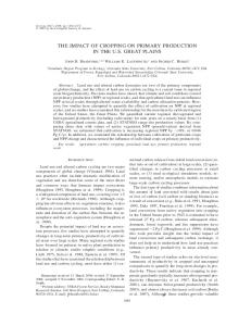
where S is entropy, Ω is the number of ways in which a particular state or configuration can occur, and κ is Boltzmann’s constant. The statistical-mechanical definition in Equation 2.1 was formulated to be consistent with a thermodynamic interpretation, hence the presence of the Boltzmann constant. The Second Law of Thermodynamics requires that an isolated system that undergoes change will always change from order (low probability state) to chaos (high probability state). Because Equation 2.1 has statistical roots, perceptions arise that the Second Law of Thermodynamics is a weak law that can theoretically be circumvented since it is not a fundamental law of nature. Such perceptions are dismissed unequivocally by the physical sciences because the statistics of large numbers produce probabilities of such certainty that they are practically exact as is demonstrated below. The statistical significance of Equation 2.1 is illustrated by considering a heads vs. tails coin-experiment, often used in statistical demonstrations. For this purpose, consider a box with the bottom filled with coins. If the box is shaken and brought to rest, the probability distribution curve of the number of heads [state] has a normal distribution with the lowest probable state being the case where all coins are in the same orientation (registering all heads or all tails). There are only two states in which all coins are in the same orientation. This becomes the least probable state. A 50% split between heads and tails has the largest number of unique combinations amongst individual coins rendering this the most probable state. Figure 2.1 was constructed by calculating the probability of 50% heads over the probability of 49% heads (P50%/P49%) for an increasing number of coins. The probability for 49% heads becomes negligibly small compared to the probability for 50% heads for a large number of coins. The calculation in Figure 2.1 was done for up to approximately 3.3 million coins. Suppose coins are placed in a highly ordered state (for example all heads) in a box and state changes are induced by shaking the box. After every state change, the expectations are to find the coins in a more probable state, which is less ordered or more chaotic. For a large number of coins, the probability of the most chaotic state is so high that it is practically guaranteed that the coins will reach a 50% split between heads and tails after a
10
few “state changes” and that no amount of successive shakes would produce a deviation from this state. 300
Log10 (P50%/P49%)
250 200 150 100 50 0 0
0.5
1
1.5
2
2.5
3
3.5
Number of coins x10^6
Figure 2.1. Probability ratio of 50% heads over 49% heads.
Working fluids like gas or liquid contain many more molecules, measured in moles where one mole contains 6.022x1026 molecules. If the equivalent of the coin experiment is performed on the degrees of freedom in a mole of gas that undergoes change, the probability that the average behaviour is defined by the most probable state approaches infinity. Although the Second Law of Thermodynamics is a function of the behaviour of individual molecules, in the case of a gas, the overwhelmingly high probability of the most likely state implies that the macro behaviour of the gas is accurately predictable. This means, for example, that a cylinder filled with gas would not spontaneously jump in one direction because its containing gas molecules adopt an ordered state such that it causes a net vector force on the walls of the cylinder. This is despite the high kinetic energy contained in the individual molecules of the gas. The statistical bases of thermodynamic systems, such as the gas example above, are founded in the concept of entropy which allows the formulation of the Second Law of Thermodynamics as follows: “If an isolated system undergoes change, it will change in such a way that its entropy increases or, at best, remains constant” (Bueche, 1986:316). The statistical basis of entropy indeed implies that the Second Law of Thermodynamics is not a fundamental law of Physics as mentioned before. Penrose gives a strong argument in its defence as a fundamental law and “... demonstrate the almost ‘mind-blowing’ precision that lies behind the vague statistical principle” (Penrose, 2005:689).
11
The properties of gas are exploited in many energy conversion processes. While the Kinetic Theory of Gas allows direct application of Equation 2.1 and serves as the basis of the physical meaning of temperature and pressure, it is impractical in engineering applications.
The theory was reformulated in terms of entropy to give a statistical-
thermodynamic equivalent, expressed as follows for a reversible thermodynamic process (Equation 2.2) (Maczek, 1998:12):
ΔS =
Q T
(2.2)
where ΔS = change in entropy, Q = heat energy, T = temperature degrees Kelvin. A reversible process is one in which a system undergoes change and return to its original state with no net change in the system or its surroundings. In this context, the Second Law of Thermodynamics is expressed in Equation 2.3. For a system that undergoes change, the entropy remains constant if the change is reversible and increases if the change is irreversible.
ΔS (total) ≥ 0
(2.3)
Mechanical work, by definition, requires vector forces that could act over a displacement. Work performed by a working fluid equates to the force, exerted by the pressure, acting over a distance equivalent to the change in the containing boundary of the fluid as expressed in Equation 2.4. W = ∫ PdV
(2.4)
where W = work, P = pressure and V = volume. Entropy in a thermodynamic context is directly related to molecular disorder in a statistical context. The total energy of a gas is the sum of kinetic and internal energies over all the individual molecules as a scalar quantity. The work potential of the energy in the gas is limited because the molecules in the gas would not move in a coherent fashion such as to produce a vector force. Such coherent movement would represent a highly ordered or low entropy state. Large-scale conversion of heat energy to mechanical work is exclusively achieved through the use a working fluid in a thermodynamic cycle. To accomplish a vector for the working
12
cycle, the system must be configured such that the working fluid alternates between states of higher and lower order (entropy). Equation 2.2 states that the entropy in a system can be changed through a process of heat exchange. If heat is withdrawn from the surroundings into the working fluid, the entropy of the working fluid is increased while the entropy of the surroundings decrease for a net change larger or equal to zero. Similarly, if heat is withdrawn from the working fluid by the surroundings, the entropy of the working fluid is decreased while the entropy of the surroundings increase for a net change larger or equal to zero. Practically, the inequality always applies because of losses. The Clausius form of the Second Law of Thermodynamics states that heat will not spontaneously flow from a cold to a hot object (Kane, 1984:228). For this reason, the process above requires a source and a sink of heat, with a temperature difference to enable heat flow through the system. Such a process is referred to as a heat engine. 2.4
Heat Engines
The alternating creation and destruction of order in the working fluid provides the work potential required for converting heat energy to mechanical work and this is the principle of a heat engine. The process requires heat flow into and out of the working fluid at the extremities of the working cycle. This principle is best illustrated by considering thermodynamic cycles such as the Carnot cycle in Figure 2.2. Sadi Carnot [1796–1832] discovered a theoretical limit in the efficiency of heat engines in 1824 when he formulated a theoretical description of an ideal reversible heat engine as shown in the diagram in Figure 2.2 (Kane, 1984:205). This cycle is referred to as the Carnot cycle.
13
Isothermal, T1 Q1 in
P a
b Adiabatic Q=0
W
Adiabatic Q=0
d c
Isothermal, T2 Q2 out
V
Figure 2.2. Carnot cycle on pressure-volume diagram. (after Kane, 1984:230)
With reference to Figure 2.2, suppose a working fluid goes through the cycle a–b–c–d–a. The shaded area represents the total work performed after completion of the cycle – consistent with Equation 2.4. Because the process is reversible, the net change in internal energy is zero and the Law of Conservation of Energy requires that the work done be equal to the net heat flow, expressed in Equation 2.5. W = Q1 - Q2
(2.5)
Heat exchange takes place along a–b and c–d such that Equation 2.2 applies, leading to the following dependencies for the working fluid: ΔS1 =
Q1 −Q2 and ΔS2 = T1 T2
The total change in entropy is zero for the assumption of reversibility leading to the following relationship: ΔSTOTAL = ΔS1 + ΔS2 = ∴
Q1 Q2 − T1 T2
Q1 T1 = Q2 T2
Defining the efficiency, μ, as the work output divided by the energy input, it follows that:
μ=
W Q1 − Q2 Q T = = 1− 2 = 1− 2 Q1 Q1 Q1 T1
(2.6)
14
Equation 2.6 represents the maximum theoretically achievable efficiency for a reversible thermodynamic cycle. Practical cycles are irreversible because of work done against dissipative forces and heat losses. The ambient temperature naturally limits the lowest sink temperature, T2, in Equation 2.6. Therefore, to increase thermal efficiency, a higher source temperature T1 is required, which implies an increase in pressure for constant volume. This combination of high temperature and pressure creates adverse conditions for engineering materials, leading for example to a phenomenon known as high temperature creep, a time-dependent mechanism that reduces the ductility of the material and eventual rupture. The efficiency barrier, expressed in Equation 2.6, applies to all heat engines. These include energy conversion processes dominated by the following applications: •
Internal combustion engines
•
Thermal processes in large-scale electricity generation from fossil fuel or nuclear
•
Gas turbines.
Equipment manufacturers in the power generation industry foresee developments in higher efficiency plant based on advanced creep-resistant materials as listed in Table 2.1 (Clauke, 2005). However, the industry vision for nickel-based plant is doubtful in light of the “forced [market] balance” (Morgan Stanley, 2005) in nickel commodities, as well as the relative scarcity of the metal and competition from other uses (USGS, 2007:112–113). Table 2.1. Expectations for material development for advanced coal fired electric power stations (Clauke, 2005). Material
Pressure [bar]
Maximum operating Overall plant temperature efficiency [°C]
[%]
Current Technology
Chrome-molybdenumvanadium
262
545
43
2010
P92
285
600
45–47
2015
Nickel based
358
700
50
The overall achievable efficiency in a working power plant is lower than the theoretical Carnot cycle efficiency because of factors such as losses and auxiliary energy consumption. Average overall energy conversion efficiency of Eskom’s coal fired energy generation plant was 34% in 2005 (Eskom, 2005:185).
15
Heat engines based on most naturally occurring temperature gradients are not practical because the relatively low temperature differences between heat sources and sinks results in low efficiencies (Equation 2.6). An example of this is the proposed Ocean Thermal Energy Conversion (OTEC) machine, which exploits the temperature difference over the first 500 to 1000 m of water depth to drive a heat engine for power generation. The maximum achievable temperature difference around the equator is ~25°C (Sørensen, 2002:466). The theoretical efficiency in OTEC is 8% for operation between 5°C and 30°C (Equation 2.6). Despite the free energy available from the natural sources, the relatively low efficiencies render such plants not cost effective currently, and may not be overall energy effective, given the large energy investment in the material and construction of the devices. There is significant scope for efficiency improvement with large potential savings in energy resources, not only in thermal electricity generation, but also in internal combustion engines. Modern diesel engines have a thermal efficiency of up to 47% compared to ~25% for spark-ignited engines (Greene and Shafer, 2003:19). The theoretical efficiency limitation of heat engines together with practical limits in engineering materials and the physical environment in which we live means that there is a limit to efficiency improvements of heat engines. These limitations need to be considered in an economic context when one deals with scarcity of heat energy, which forms 97% of energy consumption today. In this context, limitations to the scope of efficiency improvements will be considered throughout this thesis. 2.5
Direct energy conversion
Most primary energy sources are not in a form that can be directly used to perform useful work. Combustible fuels, such as fossil fuels, contain stored chemical energy that requires a conversion process to turn the chemical energy into useful work. Other uses of combustible fuel include direct combustion for space heating and cooking. Liquid fuel, such as used in internal combustion engines, has proven to be the preferred energy carrier for mobile uses, but this form of energy has undesirable attributes, such as pollution, noise and storage requirements, for stationary use.
16
Electricity is the preferred energy carrier for stationary use because it optimally overcomes most of the hazards associated with the end-use of fossil fuel. Large-scale electricity generation further eliminates the need for storage at the point of end-use because it is available on demand through transmission and distribution networks. Large-scale conversion from heat generating energy sources, such as the burning of fossil fuel in coal or gas-fired plant, or nuclear fission reactions, is achieved by generating the motive forces, required in electromagnetic conversion, from heat engines as described in Section 2.4. The Carnot efficiency limitations of heat engines can theoretically be overcome if energy can be converted directly from its primary source to electrical energy, eliminating the thermodynamic process. There are energy conversion processes, such as fuel cells, that do not use a working fluid to convert chemical energy to forms that can be used to deliver useful work and these processes are referred to as direct energy conversion devices. Chemical reactions are, however, not free from the entropy conditions of the Second Law of Thermodynamics (Equation 2.3), but limited by chemical affinities in the reaction under consideration (Fast, 1968:93). Direct energy conversion processes have only been applied commercially on a relatively small scale for energy applications or are still in research phase. These technologies in most cases are not seen as a viable substitute for fossil fuels for a number of reasons, including: •
The scale of application required for replacing heat engine applications.
•
Technological breakthroughs required to realise the theoretical efficiency advantages have proven challenging and are not guaranteed.
•
Associated technologies are material intensive leading to costly manufacturing processes, often involving scarce materials such as platinum group metals.
For these reasons, policy support institutions do not consider technologies such as fuel cells in energy projections over their planning horizons of typically 25 to 30 years (Mandil, 2006). Other direct energy conversion devices in various stages of development include the following: •
Photovoltaic
•
Thermoelectric
•
Direct conversion fission reactor.
17
There are great expectations for photovoltaic panels amongst proponents of renewable energy. Government supported programs with feed-in tariffs have led to exponential growth in manufacturing of photovoltaic capacity with associated cost benefits (Davis, 2007:34). 2.6
Energy Use
Fossil fuel dominates global energy supply, constituting more than 80% of Total Primary Energy Supply in 2004 (IEA, 2003 to 2006). Table 2.2 and Table 2.3 give a breakdown of global energy supply in percentage and tons of oil equivalent (toe) respectively. Despite concerns over greenhouse gas emissions, the share of fossil fuels has grown over the years 2002 to 2004. The annual increase in fossil fuel consumption was approximately ten times larger than the category of Other Renewable, which includes wind, solar and wave. Table 2.2. Global Total Primary Energy Supply (TPES) mix in percentage (Source: IEA, 2003 to 2006). TPES [%]
2002
2003
2004
Oil
34.9
34.4
34.3
Gas
21.2
21.2
20.9
Coal
23.5
24.4
25.1
Nuclear
6.8
6.5
6.5
Hydro
2.2
2.2
2.2
Combustible Renewable & Waste
10.9
10.8
10.6
Other Renewable
0.5
0.5
0.4
Total Fossil
79.6
80.0
80.3
18
Table 2.3. Global Total Primary Energy Supply (TPES) mix in million tons of oil equivalent (Mtoe) per year (Source: IEA, 2003 to 2006). TPES [Mtoe]
2002
2003
2004
Oil
3 570
3 639
3 793
Gas
2 169
2 243
2 311
Coal
2 404
2 581
2 776
Nuclear
696
688
719
Hydro
225
233
243
Combustible Renewable & Waste
1 115
1 143
1 172
Other Renewable
51
53
44
Total Fossil
8 143
8 463
8 880
Fossil fuel also dominates Total Final Consumption globally, constituting 66% of Total Final Consumption in 2004 (IEA, 2003 to 2006). Table 2.4 and Table 2.5 give a 2
breakdown of global Total Final Consumption in percentage and tons of oil equivalent (toe) respectively. Table 2.4. Global Total Final Consumption (TFC) mix in percentage (Source: IEA, 2003 to 2006). TFC [%]
2002
2003
2004
Oil
43.0
42.6
42.3
Gas
16.2
16.4
16.0
Coal
7.1
7.4
8.4
Electricity
16.1
16.1
16.2
Combustible Renewable & Waste
14.1
14.0
13.7
Other
3.5
3.5
3.4
Total Fossil (oil, gas, coal)
66.3
66.4
66.7
19
Table 2.5. Global Total Final Consumption (TFC) mix in million tons of oil equivalent (Mtoe) per year (Source: IEA, 2003 to 2006). TFC [Mtoe]
2002
2003
2004
Oil
3 051
3 104
3 233
Gas
1 149
1 195
1 223
Coal
504
539
642
Electricity
1 142
1 173
1 238
Combustible Renewable & Waste
1 000
1 020
1 047
Other
248
255
260
Total Fossil (oil, gas, coal)
6 202
6 302
6 461
It can be calculated from the data in Table 2.4 and Table 2.5 that only 14.8% of oil supply is converted to other forms of final consumption like electricity and non-energy use, while 76.9% of coal is converted to other forms for final consumption. The dominant use of oil is as liquid fuel in the transport sector (Table 2.6). Table 2.6. Sectoral breakdown of fossil fuel use in 2004 [Mtoe] (Source: IEA, 2003 to 2006). 2004
Oil
Gas
Coal
Industry
320
457
496
Transport
1 864
68
5
Non-Energy
543
110
28
Other*
504
587
114
* Agriculture, residential, commercial, public service and non-specific
International Energy Agency (IEA) energy statistics reflect that ~58% of oil in final consumption is used in the transport sector (IEA, 2003 to 2006). These statistics cannot be directly used to assess the impact of energy constraints on a particular sector because some indirect uses are not assigned to the economic activity of a particular sector. An example of this is that the fuel used by a sector workforce is not aggregated in the sector, but is assigned to the transport sector (IEA, 2004:27). Energy consumed in home-work-home travel is an indirect energy cost to the economic sectors because the sector would not be able to function without this energy expense. 20
Should such travel be constrained by large deviations in the availability or the price of fuel, compared to historical norms, this influence would not be accounted for in current macroeconomic modelling of the various sectors. It is important to generate statistics on homework-home travel in the different economic sectors so that it can be analysed in the context of changing energy availability paradigms. Global energy consumption patterns exhibit large variations in per capita consumption for different nations and regions (Table 2.7). The measure of kilowatt indicates the average continuous rate of consumption that includes indirect uses. If the entire world population were to use energy at the same rate as inhabitants of the OECD in 2004, it would require an increase in Total Primary Energy Supply by a factor of 2.7 (Calculated from data in IEA, 2003 to 2006). This is compared with the notional intrinsic energy that could be derived from human labour. Human power can deliver ~0.075 kW over 8 hours (or 0.3 kW for short periods) (Russwurm, 1983:19). If the total global population of 6.5 billion people had the ability to deliver power at this rate, human labour would contribute only ~1% of the 460 EJ (460*1018 J) of Total Primary Energy Supply for year 2004. Table 2.7. Average rate of energy consumption per capita expressed in kilowatt (Source: Calculated from data in IEA, 2003 to 2006).
2.7
Region
Kilowatt
OECD
6.28
Non-OECD
1.46
World
2.35
Sources of Energy
It follows from the Law of Conservation of Energy that all sources of primary energy for human consumption must be harnessed from the energy flux through the universe or from some form of stored energy. Known sources of energy are: •
Nuclear energy (fission of heavy elements and fusion of light elements).
•
Solar energy (the source of solar energy is nuclear reactions in the sun). Solar energy manifest in direct radiation as well as atmospheric circulation leading to wind, ocean currents and ocean thermal gradients.
•
Fossil fuel (solar energy captured and stored as chemical energy by biological life forms on Earth). 21
•
Geothermal energy, generally regarded as renewable.
•
Kinetic energy in the universe resulting in transient gravitational interaction between bodies. This form of energy leads to tide generating forces on Earth.
•
Chemical energy (including chemical energy derived from sunlight stored in food).
All known sources of energy flow that occur in commercially useable quantities for harnessing and consumption by humans are listed above. All these forms of energy have origins in the formation of the universe for which the most widely accepted theory is the Big Bang. Energy sources are generally divided into three categories namely: fossil,
nuclear (fission and fusion), and renewable. Technology optimism continuously challenges the presence of undiscovered sources of energy i.e. other than those listed above. It is recognised that the future is inherently uncertain and, for this reason, no definitive statements can be made regarding the probability of undiscovered sources of energy. Fundamental breakthroughs in theoretical physics would be required for the notion of undiscovered sources of energy to become a rational expectation. The breakthroughs that led to the invention of commercial nuclear energy were discovered on a physical level by Henri Becquerel [1852–1908] in 1896 (Kane, 1984:629) before Albert Einstein [1879–1955] formulated the first theoretical steps in the early 1900s. Thereafter, it took several decades before Enrico Fermi [1901–1954] produced the first controlled nuclear reaction in a reactor at the University of Chicago in 1942 (Kane, 1984:643). The energy potential of both nuclear fission and fusion were well understood and documented at the time. Thermonuclear fusion is currently the most promising unexploited source of energy, but the conditions required to yield net energy has been formulated more than a half century ago (Lawson, 1957) and despite significant research efforts, the estimated lead-time to a commercial breakthrough has remained static at ~40 to 50 years. The International Thermonuclear Experimental Reactor (ITER) project aspires to complete construction on the World’s first prototype power generation fusion reactor by 2050 in a fast track development option (ITER, 2008). There are no other known physically observable effects related to energy exchange that cannot be explained by theoretical physics. This does not exclude the possibility of
22
breakthroughs that could fundamentally change the laws of physics as formulated today, but such a breakthrough seems unlikely and should not be considered in energy planning, especially not if the notion is used to suppress emerging sustainability fears. 2.8
Conclusions and summary
The laws of physics dictate that energy cannot be created. Energy can only be harvested from natural flows (renewable) or unlocked from storage (coal, oil, gas, nuclear). The options listed in parentheses above are the only known sources of primary energy that occur at practically exploitable quantities and qualities for human utilisation. Prospects for increasing the useful energy from known fuel sources by efficiency improvements are restricted by theoretical concepts associated with the Second Law of Thermodynamics as well as by constraints in engineering materials. Although there is still significant scope for improvement in engineering materials, realistic assumptions should be considered in long-term energy planning. The fraction of fossil fuel in the Total Primary Energy Supply is dominant. This fraction has been growing, despite concerns over CO2 emissions that lead to global warming. Current levels of energy consumption are far beyond humankind’s biophysical potential. It is essential to maintain and develop non-biophysical energy sources if the current level of energy dependence is to be retained.
23
CHAPTER 3: 3.1
PEAK OIL
Introduction
This chapter deals with logistical constraints on the exploitation of exhaustible energy resources. The concept of logistical constraints is consistent with the Law of Diminishing Returns. It is logically deducted that any physical process that exhibits geometric or exponential growth must be subjected to the principle of diminishing returns at later stages to avoid physical singularities such as growth to infinity. The notion of diminishing returns is reinforced in cases where a productive process is applied to a finite quantity such that the cumulative production must converge to the finite quantity over time, regardless of the exponential growth in production that may have been encountered in the early life of the process. The cycle of accelerating and diminishing returns over time gives rise to the logistic or s-function for the production of a finite commodity. The notion that fossil fuel is a non-renewable resource leads to the conclusion that its production is subjected to a logistic function over time. This conclusion is consistent with Peak Oil theory, which describes the rise and fall of production with a peak rate of
production at the inflexion point of the logistics curve. Despite substantial empirical evidence in support of peak oil theory, the total amount of non-renewable fossil fuel resources available remains a contentious issue. Initial predictions on the limitations of fossil fuels, particular oil, were overstated (Bentley, 2002) and the reputation of such forecasts was discredited as a result. There is general agreement that oil depletion will occur before gas and coal (Campbell, 2005; BP, 2008). It is recognised today that some oil provinces have reached a peak in conventional oil production and are in a steady long-term production decline (IEA, 2006a:95). For this reason, oil is used as a leading example of fossil fuel depletion. Although the geophysical sciences have established assessment methodologies and have achieved major technological advances, reserves and resources cannot be appraised without direct access to test results and commercially sensitive information. Such information is not readily available. The only insight into reserve estimates comes from company reports as it is disclosed for investor interest. Rules for reporting reserves categories differ across the globe. In the USA
24
reporting rules are controlled by the Securities & Exchange Commission rules in order to maintain systematic statistics on energy reserves. It is uncertain whether these rules are applied consistently outside Organisation for Economic Co-operation and Development (OECD) countries. Reporting by National Oil Companies in the Organisation of the Petroleum Exporting Countries (OPEC) specifically is known not to adhere to the same reporting standards of OECD member states. This chapter gives an overview of the logistics approach applied to oil production in the lower 48 States of the USA, followed by a detailed discussion of the global peak oil debate. Although the concept of peak oil was developed for conventional crude oil, the principles apply also to other resources such as gas, coal and other minerals. 3.2
Terminology and Units
Common oil terminology is provided and is used throughout the text in the context explained below. The peak oil debate has resulted in rhetoric around oil industry definitions, apparently because of the perception that changes to the definition of terms such as conventional oil would fundamentally change the merits of certain viewpoints. For this reason, the definitions are provided in a normative context and are not meant to reflect industry consensus. •
Conventional or Regular Oil: Oil deposits that are accessible through conventional
recovery techniques. The purpose of this classification is to highlight the quality of the deposit with respect to productivity. •
Energy Profit Ratio (EPR): The ratio of energy return on energy invested in the
production of energy commodities. •
Original Oil In Place (OOIP): Total amount of oil in a reservoir before production.
•
Primary Recovery: Oil production that relies on the natural energy of the oilfield
such as the well pressure and natural water drive. •
Proven Reserves: Oil reserves that have been discovered and are considered as viable
to produce to a probability of larger or equal to 90% under prevailing economic conditions. •
Recovery Factor: The fraction of the OOIP that is recoverable. The global average recovery factor is in the range of 29% (Robelius, 2007:28) to 35% (IEA, 2005a:14).
•
Reserves: The quantities of oil that are anticipated to be commercially recoverable
from known deposits from a given date forward.
25
•
Resources: The remaining oil in place i.e. OOIP minus cumulative production.
•
Secondary Recovery: Production through use of a secondary fluid, such as gas
injection or water flooding, to maintain well pressure. •
Tertiary or Enhanced Oil Recovery (EOR): The last stage of production in the
properties of the oilfield or the oil is altered through chemical or thermal processes to enhance the flow of oil towards the wells. •
Ultimate Recoverable Reserves (URR): The total reserves that will ultimately be
produced i.e. OOIP * RF = URR. •
Unconventional Oil: Oil that cannot be produced by methods that allow production
rates equivalent to conventional oil because of its properties (solid or low-viscosity) or its location (ultra-deep water or arctic). The following units are used throughout the text: Million barrels – Mbl, Billion barrels – Gbl. 3.3
Origin of Oil
The purpose of this section is to discuss the origins of fossil fuel, as it forms part of the debate on depletion theories. The widely recognised theory is that fossil fuel has organic origins. There is school of thought that suggests that oil is formed by abiotic processes in the Earth’s mantle, from where it rises to the surface (Kenney et al., 2002). 3.3.1
Organic Origin
It is generally recognised that fossil fuels were formed from organic deposits that were laid down millions of years ago. The formation of oil, gas and coal follows different processes. A widely used hypothesis is that oil and gas are formed from organic-rich marine organisms deposited on the ocean floor (Deffeyes, 2001). Sedimentary layers of soil covered the organic-rich deposits over geological time to form the source rock for oil and gas. The sediment rich source rock is exposed to long-term geological processes that cause it to sink and rise through the Earth’s crust. Source rocks need to have been exposed to specific sequences of temperature and pressure for oil or gas to form. Oil formation takes place when source rock passes through the “oil window”, conventionally defined as being between 7 500 to 15 000 ft (2 300 to 4 600 m) below the surface. Long-term exposure to conditions in the oil window cracks the organic molecules to form shorter chains of carbon atoms with hydrogen atoms bound to the sides and ends. Such
26
molecules are referred to as hydrocarbons. If the sediments go deeper than the oil window, temperature and pressure conditions crack the hydrocarbons further to form gas. When liquid hydrocarbon is formed, it tends to migrate to the surface through porous rock formations. Most hydrocarbons are trapped in porous reservoir rocks below tight sealing cap rocks. Approximately half of known oil resources are found in sandstone reservoirs, while most of the other half occurs in limestone and dolomite (Deffeyes, 2005:16). Coal is formed from land-based plant debris that accumulated under swamp-like conditions in which plant growth exceeded decay. This caused organic-rich deposits to from. Organicrich layers of plant deposits were buried by sedimentary processes, and subsequently subjected to high pressure and temperature processes, leading to coal formation (Deffeyes, 2005:88). 3.3.2
Inorganic Origin
Professor Nikolai Kudryavtsev [1893–1971] published the modern Russian–Ukrainian theory of abiotic oil in 1951 (Kenney et al., 2002). The theory evidently has some scientific merits and it has been proven that simple molecules like methane can be formed synthetically in a laboratory under conditions resembling the outer mantle of the Earth. A detailed debate regarding inorganic origins of oil is outside the scope of this study. It is however important to interpret the significance of the debate in the context of resource depletion. Proponents of the abiotic oil theory consider the possibility that oil is a renewable resource since reservoirs are continuously replenished from large reservoirs in the Earth’s mantle (Odell, 2001). The following points are represented as critique by oil specialists in opposition to the abiotic theory as a significant factor in future oil supply: •
The evidence of production peaks and decline in many oil fields and provinces (McCann, 2001:30) indicates that the rate of replenishment is too slow to contribute significantly to reserves, if such replenishment occurs (Bardi, 2004).
•
There are some examples where abnormal reserve growth was registered including Eugene Island (Gulf of Mexico) and Ekofisk (Norway). In all known cases, the abnormal reserve growth and production profiles can be explained by geographic factors. The Eugene Island fields are connected to the source rock by one of the largest and best-known faults in the Gulf of Mexico. Ekofisk has an unusual
27
reservoir rock formation that collapsed resulting in a 7 m subsidence in the seabed (Laherrère, 2006). Examining oil production profiles of various oil fields and provinces reveals that there is in general no evidence to support significant replenishment of reservoirs as oil is extracted (Magoon, 2000). Because of this fact, the merits of the abiotic theory of oil are considered immaterial to the debate on resource depletion, and are not considered further in this thesis. 3.4
History of Oil Depletion Forecasts
Awareness of resource depletion traces back to the population problem formulated by Thomas Malthus [1766–1834] in which he raises the concern that, when left unchecked, population exhibits geometric growth and that agriculture would not be able to keep pace with such growth with obvious long-term implications. Advances in agricultural in the 20th Century (fuelled by the extensive use of fossil fuels for mechanised agriculture and artificial fertilisers) have nominally overcome these concerns. The sustainability of exponential growth in human activity has since been challenged by a number of researchers (Hardin, 1968; Meadows et al., 1972; Daly, 1980; Tainter, 1988; Duncan, 1993). Most of these studies are treated with scepticism and stigmatised as Malthusian doomsday prophesies, largely because of the inability to interpret the implications of such studies over the long time scales of relevance. These studies are becoming relevant again in public debate as the consequences emerge (UNEP, 2007). This section deals specifically with the history of oil depletion forecasts. Attempts to discredit the principles involved in peak oil theory are diminishing as the realisation that the accuracy of the forecasts of the date of peak oil are of secondary importance compared to the inevitability of eventual resource depletion. Awareness of oil depletion was first raised in a report by M King Hubbert, in which he used graphical methods to construct a logistic curve for oil production in the lower 48 States (L48) of the USA (Hubbert, 1956). Hubbert proposed a bell-shaped curve to represent the rate of oil production with time, under the assumption that the production rate will be zero at the onset of production, and again zero when the reserves are
exhausted. Hubbert assumed a symmetrical profile, which implies that peak production is reached once half the recoverable reserves have been extracted. The original curve from Hubbert’s 1956 paper is shown in Figure 3.1. (Peak Oil texts often suggest that Hubbert
28
used the discovery curve as a proxy for the production curve. This approach would be consistent with Hubbert’s work because it provides a means for estimating URR, but Hubbert did not strictly follow this approach.) Based on his most optimistic estimation of Ultimate Recoverable Reserves (URR) of conventional oil, Hubbert’s analysis suggested a peak in US L48 oil production would occur in the early 1970s. This assessment proved valid when the US L48 oil production indeed peaked in 1970 (BP, 2008). Hubbert’s approach was consistent with logistic-curve analysis.
Figure 3.1. Hubbert’s 1956 prediction of peak oil production for the L48 States. (Source: Hubbert, 1956)
This phenomenon of Peak Oil has subsequently been observed in many other oilfields and oil producing provinces and is well described by the following extract from an article in the Australian Energy News (McCann, 2001:30) that quotes United States Geological Survey
(USGS) geologist, Magoon (2000): “Production patterns are the same for oil fields, oil provinces and countries. They start out with a very rapid rise in production, reaching peak output very soon after they are commissioned. After a while production levels off and then there is a long period of declining production. This profile of production can be seen in many countries around the world already. North America, including the huge Alaskan and Mexican fields, peaked in 1984, the former Soviet Union peaked in 1987, Europe peaks this year 2001, Africa 2001, fields in the Asia Pacific region will peak in 2003, South and Central America, 2005, the Middle East in 2010.”
29
The concept of peak oil applies specifically to conventional oil. Technological progress has allowed reclassification of some unconventional resources to the conventional category, primarily because of economics. Hubbert’s theories gained acceptance when US production peaked in 1970. Hubbert’s work inspired a number of researchers to study his methodology and to make predictions for the peaking of global oil production (Bentley, 2002). Various reputable parties including the UK Department of Energy, World Energy Council, World Bank and UN made predictions through the 1970s and 1980s of a peak in global oil production around the turn of the century. Table 3.1 lists examples of more recent peak oil predictions. Knowledge of global fossil fuel resources has improved steadily since the 1970s through advances in science, extensive exploration drilling, record keeping and considerable efforts to estimate URR. Table 3.1. Historical predictions on conventional peak oil. Date
Description
Peak Year
Assumed URR [Gbl]
Reference
1977
Hubbert
1996
2000
Bentley, 2002
1998
IEA
2014
2300
IEA, 1998:100
1998
Campbell & Laherrère
2003
1800
Campbell & Laherrère, 1998:63
2000
IEA
>2020
3345
IEA, 2000:77–79
2001
Deffeyes
2004 – 2008
1800 – 2100
Deffeyes, 2001
2004
US EIA (DOE)*
2021 – 2045
2248
Wood, 2004:6
2004
US EIA (DOE)*
2030 – 2075
3003
Wood, 2004:6
2004
US EIA (DOE)*
2037 – 2112
3896
Wood, 2004:6
2004
IEA
2015 – 2035
1700 – 3200
IEA, 2004:102–103
2004
ASPO**
2008
1800 – 2000
Campbell, 2005:6
2006
IEA (OPEC)
>2030
2300
IEA, 2006a:91,93
2006
IEA (Non–OPEC)
2010
2300
IEA, 2006a:91,95
2006
CERA
2020
Not stated
2006
CERA
± 2035
2930
Jackson, 2006a Jackson, 2006b:8
* Range based on different demand growth scenarios ** Association for the Study of Peak Oil
3.5
Logistics Assessment
The bell-shaped curve, used by Hubbert, is the first derivative of a logistics or s-curve. The basic equation for the logistic function is expressed in Equation 3.1 (Bannock et al., 2003:230).
30
Q=
URR 1+e -c(t-t0 )
(
(3.1)
)
In the context of the oil production curve, Q is cumulative production, URR is the Ultimate Recoverable Reserves, t is time, to is the time associated with the inflection point where
half the URR is recovered and c is a rate dependent constant. With Equation 3.1 representing cumulative production, the first derivative of Q with respect to time represents the production rate, P, expressed in Equation 3.2. dQ URRce -c(t-t0 ) = P= 2 dt 1+e -c(t-t0 )
(
)
(3.2)
Equation 3.2 has the characteristic bell-shape of the Hubbert-curve in Figure 3.1. The production characteristics in Equations 3.1 and 3.2 can be linearised as follows. Substitution of URR from Equation 3.1 into Equation 3.2 yields: P=
ce -c(t-t0 ) Q 1+e -c(t-t0 )
(3.3)
URR -1 Q
(3.4)
(
)
It follows from Equation 3.1 that: e -c(t-t0 ) =
Substitution of Equation 3.4 into Equation 3.3 yields: ⎛ URR ⎞ c⎜ -1⎟ Q ⎝ ⎠ Q = cQ ⎛ 1- Q ⎞ P= ⎜ URR ⎟ ⎛ URR ⎞ ⎝ ⎠ ⎜ 1+ Q -1⎟ ⎝ ⎠
(3.5)
Division by Q in Equation 3.5 yields:
P c =Q+c URR Q
(3.6)
Equation 3.6 represents a linear relationship between the variables P/Q and Q and is the mathematical basis of linearised analysis such as used by Deffeyes (2001). Distortions to the linearised curve occur in the early production life. For actual production data, the ratio of P/Q for the initial time interval equals one, since P = Q for the first unit of
31
production. With increasing production, the curve becomes linear. Once the curve follows a linear relationship, a linear regression through the data points provides an approximation of URR (intercept on the Q axis) while c is the intercept on the P/Q axis. The predicted peak production would be at a cumulative production of half the URR. The methodology is demonstrated by applying it to oil production in the lower 48 states of the USA in the context of Hubbert’s 1956 assessment. A graph of P/Q vs. Q for the L48 states from 1930 onwards is shown in Figure 3.2. The production data show a discernable trend change starting from 1938 onwards. A linear regression from 1938 to 1955 projects a URR of 204.5 billion barrels (Gbl).
The production peak will thus occur when the
cumulative production reaches URR/2=102.3 Gbl. A forecast of future production is required to predict a peak date, since cumulative production in 1955 only amounted to 50.2 Gbl. An average production growth rate of 4.7% (the average for the five years from 1951 to 1955) yields a cumulative production value of 102.3 Gbl in 1970. Parameters for the 95% confidence interval of the linear regression in Figure 3.2 are listed in Table 3.2. Although the confidence intervals are symmetric around the mean values of the slope and intercept, conversion of these coefficients leads to asymmetric uncertainties around the mean URR. Applying the symmetric confidence interval to Equation 3.6 yields the ratio (URRmax-URRmean)/(URRmean-URRmin)=(Slopemin/Slopemax)~1.34 and hence the asymmetric URR interval. Table 3.2. Linear regression parameters for L-48 oil production. Estimate
Slope(-c/URR)
Intercept(c)
URR [Gbl]
t0 [year]
Minimum
-3.535E-04
6.148E-02
174
1966
Mean (R =0.75)
-3.086E-04
6.312E-02
205
1970
Maximum
-2.637E-04
6.476E-02
246
1974
Standard Error (95%)
4.492E-05
1.641E-03
-31/+41
-4/+4
2
With the values of c and URR established from the analysis in Figure 3.2, the production curve (Equation 3.2) can be constructed. The predicted production curve is superimposed on actual production data in Figure 3.3. The agreement is striking in the context of understanding URR and predicting the date of peak production.
32
0.07 Regression: P /Q = -3.09E-04*Q + 6.31E-02 0.06 URR(1955) = 50.2 Gbl 0.05
P /Q [per year]
URR/2 = 102.3 Gbl 0.04 0.03 URR = 204.5 Gbl 0.02 0.01 0 0
50
100
150
200
Q [Gbl] P/Q
Linear (1938-1955)
P/Q (Future)
Regression
Figure 3.2. Logistic curve assessment for oil production in the lower 48 states of the USA. (Source data: Campbell, 2002). “Linear” denotes the points used for the regression curve.
4
Annual Production [Gbl]
3.5 3 2.5 2 1.5 1 0.5 0 1930
1940
1950
1960
1970
Historical to 1955 Actual (1955 to 2007)
1980
1990
2000
2010
Linear (1938-1955) Logistic
Figure 3.3. Actual and modelled oil production for the US L48 states. (Source data: Campbell, 2002)
33
The scientific and deductive merits of peak oil theory are well established – the World Energy Council (WEC) endorses the methodology, declaring the ASPO (Association for the Study of Peak Oil) model as “plausible” (WEC, 2007:45–53). The methodology used in this thesis is consistent with the peak oil theory. Because the selection of the number of regression points is subjective, an analysis with an increasing number of regression points was done to demonstrate sensitivity. The result of this analysis is shown in Figure 3.4. The predictions converge as the number of regression points increases to six and beyond, despite the dynamic behaviour in the actual production
1980
300
1978
280
1976
260
1974
240
1972
220
1970
200
1968
180
1966
160
1964
140
1962
120
1960
URR [Gbl]
Peak Production Year
data.
100 0
2
4
6
8
10
12
14
16
18
Number of Regression Points Peak Year
URR
Figure 3.4. Sensitivity analysis for the number of regression points used in estimating the intercept point, URR for Figure 3.2.
Although this chapter deals primarily with oil production, application of the methodology to gas production is demonstrated for the case of Indonesia in Figure 3.5 and Figure 3.6 with units in billion cubic meters (Bcm). Linear regression parameters for Indonesian gas production (Figure 3.5) are listed in Table 3.3 for a 95% confidence interval. Table 3.3. Linear regression parameters for Indonesian gas production. Estimate
Slope(-c/URR)
Intercept(c)
URR [Bcm]
t0 [year]
Minimum
-4.622E-05
1.060E-01
2294
2002
Mean (R =0.94)
-4.204E-05
1.109E-01
2638
2004
Maximum
-3.786E-05
1.158E-01
3057
2007
Standard Error (95%)
4.180E-06
4.855E-03
-344/+420
-2/+3
2
34
Straham (2008:41) demonstrated that the same principles apply to UK coal production. Peak oil researchers adopted the use of the logistic function because it is consistent with Hubbert’s approach and because it is widely accepted in many fields of application. Alternative approaches have used Gaussian or Lorentz functions with similar results (Deffeyes, 2001:141–143). 0.3 Linear: P/Q = -4.20E-05*Q + 1.11E-01 0.25
P/Q
0.2 0.15
URR/2 = 1319 Bcm
0.1
URR = 2638 Bcm
0.05 0 0
500
1000
1500
2000
2500
3000
Q [Bcm] P/Q
Linear (1998 - 2006)
Regression
Figure 3.5. Logistic curve assessment for gas production in Indonesia.
(Source data: BP, 2008) 80
Annual Production [Bcm]
70 60 50 40 30 20 10 0 1970
1980
1990 Actual
2000
2010
Linear (1998 - 2006)
2020
2030
Logistic
Figure 3.6. Gas production trends for Indonesia.
35
(Source data: BP, 2008)
Many oilfields have asymmetric production curves unlike the perfectly symmetric profile in predicted by Equation 3.2. Figure 3.7 shows the production profiles of a sample of giant oilfields as published by Hughes (2006). Production data were obtained for the Forties field from the UK dti (2005), and for the Oseberg and Gullfaks fields from the Norwegian Petroleum Directorate (2007) for verification purposes. It is clear from Figure 3.7 that many production profiles are asymmetric to the right i.e. in the post peak regime. Peak oil researchers argue that Hubbert’s methodology is better represented if applied to discovery and production of a complete oil basin that is free of geopolitical boundaries and market imperfections (Laherrère, 2000). Laherrère and others identified a number of complicating factors, not necessarily relevant to the L48 states, in global peak oil production. Laherrère (2000) argues that global oil production is best modelled by the superposition of multiple logistic curves, each considering relevant conditions giving rise to the particular production cycle of an oil field or oil province.
Figure 3.7. Production profiles of giant oilfields, demonstrating year of peak output. (Source: Hughes, 2006)
Factors giving rise to asymmetric production curves include: •
Secondary discovery cycles
•
Quality of oil (this influences the mobility of the oil during production as well as the amount of refining required)
36
•
Quality of oil field (free flow well vs. artificial lift, improvements in extraction, location and infrastructure, pipelines, deep sea, and so on)
•
Infrastructure and export routes.
•
Enhanced oil recovery.
•
Political instability in regions.
A graph of annual production against cumulative production converges to a linear relationship in the post-peak regime (Laherrère, 2006). Estimates for the URR in the Forties field were obtained by extrapolating the curve of annual production against cumulative production to the point of zero production (Figure 3.8).
Annual Production
250 200 150 100
3090
50 0 0
500
1000
1500
2000
2500
3000
3500
Cumulative Production Production
Extrapolation
Figure 3.8. Estimation of URR for the Forties field [Mbl]. (Source of production data: UK dti, 2005)
While the representation in Figure 3.8 provides a simple means of estimating URR, it does not offer predictive information regarding the production peak or early-life estimates of URR such as provided by the logistics curve approach. Laherrère (2001, 2006) uses the representation in Figure 3.8 extensively to evaluate the influence of Enhanced Oil
Recovery (EOR) on URR. 3.6
Oil Consumption and Demand Growth
Oil demand forecasts are integrally linked to economic growth forecasts. For this reason there are a number of institutions conducting studies to forecast oil demand growth including UN, OECD, IMF. The International Energy Agency (IEA) reports the projected global oil demand growth as 1.7% per annum from 2004 to 2015 and 1.3% per annum from 2004 to 2030 in the reference scenario (IEA, 2006a:491–563). There are minor
37
discrepancies in different sources of oil consumption data and the IEA values (2006a) are understated compared to some other sources as listed in Table 3.4. Cumulative production may be taken to be equivalent to cumulative consumption, since the quantity in stockpiles is equivalent to only a few months of production. Cumulative production from 1859 to 1996 amounts to 797 Gbl (EIA, 1999:14). The BP statistical review (BP, 2008) contains oil consumption data from 1965 from which the cumulative consumption to 2003 is calculated as 989 Gbl. These values are consistent with IHSEnergy, reporting cumulative production to the end of 2003 as 1020 Bbl (Chew, 2005). Table 3.4. World oil demand in million barrels per day and cumulative consumption (historical and projected). Year
Demand (IEA, 2006a) [Mbl per day]
2003 2004
79.1
Demand (IEA, 2007) [Mbl per day]
Demand (BP, 2008)
Cumulative consumption*
[Mbl per day]
[Gbl]
79.3
78.3
1 020
82.4
80.8
1 050
2005
83.7
1 081
2006
84.5
1 112
2007
86.0
1 143
2015
95.4
1 417
2030
112.0
2 020
* Based on 2004 demand of 82.4 Mbl per day and projected growth from (IEA, 2006a) as quoted above.
The strongest component of current and projected oil demand growth is from the developing world and in particular from China (IEA, 2006a:86). Per capita oil consumption in China is 1.9 barrels per year, compared to 15 barrels per year in the OECD countries and ~26 barrels per year in the USA (IEA, 2006b; BP, 2008). China’s GDP growth is predicted to average 7.3% from 2004 to 2015 and 4.3% from 2015 to 2030 while population growth is predicted as 0.6% (IEA, 2006a:59,56). China’s rapid growing economy will raise GDP per capita and income per capita. The International Energy Agency (IEA) predicts that China’s oil demand would increase from 6.5 Mbl per day in 2004 to 8.4 Mbl per day in 2010, 10 Mbl per day in 2015 and 15 Mbl per day in 2030. Nel and Cooper (2008) demonstrate that the IEA oil demand forecast for China (IEA, 2006a) deviates substantially from historical trends. A comparison of OECD
38
projections against the same statistical data does not reveal predictions of fundamental changes in behaviour with respect to energy consumption as a function of GDP per capita. Nel and Cooper (2008) derived a logistics curve for an oil demand forecast (Figure 3.9). They noted that although their “Least Squares China” curve would predict a historically unprecedented low-growth regime in oil demand, it would be more consistent with historical trends for developing economies, compared to the IEA (2006a) forecast. The IEA (2007) has since upgraded their forecast for China from the World Energy Outlook 2006 (IEA, 2006a), but not to the extent that it significantly alter the trends in Figure 3.9. 20 18
Oil/Capita [Barrels per year]
16 14 12 10 8 6 4 2 0 0
5
10
15
20
25
30
35
40
GDP per Capita (2000$ PPP x 1000) Country Statistics (2005)
China Projections to 2030 (IEA)
China Historical
Eastern Europe
Korea
Thailand
Least Squares Gompertz
Lower Bound Gompertz
Least Squares China
G7 Historical
OECD Projections to 2030 (IEA)
Figure 3.9. Oil consumption per capita against GDP per capita. Based on 2000 USD in Purchasing Power Parity for a number of countries in 2005. Historical trends for China and projections for China are superimposed. (Source: Nel and Cooper, 2008)
Based on Nel and Cooper’s analysis (2008), China’s oil demand could be underestimated by 2, 5 and 8 Mbl per day by 2010, 2015 and 2020 respectively, given the economic growth forecasts. Assessments of oil demand forecasts for other developing economies could result in similar underestimations of future oil demand.
39
3.7
Oil Discovery
Oil discovery curves can be used as a very effective trending tool on which to base forecasts (Hubbert, 1956). It is however important that the discovery curve gives a true reflection of new finds (Campbell and Laherrère, 1998). For example, OPEC’s reserve upgrades in the 1980s (if accepted as real and not political) should not be listed as discoveries, but should be backdated to upgrade the size of the fields at the date of discovery. ASPO newsletters (Campbell, 2005) publish a backdated discovery curve, based on data from ExonMobil (Figure 3.10). Although the author could not independently trace the source of information to ExxonMobil, the graph in Figure 3.10 is also used by other institutions such as the US Department of Energy (Johnson et al., 2004:7), quoting the Oil
and Gas Journal as the source of information.
Figure 3.10. Oil discovery as reported by ASPO newsletters. (Source: Campbell, 2005)
There is no explicit knowledge regarding undiscovered oil and gas resources. The World
Petroleum Assessment project, run by the United States Geological Survey (USGS), has been the most comprehensive attempt to estimate oil and gas resources to date (USGS, 2000). The USGS study, published in year 2000, includes statistical estimations of “yet to
be discovered” reserves and makes forecasts based on 5, 50 and 95% probabilities that the reserves exist and will be discovered. The USGS results are listed in Table 3.5.
40
Table 3.5. USGS estimates of undiscovered conventional oil and natural gas liquids [Gbl]. Probability
95%
50%
5%
Mean
Conventional oil
334
607
1107
649
Natural gas liquids
95
189
478
207
Total
429
796
1585
856
The USGS (2000) estimates are widely used in scenarios for future oil supply (EIA, 2006:27–28; IEA, 2004:94; OPEC, 2007:62). If the mean estimation of undiscovered reserves (Table 3.5) were to be found by 2050, the average annual discovery would be ~19 Gbl. This would signify a significant diversion from the historical trends in Figure 3.10. Such a significant trend change is not supported by recent discovery trends, which are in the order of 10 Gbl per year (IHS Energy, 2004), nominally following the “Future Discovery” trend in Figure 3.10. IHS Energy (2004) reported that 144 Gbl of new discoveries were made from 1995 to 2003. This equates to ~16 Gbl per year or 44 million barrels per day (approximately half the demand as listed in Table 3.4). IHS Energy (2004) stated that 65% of the 2003discoveries were deep-water discoveries (in excess of 1 km water depth). These statistics are reflected in the discovery trend in Figure 3.11. The 95% USGS estimate for undiscovered reserves is 429 Gbl (Table 3.5). Discovery of 10 Gbl per year would see the discovery of all these reserves in ~50 years.
Figure 3.11. Recent oil discovery trends. (Source: IHS Energy, 2004: Figure 2)
41
The fact that oil production has exceeded oil discoveries over the last decade is also reflected in the fact that most oil produced today comes from oilfields that were discovered more than 30 years ago (Fleay, 1998). Statistics quoted by Fleay are presented in Table 3.6. With oil demand and production exceeding new discoveries, the percentages of oil production from old fields are logically set to increase. Table 3.6. Oil production by age of field (Source Fleay, 1998). Age of fields
% of current production
>20 year
90
>30 year
70
Giant oilfields are classed as fields with recoverable reserves in excess of 0.5 Gbl. This classification in itself can be misleading if one considers that the Ghawar field is estimated to have 110 Gbl of recoverable oil. Although the discovery of giant oilfields is in rapid decline IEA (2002:48), the size and quality of newly discovered fields are also in decline. The role of giant oilfields in global oil supply is depicted in Figure 3.12.
Average Field Size [Mbl]
100000 50% of all oil discovered in 53 super giant fields
10000 1000 100 10 1 10
100
1000
10000
100000
Number of Fields in Group Each grouping represents 10% of oil discovered
Figure 3.12. Distribution of all discovered oil reserves in groupings of field size on a log-log scale at end of 2003. Excludes USA and Canada. (Source data: Chew, 2005)
The 53 giant oilfields, containing 50% of all oil reserves discovered, also has a skew distribution (Figure 3.13). Simmons (2004) presents arguments in support of the notion that the distribution in Figure 3.13 is typical of regional distributions of oilfields such as for the USA and the Middle East. Assuming that the largest fields are discovered first, it
42
implies that the next “10%-equivalent” of new conventional crude oil discoveries would be in field 100 000 fields of sizes below 10 Mbl, as indicated by the broken line arrow in Figure 3.12. The logistical complexity of producing oil from an increasing number of oilfields that are geographically dispersed and of decreasing size follows logically. 160 140
Field size [Gbl]
120 100 80 60 40 20
51
46
41
36
31
26
21
16
11
6
1
0 Field Number
Figure 3.13. Field size distribution of the 53 largest oilfields that represent 50% of all discovered oil reserves. (Reproduced from Chew, 2005)
3.8
Oil Production
The historical oil production profile is characterised by geometric growth at a rate of 6.9% per year from 1900 to 1974 (calculation based on data from Campbell, 2002). This rapid growth phase is followed by a significant reduction in growth because of the subsequent oil crises (Figure 3.14). Sources of global oil production data are listed in Table 3.7. It is generally believed that the oil crises were caused primarily by geopolitical tension (Webster’s, 1992: 834; Yergin, 1991: 588–714). An alternative viewpoint is reflected in US senate hearings from 1974 to 1979 where concerns were raised that production rates from the Saudi Arabian oilfields were unsustainable, and that continued mismanagement of the fields would have led to premature decline and poor recovery (Simmons, 2005:377– 384). The author could not gain access to the transcripts referenced by Simmons (2005), but a simple extrapolation of the 6.9% growth trend leading to 1974 demonstrates the plausibility of his claims. The peak oil debate deals with the maximum achievable
43
production rate. It is currently disputed, even amongst oil optimists, whether it is plausible to achieve a production rate of 120 Mbl per day (Franssen, 2006). A production rate of 120 Mbl per day (43 Gbl per year) would have been reached by 1984 if the growth rate of 6.9% were maintained beyond 1974 (Figure 3.14). Table 3.7. Source data for global oil production. Period
Average of Sources
1900 to 1929 1930 to 1964
Data Type
Rodrigue, undated
Reproduced from graph.
Rodrigue, undated
Reproduced from graph.
Campbell, 2002
Table
Rodrigue, undated 1965 to 1970
1971 to 2006 2007
Reproduced from graph.
Campbell, 2002
Table
BP, 2008
Table
Campbell, 2002*
Table
BP, 2008
Table
BP, 2008
Table
* Data in Campbell, 2002 has projections to 2050 50 45
Annual Production [Gbl]
40 35 30 25 20 15 10 5 0 1900
1910
1920
1930
1940
Historical
1950
1960
6.94% Growth
1970
1980
1990
2000
2010
43 Gbl/year
Figure 3.14. Oil production history and scenarios related to the oil crises in the 1970s. (Source data: Table 3.7)
Recent price and oil production trends (including condensate and natural gas liquids) are shown in Figure 3.15. The data show that production has failed to respond to price
44
increases. BP (2008) records the first decline in production in recent history occurred between 2006 and 2007. 90
Price [$/barrel] Production [Million barrels/day]
80 70 60 50 40 30 20
Production
Oct-07
Oct-06
Oct-05
Oct-04
Oct-03
Oct-02
Oct-01
Oct-00
10
Price
Figure 3.15. Oil production and price trends. (Source: EIA, 2008) Price data based in international average weighted by volumes.
3.9
Oil Reserves and URR
Logistics analysis of oil production requires an estimation of the URR. Although the methodology of linearisation (Section 3.5) provides an empirical basis for estimating URR, there is still considerable disagreement regarding URR because of a number of factors including reclassification of non-conventional reserves and technology optimism for EOR to raise recovery factors in existing reservoirs. Because URR is apparently regarded as the most important parameter in the prediction of peak oil, it has become a contentious issue between oil optimists and pessimists. Both the overall URR and the quality of the reserves are relevant to the peak oil debate. Reserve quality is used here as a measure of factors that could constrain the production rate. Production of conventional oil from natural well pressure clearly requires less energy, infrastructure and processing compared to the energy intensive steam washing processes
45
involved in oil sand production. The Alberta oil sands contain an estimated 315 Gbl of URR (IEA, 2006a:97) of crude bitumen resources that would increase global URR considerably, but oil sands would not deliver the same production rate as an equivalent conventional oil field with the same URR. Peak oil deals primarily with production rates and not URR. Although some peak oil theorists focus much attention on the determination of URR from prolific conventional resources, the approach followed in the logistics assessment (Section 3.5) fully accounts for the production contributions from non-conventional reserves, increasing the URR and delaying the production peak. The estimated URR in the logistics analysis is therefore not strictly categorised in terms of reserve quality, but is rather a parameter that is representative of the production logistics. Various published results of ultimate recoverable reserves (EIA, 2000) are shown in Figure 3.16. There are only a few estimations that exceed the 95%-USGS estimate (Table 3.5), of which two are from the USGS for less certain categories.
Figure 3.16. World URR estimates. (Source: EIA, 2000)
Laherrère (2001) calculated estimates as listed in Table 3.8. The data in Table 3.8 compare well with the IEA (2004:102) low resource case. Estimates of URR are complicated by the impact of political and commercial influences on data transparency.
46
Table 3.8. URR estimates of crude oil [Gbl] (Source: Laherrère, 2001). Classification
Minimum
Mean
Maximum
Conventional oil
1700
1800
2200
Conventional gas liquids
200
250
400
Non-conventional liquids
300
700
1500
Total
2200
2750
4100
URR consists of cumulative production, proven reserves, reserve growth and undiscovered oil. Proven reserves are oil reserves that have been discovered and are considered as viable to produce to a high degree of probability under prevailing economic conditions. There seems to be reasonable agreement between different sources on remaining proven reserves (Table 3.9). Table 3.9. Remaining world proven reserves [Gbl]. Reference
Proven Reserves
Year
USGS, 2000
959
1996
CIA, 2007
1295
2005
Chew, 2005
1265
2003
BP, 2008
1208
2006
BP (2008) lists the consumption rate for 2006 as ~30 Gbl per year. At this rate, the
reserves-to-production-ratio (R/P) is 43 years based on the data in Table 3.9. Assuming that the current discovery rate of ~10 Gbl per year is maintained to 2030 and the demand listed in Table 3.4 is realised, the proven reserves would be 530 billion barrels by 2030. However, there is increasing concern about the validity of reserves booked by OPEC (IEA, 2004:92) given the increase in reserves claimed in the early 1980s. Most OPEC countries made major adjustments to their proven reserves in the 1980s (Table 3.10) without significant known discoveries. These reserve updates were driven by negotiations over production quotas and were considered political at the time, with no contributions from actual discoveries (IEA, 2004:92).
47
Table 3.10. Single year increases in OPEC reserves [Gbl] (Source: BP, 2008). Year
Iran
Iraq
Kuwait
Saudi Arabia
Venezuela
1980
58.30
30.00
67.93
168.03
19.53
1981
57.02
32.00
67.73
167.85
19.89
1982
56.15
59.00
67.15
165.48
24.90
1983
55.26
65.00
67.00
168.85
25.89
1984
58.87
65.00
92.71
171.71
28.03
1985
59.00
65.00
92.46
171.49
54.45
1986
92.86
72.00
94.52
169.74
55.52
1987
92.86
100.00
94.53
169.59
58.10
1988
92.86
100.00
94.53
254.99
58.51
1989
92.86
100.00
97.13
260.05
59.04
1990
92.85
100.00
97.03
260.34
60.05
1991
92.86
100.00
96.50
260.94
62.65
An assessment of production data against URR provides some insights to the extent by which OPEC reserves could be overstated. The achievable production rate is governed by many physical parameters related to oilfields including well pressure and permeability. Production strategies in an oilfield can be optimised for peak production or maximum ultimate recovery i.e. aggressive production techniques may result in less ultimate recovery (Frick, 1962:33.20–33.24). 4
A logistics curve approach to oil production implies a limit to the achievable production rate that depends on both the URR and geology of the oil field or province. Many factors could distort production dynamics including: •
Oil field management strategy – aggressive production could reduce the URR in a field or province (Frick, 1962:33.20–33.24).
•
Secondary discovery cycles.
•
Geological differences between fields (Frick, 1962:33.20–33.24).
•
Incorrect URR claims.
Table 3.11 and Table 3.12 were compiled from data in the public domain.
48
Table 3.11. Oil production statistics for OPEC countries (Source data: Average of BP, 2008; ASPO newsletters (2003 to 2007) and OPEC, 2006). Country
Year
Cumulative [Gbl]
URR [Gbl]
Production [Gbl per Year]*
Algeria
2003
12.5
27.4
0.622
Angola
2003
5.0
13.8
0.332
Indonesia
2005
20.9
26.5
0.572
Iran
2002
54.0
165.8
1.867
Iraq
2001
27.0
140.0
0.837
Kuwait
2002
35.0
134.2
1.029
Kuwait**
2002
35.0
83.0
1.029
Libya
2002
23.0
58.0
0.865
Nigeria
2002
22.4
58.84
0.835
Qatar
2005
8.0
22.84
0.323
Saudi Arabia
2005
104.0
340.6
3.586
Venezuela
2005
41.0
129.0
1.275
* Maximum of 10-year moving average from BP (2008) ** See explanation for alternative URR for Kuwait below.
Petroleum Intelligence Weekly (PIW, 2006) reported on the contents of an internal report of the Kuwait Oil Company (KOC, the upstream arm of the Kuwait Petroleum Corporation), based on the findings of its Reserve Management Committee. According to the PIW report, the KOC report reflects reserves of 48 Gbl of which only 24 Gbl were proven. The official KOC remaining reserves in 2006 were 101 Gbl (OPEC, 2006). After initially refuting the PIW claims, Kuwait Petroleum Corporation (KPC) CEO, Hani Hussein, tendered his resignation in April 2007. His successor, Sheikh Ali Al–Jarrah Al– Sabah confirmed the accuracy of the PIW report, but claimed that Kuwait has additional probable reserves of 150 Gbl that will be developed with the aid of international oil companies (Kuwait Times, 2007) (Al-Sabah resigned in June 2007). The USGS (2000) mean estimate for undiscovered oil in Kuwait, generally considered optimistic, is three Gbl in comparison. ASPO (2008) newsletters report a URR of 83 Gbl, which is consistent with the PIW (2006) report. This latter figure was used as an alternative in Table 3.12.
49
Table 3.12. Oil production statistics for Non-OPEC countries (Source data: Average of BP, 2008; ASPO newsletters (2003 to 2007) and OPEC, 2006). Country
Year
Cumulative
URR
Production
[Gbl]
[Gbl]
[Gbl per Year]*
Argentina
2002
8.30
11.40
0.300
Australia
2002
5.80
11.30
0.243
Brazil**
2002
6.50
21.05
0.501
Canada
2003
19.16
35.90
1.036
China
2003
29.80
53.05
1.231
Denmark
2003
1.47
2.78
0.121
Egypt
2002
8.70
12.25
0.330
India
2004
6.10
12.05
0.290
Malaysia
2004
5.90
10.40
0.278
Mexico
2002
23.0
47.10
1.310
Norway
2001
16.3
29.95
1.179
Oman
2003
7.30
13.55
0.327
Russia
2002
121.0
200.0
3.564
UK
2005
22.0
29.05
0.965
USA
2001
169.0
197.20
3.885
* Maximum of 10-year moving average from BP (2008) ** Includes deep water.
The data in Table 3.11 and Table 3.12 were used to construct the graph in Figure 3.17. The ratio of URR to the maximum production rate on a ten-year moving average, denoted Max(10), is used as an index of the degree to which countries exploit their oil reserves. Defining the exploitation index as EI = {URR/Max(10)}, a relatively high value for EI would indicate that the oil reserves is relatively under-exploited in a particular country or alternatively that the URR for the country is overstated. The ratio of cumulative production to URR is used as a measure of depletion, denoted as the depletion index: DI = Q/URR. A graph of DI against EI provides a comparative view between oil producing countries (Figure 3.17). Differences in production trends between non-OPEC and OPEC countries (with large political increases in oil reserves – Table 3.10) are apparent. Kuwait’s position on the graph would be more consistent with non-OPEC producers if the corrections to its URR, discussed above and plotted as “Kuwait**”, are taken into account.
50
180 Iraq
160
Kuwait
Exploitation Index
140 120
Venezuela
100
Saudi Arabia Iran Kuwait* Qatar Libya Nigeria
80 60 40
Algeria
Indonesia
Angola
20 0 0
0.1
0.2
0.3
0.4
0.5
0.6
0.7
0.8
0.9
Depletion Index OPEC Middle East
OPEC Africa
Kuwait
Indonesia
Venezuela
Non OPEC
Figure 3.17. Comparative statistics of exploitation index (EI) against depletion index (DI) for oil producing countries. (See Table 3.11 for adjusted Kuwait values)
The phenomenon of reserve growth is common in most oilfields (Schmoker et al., 2001). The size of an oil field is first estimated based on geological and exploration information at the time of discovery. As the field is developed and produced, the trend is that the initial estimates are conservative and the size of the field is upgraded to reflect the updated estimates. Reserve growth is used in this context by the USGS (2000). USGS considers three contributions to reserve growth (Schmoker et al., 2001) namely: •
Expansion of reserves in place through area expansion of fields.
•
Expansion of reserves in place through the discovery of new pools.
•
Revisions of reserve calculations based on experience gained through operation of a field leading to higher recovery factors.
The USGS (1998:6) uses a modified Arrington method to model reserve growth. The modified Arrington method calculates a cumulative growth function (CGF) that gives the ratio of URR divided by estimated reserves at the time of discovery (Equation 3.7). (Significant figures are given as reported in the source document.)
CGF = 1.75752 ( years since discovery )
0.3005
(3.7)
51
The Securities & Exchange Commission rules have reserve categories as follows (SPE, 2007): •
Proven reserves require a 90% probability of being recoverable.
•
Probable reserves have a 50% probability of being recoverable.
•
Possible reserves should have a probability of at least 10% of being recoverable.
Not all countries subscribe to these definitions. There is great uncertainty with regards to reserves reporting for the world outside the USA as is evident in the concerns expressed by the increases in reported OPEC reserves in the 1980s (IEA, 2004:92). The OPEC reserve increases in Table 3.10 could be political, or alternatively they could be a calculated revision based on a redefinition of proven reserves to include probable and possible categories. Without the aid of a comprehensive database of field data it is, however, not possible to correlate the figures with a growth function such as Equation 3.7. The mean USGS reserve growth, as used by the IEA (2004:94), equates to 730 Gbl from a proven remaining reserve base of 959 Gbl. Enhanced Oil Recovery (EOR) techniques are employed with the aim to increase the URR
and to increase the production rate (IEA, 2005b:16). EOR makes use of thermal, gas and chemical injection techniques to enhance the mobility of oil that would otherwise not be recovered. Laherrère (2001, 2006) gives a number of examples to demonstrate that EOR does not necessarily lead to increases in URR. As an example, data from the Auk oilfield are shown in Figure 3.18.
52
20 18
Annual production [Mbl/year]
16 14 12 10 8 6 EOR
URR
4 2 0 0
20
40
60
80
100
120
140
160
Cumulative production [Mbl]
Figure 3.18. Auk oilfield, UK, production history. (Source: UK dti, 2005)
3.10 Oil Scenarios
There are two schools of thought on the oil outlook into the future: •
The EIA, IEA and CERA dominate the optimist viewpoint. These organisations serve as the main source of analytical input to political and economic forums.
•
Associations with Collin Campbell and Jean Laherrère dominate the pessimist viewpoint and claim to represent a scientific viewpoint.
3.10.1 Oil Optimism
With the acknowledgement that non-OPEC oil producers are approaching peak output (IEA, 2006a:95; EIA, 2008), the focus has turned to OPEC to increase production in order to meet increasing demand (Table 3.13).
53
Table 3.13. EIA and IEA supply projections [Mbl per day]. Country
BP, 2008 2005
2006
Non-Conventional**
EIA, 2008
IEA, 2006a:92
2015
2030
2015
2030
5.8
10.5
4.5
8.9
Iran
4.268
4.343
4.3
5.0
5.0
6.3
Iraq
1.833
1.999
3.3
5.3
2.8
6.0
Kuwait
2.643
2.704
3.2
4.1
2.8
4.0
Saudi Arabia
11.114
10.859
9.4
16.4
13.3
17.3
Algeria
2.016
2.005
2.8
3.1
2.0
1.4
Libya
1.751
1.835
2.0
1.9
1.9
2.7
Nigeria
2.580
2.460
4.5
5.2
2.7
3.2
Indonesia
1.129
1.071
1.0
0.7
0.8
0.8
Venezuela
2.937
2.824
2.8
3.3
2.8
3.9
OPEC TOTAL
34.068
34.202
37.6
50.1
41.2
54.8
Mexico
3.760
3.683
3.0
3.5
3.1
3.0
Non-OPEC TOTAL
47.183
47.462
54.0
57.1
51.3
50.2
World TOTAL
81.250
81.663
97.4
117.7
97.0
113.9
11
* Natural gas liquids are considered as conventional oil in this assessment. OPEC11 excludes Angola
There are many inconsistencies between the projections in Table 3.13 and country specific developments including: Kuwait:
The case of Kuwait’s reserve estimations was discussed in Section 3.9. In addition to Kuwait’s inflated reserves, the CEO of KPC informed Bloomberg that production from the Burgan field would reach ~1.7 Mbl per day and that they cannot maintain 1.9 Mbl per day implying that Burgan is past its peak (Cooper, 2005). Burgan has been in production for almost 60 years and accounts for more than half of Kuwait’s production.
Saudi Arabia: Saudi Aramco published their Fifty Year Crude Oil Scenarios (Baqi and Saleri, 2004) in which it claims that it is viable to increase production to 12 Mbl per day by 2016 and maintain this capacity to 2033 without relying on reserve replacement. Although there is mention of a possible 15 Mbl per day, this level of production requires the company to utilise 68% of its probable and possible reserves. Both the EIA and IEA projections, Table 3.13, are higher than Saudi Aramco’s outlook.
54
There are other discrepancies related to Saudi Aramco. Saudi Aramco Senior Vice-President of Exploration and Producing (Al-Saif, 2005) reported an
“ambitious” plan to expand the company’s production capabilities. The plan aspires to an expansion of 2.3 Mbl per day in production capacity from March 2005 to 2009, an addition of ~0.6 Mbl per day each year. Saudi Aramco estimated a natural rate in production decline of 6% per annum (~0.6 Mbl per day) from 2004 to 2009 (IEA, 2004:111). Al-Saif’s (2005) “ambitious” plans would therefore replace the declining production of existing fields with zero net gains in production. Mexico:
After production from the Cantarell oilfield, which accounts for 60% of Mexico’s oil production, unexpectedly peaked in 2005 production declines are more rapid than initially thought (Rubin and Buchanan, 2007).
Figure 3.19. Production data for Cantarell. (Source: Rubin & Buchanan, 2007)
The oil production projections listed in Table 3.13 provide no information to explain discrepancies in the production outlook such as listed above. The IEA’s World Energy Outlook series serves as a prominent institutional guideline for energy and economic planning, yet it contains elements of deception. IEA (2004:101) published Figure 3.20 as a demonstration of how technological improvements can increase production, using the Kingfisher oilfield in the North Sea as an example.
55
Annual production data, obtained from the UK Department of Trade and Industry, are presented in Figure 3.21 for comparison. The gains from the Kingfisher field were clearly insignificant, and may have resulted in a decrease in URR. URR convergence is represented by the dotted line in Figure 3.21.
Figure 3.20. Oil production from the Kingfisher field. (Source: IEA, 2004) 12 1998
Annual production [Mbl/year]
10 2001 8 1999 6 2000
2002
4 2003 2 2004
1997 0 0
10
20
30
40
50
Cumulative production [Mbl]
Figure 3.21. Oil production from Kingfisher. (Source data: http://www.dti.gov.uk/)
56
Cambridge Energy Research Associates (CERA) has received periodic attention in the media for its optimistic oil outlook. As with other optimistic outlooks, CERA communications are also marred with discrepancies. In February 2006 Jackson (2006a) said that CERA anticipates an inflection point in world oil production followed by an undulating plateau by 2020. Jackson’s projection came under scrutiny from Ward (2006), CERA Director for Upstream Technology, challenging their assumptions regarding offshore production. Notwithstanding Ward’s concern, Jackson (2006b) produced a report in November 2006 that predicts the undulating plateau in world oil production (including unconventional oil) to occur by 2035, deferred by 15 years from his earlier prediction in the same year. 3.10.2 Oil Pessimism
The most prominent depletion model is the ASPO (2008) model, presented in Figure 3.22. ASPO received institutional recognition in 2007 when the WEC (2007:45–53) endorsed the basic methodologies used by ASPO, declaring the model in Figure 3.22 as “plausible”.
Peak Oil
Figure 3.22. ASPO model for oil depletion (2005 Base Case). (Source: ASPO, 2008)
Peak oil has gained support from a number of institutions and oil executives over the last few years including Deutsche Bank Research (2004), French Government (2004), World Energy Council (WEC, 2007) and Shell (van der Veer, 2008).
57
The French Government (2004) commissioned work to evaluate the oil industry. The report provides different peak oil scenarios (Table 3.14 reproduced from a report). IEA (2007) forecasts global oil product demand to expand by 2.2% to 2012, some of which will come from unconventional sources. A demand growth of 2% and a discovery rate of 10 Gbl per year predict the peak production to occur in 2016, at a rate of 98 Mbl per day (Table 3.14). This interpretation of a possible peak date compares well with the ASPO model in Figure 3.22. Discovery data in Figure 3.10 and Figure 3.11 were digitised and reproduced in Figure 3.23 with the discovery scenarios from the French Government (2004) report superimposed. The 10 Gbl per year discovery case represents a plausible extrapolation of historical trends compared to the 20 and 30 Gbl per year scenarios (Figure 3.23). 60
40
30
20
10
ASPO (Fig. 2.4.8)
IHS (Fig. 2.4.9)
10 Gbl/year
20 Gbl/year
2050
2045
2040
2035
2030
2025
2020
2015
2010
2005
2000
1995
1990
1985
1980
1975
1970
1965
1960
1955
1950
1945
1940
1935
0
1930
Annual Discovery [Gbl]
50
30 Gbl/year
Figure 3.23. Historical oil discovery trends. (Source data: Figure 3.10 and Figure 3.11) Note that the IHS data include offshore and deep-water discoveries.
58
Table 3.14. Peak oil production scenarios based on a decline rate of 3% in existing capacity with a base year of 2005. (Source: French Government, 2004). Discoveries* [Gbl per year]
0
Demand Growth Year [%]
10
20
Consumption [Mbl per day]
Year
Consumption [Mbl per day]
Year
Consumption [Mbl per day]
0.0%
2020
79
2032
79
2054
79
0.5%
2016
88
2021
93
2033
104
1.5%
2014
91
2018
96
2027
110
2.0%
2013
93
2016
98
2023
113
2.5%
2013
96
2015
101
2020
114
3.0%
2012
97
2013
100
2017
113
* Assumption: Steady discovery rate to 2015 with 2% per annum decline thereafter.
3.11 Summary and Conclusions
Hubbert’s (1956) assessment of peak oil for the L48 States in the USA was based on sound logical principles. The inconvenient truth (after Gore, 2006) of his projections was met with resistance from authorities who applied pressure on him to withdraw his presentation (Deffeyes, 2001). Hubbert’s irrefutable logic of a bell-shaped curve for the production of an exhaustible resource coupled with best estimates of Ultimate Recoverable Reserves prevailed when oil production in the L48 States did indeed peak in 1970. In this chapter, Hubbert’s graphical methods are mathematically formulated to establish a deterministic methodology for the calculation of production logistics i.e. Ultimate Recoverable Reserves and the date of the peak production. When applied in Hubert’s
original 1956 data set, the logistics analysis methodology reproduces Hubbert’s graphically determined result accurately. Although the logic of a bell-shaped production curve is the same for all exhaustible resources, the validity of the logistics analysis was also demonstrated for gas production for a case study in which peak production has passed – the Indonesian gas fields. Analyses for global oil production, carried out by the peak oil proponent groups e.g. ASPO, predict a peak in production within the next decade. As was the case with Hubbert in 1956, such forecasts are met with resistance because it of the challenges it presents for the global economy and policy makers. A comprehensive assessment of global oil production reveals numerous inconsistencies in the views of oil optimists, with many
59
issues in the public domain left unexplained, and supports the conclusions of peak oil theory that a peak in global oil production is imminent. In light of the above, logistics analysis is accepted as a valid and plausible methodology. In Chapter 4, a logistics analysis is applied to fossil fuel commodities to derive an Energy Reference Case, which represents a probable energy future based on realistic, quantitative estimates of constrained extraction of geological energy resources.
60
CHAPTER 4: 4.1
ENERGY FUTURES
Introduction
The phenomenon of peak oil was discussed in Chapter 3 together with assessment methodologies and empirical evidence. This logistics assessment methodology, developed in Chapter 3, is expanded in this chapter to derive an Energy Reference Case. The Energy Reference Case serves as a rationally calculated benchmark for the future availability of energy resources, using the best available knowledge and empirical evidence, as imbedded in the logistics assessment methodology. The Energy Reference Case includes all known sources of energy, namely fossil fuels (oil, gas and coal), nuclear and renewable energy, as identified in Chapter 2. The Energy Reference Case is developed as follows. Historical production data are used to performing logistic curve assessments for all fossil fuel sources. Numerical values for the parameters (URR, t0 and c) of the logistics production function (Equation 3.2) are derived from the linearised logistics curve assessments, forming the bases of future production in the Energy Reference Case. Contributions from nuclear and renewable energy to the Energy Reference Case are analysed by considering fundamental scientific principles and institutional knowledge and expectations from these sources. Long-term structural scarcities in energy commodities have not been encountered in modern history. Energy prices have escalated substantially over the last few years and some researchers attribute price escalations to the imminence of peak oil (ASPO, 2008). The impacts of high energy-prices have resulted in global inflationary pressure and public unrest in some countries. It is becoming increasingly important to come to terms with plausible energy futures in long-term economic and resource planning. The Energy Reference Case is applied in later chapters to derive impacts on sustainability concerns such as global warming and socio-economic welfare. 4.2
Oil Futures
The input data for the global oil production are production statistics, from sources listed in Table 4.1. Averages are used where more than one source is available. The production data were used to construct the linearised logistics curve (Figure 4.1).
61
Table 4.1. Data sources for global oil production. Period
Average of Sources
1900 to 1929 1930 to 1964
Data Type
Rodrigue, undated
Reproduced from graph.
Rodrigue, undated
Reproduced from graph.
Campbell, 2002
Table
Rodrigue, undated 1965 to 1970
1971 to 2007
Reproduced from graph.
Campbell, 2002
Table
BP, 2008
Table
Campbell, 2002*
Table
BP, 2008
Table
* Data in Campbell, 2002 has projections to 2050
With reference to Figure 4.1, the cumulative production to 2006 is 1 132 Gbl. Assuming that future production will meet consumption, the IEA (2007) projections, extrapolated to 2014 at an annual growth of 2%, predicts that cumulative production will reach URR/2 = 1 341 Gbl by 2014. Proven reserves in 2006 are calculated as: Proven Reserves = URR - Q2006 = 2 682 - 1 132 = 1 550 Gbl where Q2006 is the cumulative production in year 2006. In comparison, BP (2008) reported reserves of 1 208 Gbl for 2006 – the predicted remaining reserves are 28% higher than reported reserves. The regression curve in Figure 4.1 provides all the variables required for the logistics production function for global oil (Equation 4.1) P=
2682 * 0.0446 * e-0.0446( t -2014)
(
1 + e-0.0446( t -2014)
)
(4.1)
2
where P is the annual production in Gbl per year. Linear regression parameters for global oil production (Figure 4.1) are listed in Table 4.2 for a 95% confidence interval. Table 4.2. Linear regression parameters for global oil production. Estimate
Slope(-c/URR)
Intercept(c)
URR [Gbl]
t0 [year]
Minimum
-1.764E-05
4.366E-02
2475
2010
Mean (R =0.95)
-1.662E-05
4.458E-02
2682
2013
Maximum
-1.560E-05
4.550E-02
2916
2018
Standard Error (95%)
1.018E-06
9.206E-04
-207/+234
-3/+5
2
The global production model prediction is shown superimposed on actual production data in Figure 4.2. The production function smoothes out the perturbations of the oil crises in
62
the 1970s. ASPO’s Peak Oil analysis is based on the aggregation of detailed country-level assessments (Campbell, 2002) that are considered more accurate than the integrated approach used here. The ASPO model includes non-conventional oil, such as Venezuelan heavy crude and Canadian oil sands (Campbell, 2002), with values that are nominally comparable to those projected by institutional authorities (IEA, 2006:92–93). 0.08 Linear: P/Q = -1.66E-05*Q + 4.46E-02 0.07 Cumulative Production (2006) = 1132 Gbl
P/Q [per year] .
0.06 0.05 URR/2 = 1341 Gbl 0.04 0.03 0.02
URR = 2682 Gbl
0.01 0 0
500
1000
1500
2000
2500
3000
Q [Gbl] Historical
Linear (1991 - 2006)
Regression
Figure 4.1. Logistic curve assessment for global oil production. (Source data: Table 4.1)
The logistic curve predictions are considered adequately representative of long-term production trends and sufficiently robust for the determination of global warming and economic impacts. Two cases are relevant to future oil production namely (i) the ASPO model and (ii) the logistics curve in Equation 4.1. Values for historical and future oil production are listed in Table A.7.1 to Table A.7.4, Appendix A, in terms of barrels and energy units in EJ (1018 J). Conversion to energy units is done by considering one barrel of oil = 5.729 GJ (BP, 2008).
63
35
Annual Production [Gbl]
30 25 20 15 10 5 0 1900 1910 1920 1930 1940 1950 1960 1970 1980 1990 2000 2010 2020 2030 2040 2050 Historical
Logistic
Linear (1991 - 2006)
ASPO (Campbell, 2002)
Figure 4.2. Global oil Production trends and projections. (Source data: Table 4.1)
4.3
Gas Futures
Sources for global gas production data are listed in Table 4.3. The production data were used to construct the linearised logistics curve (Figure 4.3), with units in trillion cubic meters (Tcm). Table 4.3. Data sources for global gas production. Period
Sources
Data Type
1930 to 1969
Campbell, 2002*
Table
1970 to 2007
BP, 2008
Table
* Data in Campbell, 2002 has projections to 2050
The cumulative production to 2006, Q2006, is 84 Tcm. Future gas production is assumed to grow at the same rate as the average rate of the five years preceding 2006. At this rate, cumulative production would reach URR/2 = 162 Tcm by 2027. However, demand growth for gas could accelerate after Peak Oil occurs. With reference to Figure 4.3, the remaining proven reserves in 2006 would be: Proven Reserves = URR - Q2006 = 324 – 84 = 240 Tcm, compared to an official value of 181 Tcm reported by BP (2008) – the predicted reserves are 33% higher than reported reserves. The logistics curve in Equation 4.2, superimposed on actual production data and ASPO projections, is shown in Figure 4.4. Parameter values
64
for Equation 4.2 were derived from the linear regression in Figure 4.3. Production units in Equation 4.2 are in Tcm. P=
324 * 0.0454 * e-0.0454( t -2027)
(1 + e
-0.0454( t -2027)
)
(4.2)
2
Linear regression parameters for global gas production (Figure 4.3) are listed in Table 4.4 for a 95% confidence interval. Table 4.4. Linear regression parameters for global gas production. Estimate
Slope(-c/URR)
Intercept(c)
URR [Tcm]
t0 [year]
Minimum
-1.549E-07
4.434E-02
286
2022
Mean (R =0.90)
-1.398E-07
4.540E-02
324
2027
Maximum
-1.246E-07
4.646E-02
373
2032
Standard Error (95%)
1.513E-08
1.059E-03
-38/+42
-5/+5
2
As for the case of oil, both the ASPO model and logistics curve assessments are considered relevant to the future production of gas. Values for historical and future gas production are listed (Table A.7.5 to Table A.7.8) in terms of Tcm and energy units in EJ (1018 J). Conversion to energy units considering one cubic meter of gas as equivalent to 36 MJ (BP, 2008). 0.1
Linear: P/Q = -1.40E-07*Q + 4.54E-02
0.09 0.08 0.07
Cumulative Production (2006) = 84 Tcm
P/Q
0.06 0.05
URR/2 = 162 Tcm
0.04 0.03
URR = 324 Tcm
0.02 0.01 0 0
50
100
150
200
250
300
350
Q [Tcm] P/Q
Linear (1996 to 2006)
Regression
Figure 4.3. Logistic curve assessment for global gas production. (Source data: Table 4.3)
65
4.5
Annual Production [Tcm]
4.0 3.5 3.0 2.5 2.0 1.5 1.0 0.5 0.0 1930
1950
Historical
1970
1990
Linear (1996 to 2006)
2010 Logistic
2030
2050
ASPO (Campbell, 2002)
Figure 4.4. Global gas production trends and projections. (Source data: Table 4.3)
4.4
Coal Futures
Sources for global coal production data are listed in Table 4.5. Coal production is measured in millions of tons (Mt) and billions of tons (Gt). Table 4.5. Data sources for global coal production. Period
Sources
Data Type
1820 to 1953
Hubbert, 1956
Reproduced from graph.
1954 to 1980
IEA, 2003
1981 to 2007
BP, 2008
Data listed in table for hard coal production. Values for total coal production in this date range were estimated by growing the 1953 value by the same annual percentages as hard coal production. Table
Table 4.6 lists the global coal reserves for different categories of coal. Differences in values between sources are the consequence of poor data quality and differences in classification (WEC, 2007). Reserves declined from 935 Gt in 2001 to 847 Gt in 2005 (production was only 26 Gt) because of refinements in the categorisation of reserves and not as a result of revisions (WEC, 2007). Despite this downward adjustment in reserves, recent trends in production show notable increases from 2002 (Figure 4.5).
66
7000
Coal Production [Mt]
6000 5000 4000 3000 2000 1000 0 1960
1970
1980
1990
2000
2010
Figure 4.5. Recent trends in coal production. (Source data: BP, 2008)
Table 4.6. Coal reserves and production data [Mt]. Proved Recoverable Reserves Source Year
Hard Coal
Brown Coal
Production
Total
Year
Hard Coal
Brown Coal
Total
WEC (2001)
2000
519 062 465 391
984 453
1999
3 011
1 332
4 343
WEC (2007)
2005
430 896 416 592
847 488
2005
4 445
1 456
5 901
The linearised logistic curve assessment for global coal production is presented in Figure 4.6. The regression curve yields a URR of 1 671 Gt. Cumulative production to 2006, Q2006, equates to 285 Gt. With reference to Figure 4.6, the remaining proven reserves in 2006 would be: Proven Reserves = URR - Q2006 = 1 671 – 285 = 1 386 Gt which is 64% higher than the reported value of 847 Gt (Table 4.6). This scenario is referenced as Coal Plus. Linear regression parameters for global coal production (Figure 4.6) are listed in Table 4.7 for a 90% confidence interval. Note that the approach followed is based on structural dependencies (not on statistical empiricism) and the low regression coefficient is primarily indicative of the volatility in coal production. A 95% confidence interval produces
67
inconsistent results (positive slope for the maximum estimate), hence the error estimation at a 90% confidence interval. Table 4.7. Linear regression parameters for global coal production. Estimate
Slope(-c/URR)
Intercept(c)
URR [Gt]
t0 [year]
Minimum
-1.745E-08
2.339E-02
1340
2059
Mean (R =0.29)
-1.434E-08
2.396E-02
1671
2071
Maximum
-1.123E-08
2.452E-02
2184
2087
Standard Error (90%)
3.112E-09
5.640E-04
-330/+513
-12/+16
2
0.03 Cumulative Production (2006) = 285 Gt 0.025 P/Q [per year]
Average: P/Q = -1.75E-08*Q + 2.44E-02 0.02 URR/2 = 700 Gt 0.015 0.01 URR = 1400 Gt 0.005 0 0
200
400
600
800
1000
1200
1400
1600
1800
Q [Gt] Historical Regression [1671 Gt]
Linear (1952 to 2006) Average [1401 Gt]
Proven [1126 Gt]
Figure 4.6. Logistic curve assessment for global coal production. (Source data: Table 4.5)
It is likely that the rapid increases in production since 2002, considered as unsustainable (Figure 4.5), have distorted the production logistics for coal causing an upward bias in the regression curve. For this reason, an alternative case (Coal Reference) is considered for the coal contribution to the Energy Reference Case. Coal Reference is based on the average between the Regression [1671 Gt] and the Proven [1126 Gt] curves (Figure 4.6). The Proven [1126 Gt] curve was constructed by forcing the linear regression fit through a URR prediction of 1126 Gt (the sum of reported
68
proven reserves and cumulative production for 2006). The average between this curve and the regression curve yields URR of 1 400 Gt – 32% higher than reported reserves. Three cases of global coal production, superimposed on the actual production data, are shown in Figure 4.7. The three cases correspond to (i) the linear regression curve (Coal Plus); (ii) a URR of 1126 Gt (to correspond to the official remaining reserves of 847 Gt
(Table 4.6); and (iii) the average between these two curves (Coal Reference).
12000
Annual Production [Mt]
10000 8000 6000 4000 2000 0 1850
1900
1950
Actual Average (ERC) [1400 Gt]
2000
Linear (1952 to 2006) Regression [1671 Gt]
2050
2100
Proven [1126 Gt]
Figure 4.7. Global coal production trends and projections. (Source data: Table 4.5)
Two cases are considered for future production of coal namely the Coal Reference (Equation 4.3) and Coal Plus (Equation 4.3) with production units in Gt per year. The Coal Reference
and
Coal Plus
cases
correspond
to
Average (ERC) [1 400 Gt]
and
Regression [1 671 Gt] respectively in Figure 4.7. PRef =
1400 * 0.0243* e-0.0243( t -2061)
PPlus =
(
1 + e-0.0243( t -2061)
)
2
1671* 0.024 * e-0.024( t -2071)
(
1 + e-0.024( t -2071)
)
2
(4.3)
(4.4)
69
Coal production statistics are generally reported in tons delivered, which include the mass of non-combustible material. The energy-based projection of coal consumption has to be adjusted to compensate for declining coal quality. In the USA, there has been a decline of ~3.6% per decade in energy content of coal throughout the second half of the 20th Century (Figure 4.8). 7.5
31
7.3
6.9
28
6.7
27
6.5 6.3
26
-1
7.1
29
Mcal kg
MJ kg
-1
30
6.1 25
5.9
24 23 1940
5.7 1950
1960
1970
1980
1990
2000
5.5 2010
Figure 4.8. Coal quality trends in the USA. (Source data: EIA, 2006)
Values for historical and future coal production are listed (Table A.7.9 to Table A.7.12) in terms of tons and energy units in EJ (1018 J). For the purposes of this thesis, global coal is assumed to contain 28 GJ of energy per ton up to 2006, after which it starts to decline at 0.18% per year to reach 23.6 GJ per ton by 2100. It is estimated that underground coal gasification has the potential to add 565 Gt, which supports the Coal Plus case (WEC, 2007). 4.5
Nuclear Futures
This section uses institutional knowledge (IAEA, OECD, and WEC) on uranium resources and theoretical principles in nuclear physics to motivate and derive a plausible reference case for the future availability of nuclear power. The argument leads to the conclusion that contemporary views on the transitional dynamics of nuclear power expansion have become disconnected from the physical realities associated with the nuclear fuel cycle that were well understood in the mid-20th Century. This thesis is directed at a multidisciplinary readership and, for this reason, some basic principles of nuclear engineering are conveyed to establish a frame of reference for
70
discussion. The basic nuclear physics presented in this section can be found in most nuclear engineering textbooks (Knief, 1992; Lamarsh, 1972). For the reader familiar with these concepts, the main argument of this section, related to the future availability of nuclear energy, resumes in Section 4.5.6. Nuclear is the only known large-scale concentrated energy option that can be delivered on demand once fossil fuels are depleted and is anticipated to play an increasingly important role in future energy supply. In this context, it is important to explore the potential of nuclear power, despite the fact that it only accounts for ~6.5% (Table 2.2) of Total Primary Energy Supply today. 4.5.1
Nuclear Physics Basics
The mass of a nucleus is less than the sum of masses of its individual nucleons (nucleon is the collective name for protons and neutrons). The binding energy that keeps the nucleons together is the energy equivalent of the mass deficit, mentioned above, in accordance with the equation of mass–energy equivalence, E = mc2. It is possible to disassemble a nucleus if it is excited by an energy quantity equivalent to the binding energy. Nuclei with the highest binding energy per nucleon are the most stable since they require the largest amount of energy to overcome the binding energy if the nuclei were to mutate. The average binding energy per nucleon as a function of mass number for different chemical elements and their isotopes are shown in Figure 4.9. Nuclear energy is measured in electron volt (eV) for convenience. One eV is equivalent to 1.602 x 10⁻¹⁹ joule.
Figure 4.9. Binding energy as a function of mass number. (Source: NASA)
71
Fe-56 is one of the most stable nuclei (Figure 4.9). All the nuclei with a lower average binding energy per nucleon, compared to the most stable nucleus (all the points below Fe-56 on the graph in Figure 4.9), have the potential to release energy when transformed to a more stable state with increased average binding energy per nucleon (higher on the graph). Nuclear energy can be released in one of two modes namely: •
Fission of a heavy nucleus results in nuclei with higher binding energy per nucleon (higher negative energy state or lower net energy state) and the difference in binding energy is released. U-235 is one of the least stable heavy elements.
•
Fusion of two light nuclei results in higher binding energy per nucleon and the difference in binding energy is released. Hydrogen isotopes that contain neutrons are considered suitable for fusion reactions. These include deuterium (H-2) with one neutron and tritium (H-3) with two neutrons.
4.5.2
Nuclear Fission
Fission occurs as the result of natural instability of an isotope, termed radioactive decay, or may be induced by interaction with charged particles, gamma rays or neutrons with a radioactive nucleus. Certain isotopes of heavy elements release neutrons during radioactive decay. These neutrons can in turn induce fission of other nuclei. If the physical configuration, such as the mass density and concentration of radioactive isotopes, is such that neutrons released from a fission-event results in induced fission in one or more other nuclei, a chain reaction ensues. Isotopes that have the ability to sustain a chain reaction are termed fissile. U-235 is the only naturally occurring isotope that can sustain a nuclear chain reaction and that occurs in economically exploitable quantities. The physical configuration, size and composition of a system in which a self-sustaining chain reaction can occur is called the critical mass. A reaction is termed critical when the number of neutrons generated by the induced fission is sufficient to sustain a constant rate of fission, and hence power release from the system. A chain reaction can be enhanced by creating favourable conditions for neutrons, released in the fission process, to induce fissions in other nuclei. The interaction of neutrons with matter is quantified by a property referred to as crosssection. Neutrons interact with nuclei in various ways including elastic and inelastic
scattering, capture and fission. The cross-section of a particular interaction describes the
72
probability for the neutron to interact in the particular mode. Both capture and fission interactions are absorption events. A fissile nucleus ceases to exist after an absorption interaction, either by producing a new isotope (absorption) or by splitting the nucleus (fission) to produce two lighter nuclei. A small capture-to-fission ratio is required to make more productive use of fissile nuclei in fission reactors. Both capture and fission cross-sections depend on neutron energy. Fission neutrons from U-235 have energies between 0.1 eV and 10 million eV (MeV) with and average energy of 2 MeV. In the case of conventional power reactors, the capture-to-fission ratio is enhanced by slowing down the neutrons through energy losses incurred in elastic and inelastic collision interactions – a process referred to as moderation. Moderation is said to soften the neutron spectrum by shifting the average energy of fission neutrons to lower values. Neutrons with energies below 0.1 eV, termed thermal neutrons or neutrons in the thermal energy range, have favourable fission cross-sections. The energy released in the fission of a U-235 nucleus is 195 MeV, of which 184 MeV is thermally recoverable, while the remainder is emitted as neutrinos (massless, chargeless fundamental particles). 4.5.3
Nuclear Fusion
Fusion is achieved by merging lighter nuclei to produce a more stable nucleus with a higher binding energy per nucleon. The conditions required for producing net energy from the fusion of light nuclei were formulated by Lawson (1957) and are far more challenging from an engineering perspective compared to induced-fission. The three critical parameters in controlled fusion are high kinetic energy (temperature), high particle density and a long confinement time (time that nucleons are close enough to each other for interaction to take place). There are various schemes for achieving these conditions. The best-known fusion project in the public domain is the International Thermonuclear Experimental Reactor (ITER), which design is based on an earlier Russian invented device called the Tokomak. In a Tokomak, conditions for controlled fusion are achieved by heating the light nuclei to a point where the electrons are stripped from the nuclei and plasma is formed, providing the high temperature and overcoming the electrostatic repulsive forces. Confinement of the
73
positively charged nuclei is achieved in a toroidal electromagnetic field. The ITER design is configured for deuterium-tritium fusion. While there is an abundance of deuterium on Earth, the conditions for deuteriumdeuterium fusion are more challenging from an engineering perspective, because the fusion reactions occur at a higher temperature. The plasma temperature in ITER would have to be in excess of 108 Kelvin for the deuterium-tritium reaction to produce excess energy (Knief, 1992:641). Tritium does not occur naturally in exploitable quantities. However, tritium could be produced from the conversion of lithium in secondary nuclear reactions. Fusion experiments to date have consumed more energy to create conditions that would allow fusion to take place compared to the energy released in the fusion process (Parkins, 2006). Some analysts project the possibility of fusion power on a commercial scale by 2050 (Vaillancourt, 2008), while others are doubtful that the necessary breakthroughs would ever occur for it to become a viable energy source (Parkins, 2006). 4.5.4
Nuclear Conversion and Breeding
Apart from fissile material, there are also naturally occurring heavy nuclei that can be converted to fissile material by neutron capture, a process referred to as conversion. The most common of these nuclei, classed as fertile nuclei, are: (i) U-238 that converts to fissile plutonium-239 (Pu-239), and (ii) thorium-232 (Th-232) that converts to fissile U-233. Other isotopes of U and Pu are also formed by conversion, one of which is fissile Pu-241, which, in the context of this discussion, is produced in negligible amounts. A source of neutrons, such as the fission products of U-235, is required in the conversion process. Once fissile Pu-239 and U-233 are created by conversion, the fission of these isotopes can also be used as a source of neutrons. A key parameter in the nuclear chain reaction is the number of neutrons emitted per neutron absorbed,η. In order to sustain a nuclear chain reaction, at least one neutron must be emitted from every fission reaction in order to induce the next generation of fission reactions. Not all neutrons emitted in a fission reaction induce fissions because they are involved in a number of other interactions, including absorption and conversion of fertile material to fissile material (if suitable fertile nuclei are present), while some neutrons escape from the fuel system. The value for η is larger for fast neutrons in all fission reactions of the common fuel isotopes namely U-235, Pu-239 and U-233 (Table 4.8).
74
Table 4.8. Neutron production, η, for nuclear fuel isotopes. Thermal (0.0253 eV)
Fast (1.5 MeV)
U-235
2.10
2.48
Pu-239
2.09
3.04
U-233
2.28
2.60
Source: Culp, 1979:125
The combination of lower η and high fission cross section are the primary reasons why moderated reactors have relatively low conversion-ratios. The conversion-ratio is defined as the average number of fissile nuclei produced per fuel nucleus consumed or fissioned. The conversion-ratio in typical moderated reactors is ~0.6 (Knief, 1992:165). In a typical moderated reactor, ~2% of U-238 is converted to Pu, of which ~60% is fissile (Pu-239 and Pu-241), of which half in turn is consumed in further reactions. The remaining half is part of the spent fuel. Burn-up (with units of GW days per ton of fissile uranium [GW-day (tU)-1]) is an
important measure of reactor fuel economy. It defines the number of days that a metric ton of uranium can deliver one GW. If more conversion takes place in a reactor, the converted fissile products (Pu-239) can sustain the critical mass for longer. The useful life of the initial fuel load is thereby extended – the power level can be sustained for more days. Conventional light water reactors typically achieve 40 GW-day tU-1. In comparison, more recent reactor designs, such as the European Pressurised Reactor (EPR) are designed to achieve 60 to 70 GW-day tU-1. Burn-up is an indirect measure of the conversion ratio in a reactor and is a focal point in advanced reactor design. In breeder reactors, the conversion-ratio is larger than one and hence referred to as the breeding-ratio. Breeder reactors rely on the fast energy spectrum for enhanced neutron
production, compared to moderated reactors. Pu-239 and U-233 are more prolific as breeding fuel, compared to U-235, because of their higher neutron production
characteristics. The breeding-ratio is, however, not a good measure of the breeding productivity and the doubling time is generally used as a measure of breeding efficiency. The doubling time is
the operating time required to double the fissile fuel in a reactor fuel cycle. Data for the doubling time of constructed breeders are not readily available. Conceptual designs and breeder development programs in USSR, using Pu-239 as fuel, aspired to achieve doubling 75
times of 4 to 6 years. In practice, doubling times exceed 10 years “considerably” (Kallfelz and Karam, 1975:57). While the theoretical prospects for fast breeder reactors are promising in terms of expanding the global fissile inventories, there are practical implications related to fissile inventory requirements for such a program, especially in the transitional phases. Fuel enrichment of 16–20% of fissile nuclei (4 to 5 times higher compared to conventional moderated reactors) is required to achieve critical mass in the fast neutron flux of a breeder reactor. In addition, viable breeding-ratios for U-238 to Pu-239 conversion are only achieved with Pu-239 as the primary fissile fuel. Breeding cycles with U-235 are not considered practical because of the low breeding-ratio and long doubling time (~40 years). Reprocessing to extract converted U-238 and to reprocess spent fuel increases both the doubling time and fissile inventory requirements of a breeder reactor. Alternatively, nuclear fusion reactors are prolific sources of fast neutrons (high kinetic energy) and could be configured as “fusion breeder” reactors (Moir, 1982; Übeyli and Übeyli, 2007). However, the energy requirements for this process could be a limiting factor. 4.5.5
Conventional Nuclear Power
Commercial nuclear power is almost exclusively based on moderated reactors, using U-235 as fuel – conventional nuclear power. Reactor fuel for moderated reactors is enriched, typically to 4% of fissile U-235. The concentration of U-235 in natural uranium is ~0.7%. The exhausted fuel (termed spent fuel), unloaded at the end of a reactor fuel cycle, contains relatively large amounts of fissile nuclei (~1% U-235 and ~1% Pu-239). Fuel reprocessing extracts fissile nuclei from spent for a variety of uses including the military stockpiles and fuel fabrication. Pu-239 is currently used as fuel in some conventional moderated reactors in the form of mixed oxide (MOX) fuel (U-235 and Pu-239). Global installed nuclear generating capacity amounted to 369 GWe (gigawatt electrical) in 2004. Emerging energy security and global warming concerns worldwide have resulted in a strengthening belief that nuclear must play an increasing role in meeting the future global energy needs, hence the idea of a nuclear renaissance. There are a number of advanced
76
nuclear reactors under development that aim to achieve a combination of improved safety, higher burn-up, fuel and construction economics, and thermal efficiency. 4.5.6 Fissile Nuclear Fuel Reserves, Production and Demand
Natural uranium consists mainly of three isotopes at varying concentrations namely: •
U-238 at 99.28% and a half-life of 4.468 x 10⁹ year.
•
U-235 at 0.71% and a half-life of 7.038 x 10⁸ year.
•
U-234 at 0.01% and a half-life of 245500 year.
The half-life of an isotope is the average amount of time for one-half of an initial number of atoms to decay naturally. U-235 resources are limited, have varying quality, and therefore are subject to the production logistics of exhaustible resources – similar to fossil fuels. The terrestrial distribution of uranium deposits has been studied to determine the available resources and recoverable reserves (IAEA, 2001; Deffeyes, 1980; EWG, 2006). Deffeyes (1980) derived and tested the hypothesis that there is a 300-fold increase in recoverable uranium for every tenfold decrease in ore grade and found substantial evidence to support this approximation. The relative abundance of uranium in the Earth’s crust led Deffeyes to conclude that uranium would not be a limiting factor in the development of nuclear power. However, recent studies of lifecycle costs of nuclear power considered the energy requirements for mining low-grade uranium ores (van Leeuwen and Smith, 2005; ISA, 2006). The Energy Watch Group (EWG, 2006) proposed that the energy breakeven for conventional nuclear power is at ore grades of 0.01%. Only Canada has substantial quantities of ore with grades in excess of 1% and two thirds of global reserves have grades below 0.06% (EWG, 2006). Declining ore grade requires disproportional increases in material and energy inputs in the extraction of uranium (EWG, 2006). The International Atomic Energy Association (IAEA, 2001) reports uranium reserves in cost categories, for all categories up to 130 USD per kg U (Table 4.9). Reasonably Assured Reserves (RAR) are reserves for which estimates of grade and tonnage are sufficient to
plan mining projects. Inferred Reserves (IR) are inferred based on geological evidence and on extrapolations of RAR, for which knowledge of the resource is inadequate to classify it as RAR.
77
Table 4.9. Evolution of uranium reserves [MtU]. Year
RAR
IR
Total (RAR + IR)
Source
2003
3.17
1.42
4.59
OECD, 2006
2005
3.30
1.45
4.75
OECD, 2008
2007
3.34
2.13
5.47
OECD, 2008
RAR – Reasonably Assured Reserve IR – Inferred Reserves
Two thirds of the total reserves (RAR + IR) in 2007 (Table 4.9) had ore grades of less than 0.06% (EWG, 2006). This equates to 3.65 MtU. The next category of ore grade (below 0.006%) has potential for more than a 1000 MtU in reserves (Deffeyes, 1980). However, the increases energy costs to process such low grades would render the conventional nuclear fuel cycle a net consumer of energy (EWG, 2006:30). Advanced reactors with increased burn-up have the potential to shift the energy breakeven towards lower grades. Primary uranium production supplied only 60% of reactor fuel requirements in 2004, with the balance coming from secondary sources such as civilian and military stockpiles (OECD, 2006:60). Reactor requirements for 2004 were for 67 320 tU to fuel 369 GWe (gigawatt electrical) of installed capacity. Primary production of uranium would have to increase considerably to meet increasing demand as secondary stockpiles are depleted. Although institutional authorities, such as IAEA, do not explicitly deal with production logistics associated with ore grades when reporting uranium reserves (OECD, 2006; OECD, 2008), production logistics were implicitly considered in a scenario based study (IAEA, 2001). Accounting fully for secondary sources such as Highly Enriched Uranium (HEU) and stockpiles, the IAEA (2001) projected that reactor demand for uranium beyond 2030 cannot be met with any degree of certainty for medium to high demand cases and that significant additional resources must be accessed to balance the demand forecasts (Figure 4.10).
78
Figure 4.10. Projection of uranium production by cost category for a medium (1% to 2%) demand growth case to 2050 based on 3.276 MtU of recoverable reserves. (Source: IAEA, 2001) 5
Production dynamics and reactor demand projections to 2030 are shown in Figure 4.11. Secondary sources of reactor fuel, such as existing stockpiles, are projected to decline in availability after 2013 and reactor demand would have to rely primarily on mine production (OECD, 2008:86).
79
140
S(B): Production capability of existing, committed and prospective facilities
120
tU per Year
100 80
U(A): Production capability of existing, and committed facilities
60 40 20 0 2000
2005
2010
Actual Production Demand-Low
2015 Production-A Demand-High
2020
2025
2030
Production-B
Figure 4.11. Production and demand dynamics to 2030. (Source data: OECD, 2008)
Although it is usual for reserves to grow with additional exploration and technology breakthroughs, declining ore grades, long lead times for mines and geological complications could pose a major threat to future production. Lead-times to bring a new mine into production are typically ten years and longer (OECD, 2008:12). For example, the Cigar Lake deposits in Canada were discovered in 1981, test mine development began in 1987, an environmental impact assessment was filed in 1995, authorization for the regulatory licensing stage was granted in 1998, further environmental impact assessments were requested in 2003 and final approval for construction was granted in December 2004. Production was scheduled to start in early 2007 (EWG, 2006:38). Water flooding in the mine since April 2006 has prevented work from proceeding and attempts to dewater the mine have been unsuccessful to date. Dewatering was suspended after increased water inflow in August 2008 (Cameco, 2008). At that stage, the mine had been dewatered to a depth of 430 m, just 50 m short of the underground workings. The water level will be allowed to reach natural equilibrium while the situation is assessed. Aspirations were that production from Cigar Lake would provide 16% of all new production (included in Figure 4.11) from 2007 to 2015 (OECD, 2008:49).
80
Production delays and downgrades occur also in other mines. Uranium One, a global uranium miner, for example, announced in late 2007 that they are downgrading production targets to 2010 by almost 25% (Brown, 2007). OECD (2008) acknowledges future production challenges and states “… strong market conditions will be required to bring the necessary investment to the industry …”. Escalating prices of energy commodities and
materials in recent years had a strong inflationary effect on capital projects in the upstream oil and gas industry (IEA, 2006:331) resulting in cancellation of projects (Ward, 2006) and can be expected to have a similar impact on uranium mining projects. 4.5.7
Transitional Dynamics for Sustainable Nuclear Power
Sustainable is used here in the context that nuclear power optimally offsets the declining
availability of fossil fuel energy, without significantly compromising its own long-term prospects as a source of energy. The implications of the arguments in Sections 4.5.6 (Figure 4.10 and Figure 4.11) are that continued use of U-235 in conventional nuclear reactors would ultimately deplete the global uranium resources to the margin of energy breakeven, from which point onward uranium could not be used as a source of net energy
in conventional fuel cycles. A transition to modern reactor designs, with improved burn-up rates, would extend the useful life of conventional nuclear power by only a few decades, with the same outcome of resource depletion. A long-term sustainable option would require breeding of U-238 and Th-232 to deliver an increasing amount of fissile material, during the growth phase of nuclear power, to stabilise at some level of planned long-term capacity. Breeding technologies have the potential to extend the potential of nuclear energy by a factor of ~60 based on the breeding of U-238 (WNA, 2008), and more if thorium (Th-232) is included. Known thorium resources amounts to ~6 MtTh (OECD, 2008), compared to 5.5 MtU of reasonably Assured and Inferred Reserves of U-235. The high fissile inventory, increased fuel load and long doubling times of breeder reactors requires long-term planning to start a breeding program while servicing the fuel requirements of existing and future conventional power reactors. Such long-term planning is evidently not taking place because Pu-239, currently considered as the only viable breeding fuel that is available in exploitable stockpiles, is consumed in conventional power reactors as MOX fuel. The availability of Pu-239 is limited since does not occur naturally in commercially exploitable quantities – it must be recovered from spent fuel or converted
81
from U-238 in breeder reactors. The current global plutonium stockpile of Pu-239, including weapons stockpiles, is estimated as 500 tons (IPFM, 2007). The breeding potential of the global Pu-239 stockpile is demonstrated by the estimation that fast breeder reactors of 10 GWe would require 100 to 200 tons of plutonium in the inventory (Cochran, 1992). The implication of a transition to breeder reactors is thus that there would be a considerable time lag before adequate fissile stock is accumulated to offset production losses in the case of scarcity in fissile material as depicted in Figure 4.10 and Figure 4.11. The transition dynamics from thermal reactors to fast reactors, given potential U-235 constraints, poses the following dilemma: •
Continued use of Pu-239 (and U-235) in thermal reactors could limit the potential for accessing U-238 as a source of energy because the declining availability of fissile material would be insufficient to meet the fuel demands for breeding.
•
A transition to breeder technology could extend the nuclear fuel resources, but would restrict further the availability of fissile stock for power reactors in the interim because of the high fissile inventory requirements for breeding.
In Hubbert’s analysis (1956) (mentioned in Chapter 3 with respect to peak oil), he foresaw a nuclear energy future based on breeding of fertile material (Figure 4.12). In this scenario, large quantities of U-235 are locked up in inventory for breeding purposes during the expansion phase of power generation. Once nuclear generation is developed to the targeted or planned capacity, positive breeding ratios are no longer required i.e. ratio of one is sufficient to sustain operation and the inventory requirements decline. In summation, the above arguments lead to the conclusion that the future of nuclear is not clearly understood from a fuel-resources viewpoint and it is plausible that resource dynamics could result in severe constraints on nuclear power generation in the medium to short-term.
82
NUCLEAR GENERATING CAPACITY MILLION KW
Figure 4.12. Hubbert’s vision of the USA’s nuclear future. (Source: Hubbert, 1956)
4.5.8
Nuclear Energy Futures
The reference case for nuclear energy is based on the information in the preceding sections and forward projections by institutional authorities. The historical contribution of nuclear power to Total Primary Energy Supply forms part of the empirical basis for the evaluation of economic impacts and is reconstructed as follows. BP (2008) reports consumption of nuclear energy in terawatt-hours of electricity generation for the period 1965 to 2006. The World’s first commercial nuclear power reactor, Calder Hall-1, commissioned in 1956, produced 50 MW of electricity (MWe) (IAEA, 2004). Nuclear energy consumption from 1956 to 1965 is assumed to increase by 34% per annum, equivalent to the increase from 1965 to 1966 as reported by BP (2008). Estimated nuclear generating capacity by 2025 is between 449 and 533 GWe (requiring 100 760 tU compared to 67 320 tU to fuel 369 GWe of installed capacity in 2004), which equates to an average annual growth of 1.9% (OECD, 2006:10). Recent estimates are that nuclear energy could expand by between 0.9 and 2.8% per year to 2030 (IAEA, 2007:53), but the earlier studies mentioned above indicate that the primary uranium requirements for this high growth case cannot be met with any degree of certainty beyond 2030 (Figure 4.10). Future production of nuclear power is thus assumed to grow by 1.9% to 2030 after which two cases are considered namely (i) continued growth of 1.9% (Nuclear Plus) and (ii) a plateau in nuclear power beyond 2030 as the Nuclear Reference case (Figure 4.13). The
83
plateau-case, Nuclear Reference, is the nuclear energy contribution to the Energy Reference Case. Nuclear Reference assumes that a combination of increased burn-up in
new reactors and breeding would exactly offset the declining availability of uranium from
240
80
210
70
180
60
150
50
120
40
90
30
60
20
30
10
0 1950
2000
Historical
2050
Nuclear Reference [1.9%]
Historical Nuclear Energy [EJ electrical]
TPES [EJ]
primary production.
0 2100 Nuclear Plus
Figure 4.13. Global nuclear energy trends and projections. (Source data for historical trend: BP, 2008)
For the purposes of this assessment, the 1.9% growth is interpreted as growth in uranium consumption at conversion efficiency of 33% to calculate the contribution to Total Primary Energy Supply. While considerable refinement is possible to this assumption, it is considered adequate for the purposes of this thesis given the uncertainties expressed in the preceding sections. The historical and future contributions of nuclear energy to Total Primary Energy Supply for the two cases considered are listed in Table A.7.13 and Table A.7.14 in Appendix A. The Nuclear Reference case is combined with the fossil fuel reference cases for oil, gas, coal, and renewable energy to form an Energy Reference Case for the future availability of energy. The reference case for renewable energy is developed in the next section. 4.6
Renewable Energy Futures
Renewable energy technologies are regarded as low quality energy sources in comparison to fossil fuel and nuclear, in the sense that the energy is relatively dispersed. Views on the
84
viability of large-scale renewable energy are still divided and range from firm beliefs that renewable energy has the potential to provide all of humankind’s energy requirements to beliefs that the potential is limited to the supply of 260 EJ per year (Niele, 2005:126), compared to ~400 EJ energy consumed globally in the year 2000. The IEA (2004) presented data to reflect the total “realisable” renewable energy potential for electricity generation as ~108 EJ per year. The soft energy path, proposed by Lovins (1979), is based on small-scale distributed renewable energy options and may offer more potential than reflected by the IEA realisable potential, provided that the energy balance of the installed infrastructure yields a net energy gain. The Energy Profit Ratio (EPR) of renewable energy is dependent on the scale of infrastructure installed and the average energy density of the renewable energy flows at the site where it is installed. Prolific renewable energy sites are often at remote locations. Accurate assessment of renewable energy potential and associated energy balance dynamics in a capacity growth environment are beyond the scope of this thesis. It is noted, however, that there are a number of key considerations in the appraisal of renewable energy potential including: •
There is a time lag between net energy delivered and energy consumed in the growth phase of renewable energy plant, similar to other energy production plant. The energy payback period and time lag is more pronounced in large-scale renewable energy options because of the reduced Energy Profit Ratio.
•
Renewable energy options often compete for land use with other essential uses such as agriculture.
•
Renewable energy plant is material intensive because of the relatively low energy density of natural energy flows. The high material intensity contributes towards the lower Energy Profit Ratio of renewable energy plant.
Given the factors listed above, any assumptions made regarding the prospects and extent of renewable energy supplies are likely to be approximate. Nevertheless, the renewable energy reference case developed here is considered adequate for analysing the contribution of large-scale renewable energy as an energy input to economic growth. Data and assumptions for renewable energy trends are listed in Table 4.10. Apart from hydro-electricity, accurate long-term time series data for other renewable sources are not
85
readily available. Renewable energy technologies are anticipated to gain momentum in the 21st Century (IEA, 2004:430). Table 4.10. Data sources and assumptions for renewable energy*. Period
Sources
Data Type
1950 to 1964
Hydro growth of 7% based on growth from 1965 to 1966 (see BP, 2008 below).
1950 to 1970
Extrapolation of other** renewable growth of 8.5% for 1971 to 2002 (see IEA, 2004 below).
1965 to 2002
BP, 2008
Table for hydropower.
1971 to 2002
IEA, 2004 (Reference Case)
Other** renewable calculated based on 55 million tons of oil equivalent (Mtoe) in 2002 and 8.5% growth from 1971 to 2002.
2003 to 2030
IEA, 2004 (Reference Case)
Projected growth to 2030. Extrapolation of renewable energy growth up to a total capacity of 108 EJ per year (see IEA, 2004 above).
2030 to 2100
* Biomass and waste is excluded ** Other includes all sources other than hydro
The contribution of renewable energy to the Energy Reference Case is illustrated in Figure 4.14 and listed in Table A.7.15 and Table A.7.16 in Appendix A.
Renewable Energy [EJ electrical]
120 100 80 60 40 20 0 1950
1970
1990
2010
Historical
2030
2050
2070
2090
Projected [IEA, 2004]
Figure 4.14. Global renewable energy trends and projections. (Source data: Table 4.10)
86
4.7
Summary and Conclusions
An Energy Reference Case for the future availability of energy resources has been derived by considering logistics analysis of fossil fuel reserves (oil, gas and coal), and by considering institutional knowledge and resource specific facts on nuclear and renewable energy. The Energy Reference Case differs substantially from some institutional scenarios (such as developed by the International Energy Agency) by explicitly taking into account production rate constraints in fossil fuel commodities, as revealed by the logistics approach. For the purposes of further discussion, the Energy Reference Case is proposed as a rational exposition of future energy availability on grounds of its deterministic basis. Prevailing institutional optimism with respect to unconstrained further availability of fossil fuels through technology advances is dismissed as self-deception, a human trait for which there exist a well-developed motivational thesis in the social sciences (McKay, 2007; Stebbins, 1970). Such delusions poses the danger of arresting the normal planning processes required to overcome challenges associated with physical realities from which there may ultimately be no escape. The logistics analyses for oil and gas predicts increases in the remaining reserves of 28%, 33% and 64% respectively for oil, gas and coal (Oil Reference, Gas Reference, Coal Plus) over the official estimates. In light of recent trends in the downward corrections to coal reserves (WEC, 2007) and the disproportional overestimation of coal reserves, compared to oil and gas, the logistics curve for coal is regarded as upward biased as a result of rapid increases in coal production since 2002 (Figure 4.5). For this reason, an alternative coal reference case, Coal Reference, is developed that overestimates reported reserves by 32%. The Coal Plus scenario is retained as a plausible for analysis purposes, because reported coal reserves do not include reserves that are accessible by Underground Coal Gasification.
For the case of nuclear power, arguments related to institutional knowledge and resource specific data lead to the conclusion that the future of nuclear is not clearly understood from a fuel-resources viewpoint and that it is plausible that resource dynamics could result in severe constraints on nuclear power generation in the medium to short-term. For this reason an optimistic scenario, Nuclear Plus, is considered together with the Nuclear Reference case, which is considered as a best estimate.
87
The contribution of renewable energy to the Energy Reference Case is based on assumptions that consider institutional forecasts. Although the appraisal of a renewable energy future is not performed with the same rigour compared to the other energy sources, the renewable energy case is considered adequate in the context of the current argument for analysing the contribution of large-scale renewable energy as an energy input to economic growth. The fossil fuel contributions to the Energy Reference Case (oil, gas and coal) are used in Chapter 5 to evaluate the effect of fossil fuel constraints on global warming. In Chapter 6, the implications of the Energy Reference Case are discussed in the context of economic growth theories, and implications for the post-peak oil global economy.
88
CHAPTER 5: 5.1
GLOBAL WARMING
Introduction
The Intergovernmental Panel on Climate Change (IPCC) concludes in the Fourth Assessment Report (AR4) that “Most of the observed increase in global average temperatures since the mid-20th Century is very likely [>90%] due to the observed increase in anthropogenic greenhouse gas concentrations” (IPCC, 2007a:10). Projections
of future warming and its consequences depend on several factors, including the future emission rates of anthropogenic greenhouse gases, of which CO2 from the burning of fossil fuel is the most important. The historical build up of global warming concerns and its link to fossil fuel emissions has led to increasing international pressure to constrain CO2 emissions and other green house gases through a combination of market mechanisms such as cap-and-trade, research and development into clean coal, carbon neutral energy technologies and policy options. This chapter interprets the knowledge base on global warming, compiled by the IPCC in AR4, in the context of the Energy Reference Case (ERC) as derived in Chapter 4. 5.2
Background
The Earth is heated by incoming solar radiation. The thermal equilibrium depends on the energy balance (IPCC, 2007b:96) between three energy components namely: •
Heat that is captured (absorbed by the Earth and its atmosphere).
•
Heat that is reflected (by clouds, snow, etc.)
•
Heat that is emitted (long-wave radiation in accordance with Planck’s Law).
The dynamics of the system described above is shown in Figure 5.1. The balance between heat capture and rejection must be in a steady state for the Earth to maintain an overall constant average temperature and a stable climate. This equilibrium is defined by the IPCC in terms of Radiative Forcing (RF), which is the change in energy flux, ΔF, relative to year 1750 (IPCC, 2007b:951).
89
Figure 5.1. Heat balance of the Earth and its atmosphere. (Source: IPCC, 2007b:96)
There is scientific consensus that the system in Figure 5.1 has historically never been in equilibrium due to a number of factors (IPCC, 2007b:96) that can be divided into three categories namely: •
Variation in the incoming solar radiation (in terms of intensity and spectrum).
•
Variation in the reflected solar radiation (albedo effect) resulting from changes in cloud cover, reflectivity of the terrestrial surface (snow, vegetation) and particles in the atmosphere.
•
Variation in the heat flux radiated from Earth back into space resulting from changes in greenhouse gas concentrations.
Greenhouse gasses are more transparent to short-wave solar radiation compared to longwave radiation. The terrestrial radiation spectrum is shifted towards longer wavelengths compared to solar radiation (Figure 5.2). Radiation emitted from the Earth is at long wavelengths, as predicted by Planck’s Law (Sørensen, 2002:163), because of its relatively low average temperature. The long-wave radiation, emitted from the Earth’s surface is absorbed in the greenhouse gasses, which raises the temperature of the atmosphere and subsequently that of the Earth’s surface (Buchdahl, 1999:57). An increase in greenhouse gas concentration would result in less terrestrial radiation emitted back into space thereby raising the Earth’s temperature until a new equilibrium is reached at the higher concentration.
90
Figure 5.2. Idealised solar and terrestrial radiation spectra. (Source: Buchdahl, 1999:6)
The burning of fossil fuel emits CO2, which is a greenhouse gas. The rapid increases in use of fossil fuel (see Figure 4.2, Figure 4.4 and Figure 4.7 for oil, gas and coal respectively) in the 20th Century, together with deforestation and emissions from land-use changes, raises the concern that the associated increases in CO2 could have a significant greenhouse effect thereby raising the average temperature on Earth – global warming. Human activity is also responsible for other greenhouse gasses, such as CH4, N2O and CFCs, and the release of CO2 from clearing of forests and other land use changes. CO2 emissions from the burning of fossil fuel are considered to have the strongest net greenhouse effect because of the large amounts emitted (IPCC, 2007b:136). The longest measurement history of atmospheric CO2 concentration is from the Mauna Loa station, Hawaii, which was established in 1958. The Mauna Loa station records rapid increases in the atmospheric concentration of CO2 (Figure 5.3). The build up of CO2 and other anthropogenic greenhouse gas concentrations over the last two millennia is shown in Figure 5.4.
91
390
Atmospheric CO 2 [ppm] .
380 370 360 350 340 330 320 310 1950
1960
1970
1980
1990
2000
2010
Figure 5.3. Annual mean atmospheric concentrations of CO2 at Mauna Loa. (Source data: ESRL, 2008)
In response to the growing concerns about global warming, the UN established the Intergovernmental Panel on Climate Change (IPCC) in 1988 as the institutional authority on climate change. The IPCC’s mandate is to be an objective source of information, representing “a range of views” of “high scientific and technical standard” (IPCC, 2008). In this context, the IPCC is extensively referenced in this chapter.
Figure 5.4. Historical development of concentrations of man-made greenhouse gasses. (Source: IPCC, 2007b:135)
CO2 is not a strong greenhouse gas, compared to water vapour and methane, because it only absorbs a few distinct wavelengths of long-wave radiation of which some overlaps
92
with the absorption spectra of other greenhouse gasses (Buchdahl, 1999:63–64; IPCC, 2007b). The absorption spectra of CO2 and its overlap with water vapour are shown in Figure 5.5.
Figure 5.5. Absorption spectra for CO2 and water vapour. (Source: NASA, 2008)
The effect of increased concentrations of a specific greenhouse gas on radiative forcing depends on its absolute concentration as well as the presence and concentration of other greenhouse gasses. With reference to Figure 5.5, if the concentration and composition of greenhouse gasses were such that the spectral band of CO2 around the wavelength of 15 μm is already fully absorbed, additional CO2 would not have a net effect on radiative
forcing. For reasons explained above, radiative forcing has a logarithmic dependency on CO2 for its existing concentration in the atmosphere. 5.3
Paleoclimate
Paleoclimatology deals with the study of climate change over geological time scales. Since there is no instrument record of climate variables over most of Earth’s history, various proxy records are used to reconstruct climate variables such as temperature and chemical composition in the Earth’s atmosphere. Proxies are derived in a number of ways including the analysis of heat conduction in boreholes, chemical composition of air bubbles trapped in permafrost, tree rings and so on. Although paleoclimate is often used as a defining concern in the contemporary global warming debate, the author regards it as less important. In this section the focus will be on concepts and information relevant and useful in the study of anthropogenically induced
93
global warming. The impacts of global warming must be considered in a modern day context in which humankind’s interests are far more vulnerable because of coastal and offshore infrastructure and dependence on intensive agriculture. In this regard, even relatively low increases in global mean surface temperature (GMST) could result in regional climatic perturbations with catastrophic consequences. Specific focus was drawn in recent years to the Medieval Warm Period (MWP), which lasted from approximately 800 to 1200 A.D. Despite controversy over the nature and scale of the MWP (IPCC, 2007b:465), there is significant proxy evidence of warming over large geographical areas and historical inferences of Viking colonies in Greenland (Hughes, 1994; Demezhko and Shchapov, 2001; Soon et al., 2003). Evidence of a MWP in which temperatures exceeded modern-day temperatures has led to disputes regarding the relevance of high and increasing temperatures in the latter part of the 20th Century as reported by the IPCC. Debate regarding the MWP is dismissed as irrelevant apart from the observation that ice caps have recovered and the temperature anomalies have subsided after the perturbation to a range that is generally regarded as normal. Variations in paleoclimate are evident in the temperature and CO2 reconstructions from the Vostok ice cores (Figure 5.6). Atmospheric CO2 concentrations fluctuated between 200 and 300 ppm and temperature anomalies between +2 and -9°C. Arctic temperature anomalies are amplified by a factor of two compared to Global Mean Surface Temperature (GMST) anomalies while tropical temperature changes are two thirds of the GMST anomalies (IPCC, 2007b:237,451). Hansen and Sato (2004) used the Vostok reconstructions to calculate the equilibrium concentration as a function of temperature as 18 ppm per °C of GMST change.
94
20
250
15
200
10
150
5
100
0
50
-5
0 0
100
200
300
400
Temperature anomaly [°C]
CO2 Concentration [ppm]
300
-10 500
Years Before Present (x1000) Carbon Dioxide Concentration
Temperature Anomaly
Figure 5.6. Temperature and CO2 reconstructions from the Vostok ice core. (Source data: NCDC, 2008)
5.4
Global Warming Model
The simplest model for global mean surface temperature is based on climate sensitivity with respect to radiative forcing (IPCC, 2001:353–355). The relationship between parameters is expressed in Equation 5.1. ΔTS = λΔF = λRF
(5.1)
where ΔTS is the mean surface temperature response, λ is the climate sensitivity parameter and ΔF is the radiative forcing. Although the radiative forcing model lacks the ability to resolve spatially inhomogeneous effects, it is a good estimator for climate response and yields comparative results with most sophisticated global circulation models (GCMs) (IPCC, 2007b:133; Hansen and Sato, 2004:16109). Radiative forcing represents externally imposed perturbations on the Earth’s energy budget, as attributed to the combined effect from various causes (Table 5.1). Although the burning of fossil fuel is generally seen as the dominant driver of climate change because of the high radiative forcing, caused by the build-up of CO2, other fossil fuel products have negative radiative forcing (Table 5.1). For this reason, some researchers argue that most of the observed global warming is driven by non-CO2 gases (Hansen et al., 2000; Wigley,
95
1991). In later work Hansen cautions that some of the radiative forcing effects of aerosols may be highly non-linear, but confirm their year 2000 assessment (Hansen et al. 2007). Table 5.1. Radiative forcing contributors. (IPCC, 2007b:136, 141). Radiative Forcing [W m-2]
Forcing Agent Mean**
Minus
Plus
*CO2
1.66
-0.170
0.170
CH4
0.48
-0.050
0.050
N2O
0.16
-0.020
0.020
Halocarbons
0.34
-0.030
0.030
Tropospheric ozone
0.35
-0.100
0.300
Stratospheric ozone
-0.05
-0.100
0.100
Stratospheric water vapour
0.07
-0.050
0.050
*Black carbon on snow
0.10
-0.100
0.100
Land use albedo
-0.20
-0.200
0.200
*Aerosol (direct)
-0.50
-0.400
0.400
*Aerosol (albedo)
-0.70
-1.100
0.400
Contrails
0.01
-0.007
0.020
Solar irradiance
0.12
-0.060
0.180
Total
1.84
-2.387
2.020
Total anthropogenic
1.72
-2.327
1.840
* Caused predominantly by the burning of fossil fuel. ** The confidence intervals are not symmetric.
The negative forcing caused by aerosol emissions from the burning of fossil fuel is of particular importance because, while CO2 is a long-lived greenhouse gas (mean residence time in the atmosphere of decades), aerosols are short-lived species (mean residence times in the troposphere of days or weeks). Reduction or cessation of fossil fuel burning and associated aerosols would lead to a rapid reduction in aerosol induced forcing and a prompt increase in positive radiative forcing. Based on the above, a simple radiative forcing model is used to assess Global Mean Surface Temperature for the fossil fuel contribution to the Energy Reference Case derived in Chapter 4. Although the model offers no spatial resolution, it is considered adequate for the purpose of this assessment. The following additional assumptions are made in the model: •
The climate sensitivity parameter, λ, is 0.413, based on a temperature increase of 0.76ºC (IPCC, 2007b:36) and a radiative forcing (RF) of 1.84 W m-2 (Table 5.1).
96
•
Linearity is assumed in the radiative forcing (RF) response relationship. The IPCC reports that linearity has been demonstrated for global response (IPCC, 2007b:197). No efficacy factors are used because the contributions of indirect effects are directly included.
•
CO2 emissions from land use are assumed constant at 1 GtC (billion tons of carbon) per year. There is considerable uncertainty on land use emissions, but it is recognised that most emissions are the result of changing land use, such as deforestation, and would not be sustained. For this reason, all the IPCC scenarios assume declining CO2 emissions from land use (IPCC, 2000).
•
CO2 emissions from the burning of fossil fuel correspond to the conversion factors in Table 5.2. Table 5.2. Emission rates for fossil fuel (Marland and Boden, undated).
•
Fuel
Emission Rate [kg carbon per GJ heat]
Natural Gas
13.78
Petroleum
19.94
Hard Coal
24.15
Lignite and Brown Coal
25.22
Coal Average
24.69
The atmospheric concentration of CO2 increases by 1 part per million (ppm) for every 2.12 GtC (7.8 Gt CO2) of airborne CO2 (IPCC, 2007b:516; Kharecha and Hansen, 2008:3).
•
The biosphere and oceans absorb a large portion of CO2 emissions, referred to as CO2,abs. Hansen and Sato (2004:16111) demonstrated a correlation between CO2,abs
and the following key parameters: ♦
The equilibrium concentration of atmospheric CO2 for a given global temperature, Ceq. The equilibrium concentration increases linearly by 18 ppm °C-1 and can be calculated from a pre-industrial equilibrium in 1850 of 278 ppm (IPCC, 2007b:140).
♦
The excess or out-of-equilibrium CO2 in the atmosphere, ΔC, with
ΔC = CActual - Ceq.
97
Despite large inter-annual variations, the ratio of CO2,abs/ΔCO2 converges to a constant, A (Equation 5.2), when averaged over time (Hansen and Sato, 2004:16111). Based on the above, CO2,abs is calculated by considering actual CO2 emissions (fossil fuel emissions plus 1 GtC per year for land use) and average annual atmospheric concentrations. A linear regression through a graph of CO2,abs against ΔCO2 (Figure 5.7) provides the constant, A, in Equation 5.2. The trend in Figure 5.7 is assumed valid for atmospheric concentrations of up to 600 ppm, based on Fung et al. (2005) and a graphical interpretation of results by Joos et al. (2001:900). CO2,abs = A * (ΔCO2)
(5.2)
The functional relationship for the absorption model is given in Equation 5.2. The value of A for the linear regression curve in Figure 5.7 is 0.03. A sensitivity analysis is performed by considering a lower curve with A = 0.022, which reduces CO2,abs by a factor of almost two thirds compared to empirical data. The value of 0.022 was chosen such that modelling results match the atmospheric CO2 concentration of the Bern carbon cycle in 2006, as will be discussed later. The global warming model that uses the proportional carbon feedback relationship in Equation 5.2 with A = 0.03 is defined as the Low Emissions Model (LEM) – valid for CO2 concentrations below 600 ppm. The two models in Figure 5.7 are labelled as LEM (Low Emissions Model) and ALT-Bern (Alternative to the Bern carbon cycle). Some of the large deviations, such as the 1998 data point (Figure 5.7) can be attributed to specific events such as extensive wildfires coupled with El Niño (IPCC, 2007b:526). The Mauna Loa annual average measurements of atmospheric CO2 concentration closely resemble global averages (ESRL, 2008). The Mauna Loa dataset was used because it covers the longest available measurement history.
98
3.5
CO2,abs [GtC]
3.0 2.5 2.0 1.5 1.0
1998
0.5 0.0 20
40
60
80
100
ΔCO2 [ppm] Empirical
LEM(0.03)
ALT-Bern(0.022)
Figure 5.7. Empirical data of CO2,abs against ΔCO2. (Source data for atmospheric CO2 measured at Mauna Loa: ESRL, 2008)
The efficiency of terrestrial sinks to absorb CO2 is not negatively affected at these moderate levels of atmospheric concentrations as implied by the Bern carbon cycle, used in most IPCC AR4 models (IPCC, 2007b:213, 790), and by Kharecha and Hansen (2008) as shown in Figure 5.7. The Bern carbon cycle model (Equation 5.3) is cumulative with respect to carbon emissions by inducing irreversible atmospheric concentrations at all levels, even for infinite timescales (Figure 5.8). The relationship between ΔCO2 and CO2,abs, observed by Hansen and Sato (2004) has significant intuitive merits for low to moderate levels of excess CO2 compared to the Bern cycle model. -t -t -t CF = 0.217 + 0.259e172.9 + 0.338e18.51 + 0.186e1.186
(5.3)
with CF as the remaining airborne fraction of CO2 after time, t.
99
Airborne fraction of carbon pulse [%]
100 90 80 70 60 50 40 30 20 10 0 1
10
100
1000
10000
Years (log scale) LEM(0.03)
ALT-Bern(0.022)
Bern Carbon Cycle
Figure 5.8. Pulse response function for one GtC emissions from Ceq of the proposed model compared to the Bern carbon cycle. •
Atmospheric concentrations of N2O increase linearly (IPCC, 2007b:131). The rate of increase was calculated as 0.685 ppb per year from a base of 319 ppb in 2005 from ESRL (2008) data.
•
The radiative forcing from CH4 is based on ESRL (2008) data on measured trends in atmospheric CH4 concentrations. Although atmospheric CH4 concentration has stabilised, the reasons are not well understood (IPCC, 2007b:131) and CH4 concentration is assumed to remain constant over the assessment period. Radiative forcing from stratospheric water vapour, caused by the oxidation of CH4 is also assumed to remain constant.
•
The radiative forcing from halocarbons is assumed to remain constant. Montreal protocol gas concentrations peaked in 2003 and concentrations are decreasing (IPCC, 2007b:131), but other sources are emerging.
•
Although the primary cause of radiative forcing from changes to stratospheric ozone is Montreal protocol gas species, of which concentrations are decreasing, stratospheric ozone is assumed to remain constant over the assessment period.
•
Radiative forcing from tropospheric ozone is assumed to remain constant since there is large uncertainty regarding the magnitude, sign and causes of projections (IPCC, 2007b:150).
100
•
Solar and ozone radiative forcings are introduced linearly over a period of 30 years from 1976 to 2006.
•
It is considered acceptable to neglect the radiative forcing contributions from land use albedo and contrails, given the minor size and the uncertainties of these forcings.
•
The radiative forcing (RF) from aerosols (-1.2 W m-2) and black carbon (+0.1 W m-2) are assumed proportional to carbon emissions, based on the assumption that all aerosols are either directly linked to the burning of fossil fuel or indirectly by economic activity, which have constant return to scale with respect to energy consumption. Using 2006 as a base year, RFF = -1.1 Ey/E2006, where RFF is the combined effect of aerosols and black carbon, E is the quantity of carbon emissions from fossil fuel in GtC, and y is the year of calculation.
•
Recent publications still express considerable uncertainty about solar irradiance changes (Joos and Spahni, 2008). For this reason, the radiative forcing value of 0.12 W m-2 used by the IPCC is assumed to remain constant.
•
Radiative forcing (RF) for atmospheric concentrations CO2, CH4 and N2O is calculated in accordance with Equations 5.4 to 5.6 (IPCC, 2001:358; ESRL, 2008).
⎛C ⎞ RF (CO 2 ) = 5.35ln ⎜ ⎟ ⎝ C0 ⎠
(
M - M 0 - ⎡⎣ f ( M,N 0 ) - f ( M 0 ,N 0 )⎤⎦
(
N - N 0 - ⎡⎣ f ( M 0 ,N ) - f ( M 0 ,N 0 )⎤⎦
RF (CH 4 ) = 0.036 RF (N 2O) = 0.12
(5.4)
)
(5.5)
)
(5.6)
where atmospheric concentrations of CO2, CH4 and N2O are expressed as C, M and N respectively. The subscript, 0, denotes a reference level. Reference levels are 278 ppm, 700 ppb and 270 ppb for C0, M0 and N0 respectively (ESRL, 2008). The function f is defined in Equation 5.7.
f ( M,N ) = 0.47ln ⎡1 + 2.01x10⁻⁵ ( MN ) ⎣
0.75
+ 5.31x10⁻¹⁵ M ( MN )
1.52
⎤ ⎦
(5.7)
The modelling assumptions described in this section were used to model global warming caused by the fossil fuel contribution to the Energy Reference Case, derived in Chapter 4.
101
5.5
Global Warming Response
The 0th-order climate model used in this work is seen as representative of existing knowledge because of the considerable uncertainty expressed by the IPCC for the various radiative forcing components (IPCC, 2007b:203). CO2 emissions from the fossil fuel contribution to the Energy Reference Case (oil, gas and coal) are calculated using the conversion ratios in Table 5.2 to produce the emission cases in Figure 5.9. Although Coal Plus represents a significant overestimation in coal reserves, the overall impact of this scenario on emissions is of the same order of magnitude as landuse emissions (Figure 5.9). The emissions case in Figure 5.9 is referred to as the Energy Reference Case (ERC) in this text with ERC+ including the Coal Plus case. The corresponding emissions cases are referred to as Fossil Constrained Emissions, FCE and FCE+. 12
Annual CO2 Emissions [GtC] .
11 10 9 8 7 6 5 4 3 2 1
Land Use
Oil
Gas
Coal
2200
2180
2160
2140
2120
2100
2080
2060
2040
2020
2000
1980
1960
1940
1920
1900
0
Coal Plus
Figure 5.9. CO2 emissions from the ERC, including land-use and Coal Plus.
The emission levels for most IPCC emissions-scenarios are substantially divergent from the Energy Reference Case. These similarities and divergences are illustrated by a comparison of the Fossil Constrained Emissions, FCE and FCE+ (Figure 5.9) with a selection of IPCC scenarios (IPCC, 2000) (Figure 5.10). The A1C-AIM represents an upper limit and the B1-Aim a lower limit of the scenarios considered by the IPCC. Although the
102
B1-AIM scenario is quantitatively similar, the annual emissions are ~20% higher compared to the FCE and FCE+ cases in 2050. 40
Annual CO2 emissions [GtC] .
35
30
25
20
15
10
5 2000
2010
2020
2030
A1C-AIM B1-AIM
2040
2050
2060
2070
A2-AIM FCE+
2080
2090
2100
A1-MARIA FCE
Figure 5.10. Emissions cases from this work (FCE and FCE+) compared to a selected IPCC scenarios. (Source data for IPCC scenarios: IPCC, 2008)
The high emissions scenarios used by the IPCC are considered unattainable in light of resource constraints in fossil fuel (as demonstrated by the logistics analyses in Chapters 3 and 4) and give rise to unattainable anthropogenically induced global warming responses. The B1-AIM scenario adequately represents the upper limit of emissions that conform nominally with the restrictions of the ERC. Therefore, the B1 scenarios are proposed as a realistic basis for the interpretation of global warming and energy policy debates.
103
Figure 5.11. Emissions scenarios considered by the IPCC. (Source: IPCC, 2008)
The IPCC’s high emissions scenarios gives rise to the requirement for non-linear carbon feedback model such, as the Bern model, which overestimates the build-up of atmospheric CO2 for low emissions cases and hence the degree of global warming. The Low Emissions Model (LEM), considered valid for atmospheric CO2 concentrations below 600 ppm, predicts a weaker climate response for comparative emissions scenarios because of the structural relationships of the carbon cycle model. The FCE and FCE+ emissions cases are used as a benchmark for the maximum achievable global warming response. Modelling results for the B1-AIM scenario predict a best estimate Global Mean Surface Temperature (GMST) anomaly of +2ºC in 2100, relative to 1980 to 2000 average temperature record, for various models (IPCC, 2007b:803) with atmospheric CO2 rising to 530 ppm (IPCC, 2007b:795). In comparison, the A1C-AIM scenario predicts a GMST of >4ºC with atmospheric CO2 rising above 800 ppm by 2100. The performance of the three carbon response models, LEM, ALT-Bern and Bern, were demonstrated by calculating the build-up and forward projections of atmospheric CO2 as a result of FCE and FCE+ from 1900 to 2200. The calculated and empirical data are shown in Figure 5.12. The LEM model gives the best fit to measured data, while the Bern and the ALT-Bern models both underestimate the absorption of CO2 by terrestrial sinks (Figure 5.7), and hence overestimate the atmospheric concentration of CO2. An important variable in future climate change is the time that warming is sustained at high temperatures because of slow feedback effects as the deep ocean and ice sheets are
104
affected. In this regard, the reduction of atmospheric CO2 in LEM, compared to Bern, is a significant difference with respect to the long-term effects of atmospheric CO2, which is reduced to below 350 ppm by 2200 in the LEM model after peaking below 450 ppm for both FCE and FCE+ cases.
Atmospheric CO2 [ppm] .
550
500 450
400 350
300 1950
2000 Historical ALT-Bern: FCE
2050 LEM: FCE Bern: FCE
2100
2150
2200
LEM: FCE+ Measured
Figure 5.12. Modelled atmospheric concentration of CO2 against measured data. (Source data for measured atmospheric CO2: ESRL, 2008)
Global Mean Surface Temperature (GMST) anomalies, relative to the 1980 to 2000 average, are shown in Figure 5.13. Temperature increases are considered relative to 2000, with an anomaly of ~0.25ºC in accordance with IPCC (2007b:803). All cases, except for the Bern carbon cycle, have peak anomalies below 1ºC. The Bern carbon cycle, used in this work, produces a temperature anomaly of 1.75ºC for the FCE case compared to the range of 1.5ºC – 2.6ºC as reported by the IPCC for the B1 scenario (2007b:803). Comparison of results to the IPCC work shows that the IPCC reports on a range of climate sensitivity parameters, λ, between 0.38 and 0.5 compared to a value of 0.41 used in this work (2007b:803). The higher annual carbon emissions of the B1 scenario in the mid-21st Century compared to the FCE case would also contribute towards a higher GMST response. Kharecha and Hansen (2008:9) discuss the “…avoidance of dangerous anthropogenic climate change…” and conclude that additional warming beyond 2000 should be limited to 1ºC and that this can be achieved by limiting CO2 concentration to 450 ppm. Based on this
105
assessment, these levels would not be reached if fossil fuel resources were exploited to their full technical potential, utilising the ultimate recoverable reserves as derived in Chapter 4.
1.50
Temperature [ºC]
1.25 1.00 0.75 0.50 0.25 0.00 2000
2020
Historical
2040
2060
LEM: FCE
2080
2100
2120
LEM: FCE+
2140
2160
ALT-Bern: FCE
2180
2200
Bern
Figure 5.13. Calculated Global Mean Surface Temperature anomalies for various models, normalised to 1980 – 2000 average temperatures.
5.6
Summary and Conclusions
The majority of IPCC scenarios (A1, A2 and B2, Figure 5.11) are demonstrated to be unattainably high in the context of the Energy Reference Case. Comparisons of the Fossil Constrained Emissions for carbon emissions, used in this work, reveal that only the low emissions B1 scenarios in the IPCC are consistent with the Energy Reference Case. The IPCC B1 scenarios the IPCC B1 scenarios are proposed as a realistic basis for the interpretation of global warming and energy policy debates. However, refinements to the B1 scenarios are required since the actual driving forces for attainable emissions are fundamentally different to those conceived by the IPCC. Predictions for Global Mean Surface Temperature anomalies, in the IPCC AR4, are in the range of 1.5ºC – 2.6ºC, relative to the 1980 to 2000 average, for the B1 scenario (IPCC, 2007b:803). This level of global warming may be considered as acceptable in the climate change debate by some institutional authorities (European Commission, 2007). It is further noted that carbon emissions for the B1 scenario, which is the lowest emissions case amongst the IPCC scenarios, are ~20% higher than the Fossil Constrained Emissions cases
106
around the mid-21st Century and this would give rise to an increase in global warming response compared to the Fossil Constrained Emissions. A comparative analysis for the Fossil Constrained Emissions case, FCE, based the Bern carbon cycle and a climate sensitivity parameter of 0.41, predicts a Global Mean Surface Temperature anomaly of 1.25ºC in year 2100. The cumulative properties of the Bern carbon cycle, used in the IPCC models, were demonstrated as invalid for the low emission cases considered under fossil fuel constraints. An alternative Low Emissions Model was used to predict the long-term effects of global warming for the Fossil Constrained Emissions cases, FCE and FCE+. The Low Emissions Model predict long-term trends that deviate significantly from Bern model, in terms of atmospheric concentration of CO2, temperature response and the duration of the predicted anomalies. The Low Emissions Model predicts a maximum Global Mean Surface Temperature anomaly of ~0.8ºC in year 2100, relative to the 1980 to 2000 average, or a 0.55ºC increase above the year 2000. The Global Mean Surface Temperature anomaly is predicated to decline from 2100 to reach a value of 0.6ºC for FCE case by 2200. This global warming response is considered as acceptable (Kharecha and Hansen, 2008:9). Although the predicted Global Mean Surface Temperature anomaly for the Fossil Constrained Emissions case is considered acceptable in the climate change debate, the judgment of acceptability is subjective and should not be trivialised. The impact of an additional increase of 0.8ºC may still require considerable adaptation to minimise environmental and socio-economic impacts, especially on regional scales. While fossil fuel constraints reduce the degree of attainable global warming (as a consequence of CO2 emissions), the resulting reduction in energy security poses socioeconomic risks – a fact that is also recognised in global warming mitigation debate. The results of this chapter serve as a realistic basis from which to evaluate the trade-off between socio-economic risks, analysed in Chapter 6, and global warming.
107
CHAPTER 6:
THE ROLE OF ENERGY IN HUMAN DEVELOPMENT
6.1
Introduction
The purpose of this chapter is to establish the causal links between energy consumption and economic growth in order to interpret the implications of energy constraints, formulated in Chapter 4, on socio-economic welfare and transformation to a post-peak oil economic future. For this purpose, an economic growth formulation is derived that explicitly uses energy consumption as an autonomous input to economic growth. This significantly altered economic theory is used to forecast an economic growth potential that is consistent with the reality of the Energy Reference Case. Long-term structural constraints in the availability of energy commodities have not been experienced in modern history. As a commoditised product, energy is commonly treated as a limitless exogenous input to economic planning, with the result that energy demand is well defined, but disconnected, from the physical and logistical realities of supply. For this reason, there is no established economic growth theory that structurally links energy consumption as an autonomous input to economic growth. It is likely that the significance of energy in human development has been neglected because of the relative abundance of fossil fuels supplies during the 20th Century. The first part of this chapter is dedicated therefore to important historical perspectives on the role that energy played in the evolution of humankind and the development of modern society. These historical perspectives motivate the explicit inclusion of energy as a factor in the formulation of welfare metrics such as economic growth. Following the historical perspectives, a novel economic growth formulation is derived, and then applied to the Energy Reference Case to establish a realistic forecast of economic growth and socio-economic welfare in an energy-constrained epoch. 6.2
Historical perspectives
6.2.1 Evolutionary Perspective
An evolutionary perspective of humankind’s place in the ecosystem is seen as important because it defines our relationship with nature. There has been a long-standing debate on
108
human ecology in which some argue that humans are not subjected to the intrinsic theory of ecology (Catton, 1982:122–123). While this perception is partially based on human evolutionary success, faith based religion is also considered to play a role. The principle that humans can circumvent ecological processes regardless of the complexity and magnitude of the challenge is not logically consistent with history. To avoid conflicting subjective opinions in this regard, the scientific theory of evolution is considered as a valid basis for discussion. While the theory that human ingenuity is theoretically unlimited is still supported in principle, technological possibilities have to be reconciled with the laws of nature to be plausible. Complying with the principles above, the rationale of this section is to state the supporting premises of the scientific theory of evolution, intrinsically linked to energy. There is no universally accepted theory on the origin of life on Earth. Ideas range from the Panspermia theory that proposes astronomical origins (Delaye and Lazcano, 2005) to the spontaneous emergence of life by means of abiotic chemistry (Simoneit, 2004). The prevailing scientific theory is that life originated on Earth after a phase of development during which the basic biomolecules such as amino acids were formed. The formation of biomolecules under conjectured conditions on primordial Earth conforms to the fundamental laws of nature. Such processes have been replicated under laboratory conditions (Li et al., 2008; Miller, 1953). Basic biomolecules include amphiphilic molecules, which are hydrophobic on one side and hydrophilic on the other side, such that they have a propensity to align in a water medium to form vesicles (Deamer, 1997). These membrane-envelopes provided a protected enclosure for replicating macromolecules (Bachmann, 1992; Deamer, 1997) to evolve to forms that are more efficient. The theory of replicating macromolecules, such as ribonucleic acid (RNA), is well established in the physical sciences. Deamer (1997, p. 244) reports on theories of how various energy sources contributed to drive the synthetic chemical reactions, and ultimately the evolution of complex organic molecules. Although a proto-cell has not been synthesised to date, various subcomponents of the theories have been proven as robust. The importance of energy as a primary enabler emerges from an interpretation of the Second Law of Thermodynamics. The Second Law of Thermodynamics implies that none of the “order generating” synthesis would have been possible without an energy source to
109
excite systems into improbable states and to maintain systems in such a state through chemical synthesis. This context is recognised in various texts on the subject (Deamer, 1997; Corning, 2003; de Duve, 1995). Amphiphilic membranes containing replicating macromolecules form the basis of Darwinian selection, termed “thermodynamic or chemical selection” by some researchers (Corning, 2003:71). Efficiency differences in competing autocatalytic replication cycles are described by some researchers as the first driver for natural selection (Corning, 2003:71). The description of scientific theory above form the bases from which biological life evolved through Darwinian selection. The original competing mechanism is postulated as energy economics. Some scientists, such as Ludwig Boltzmann [1844 – 1906], postulated that energy is the “… object of contention in the life-struggle …” and that the advantage goes to the species with the most efficient energy capturing strategy (Lotka, 1922). Lotka developed these ideas further and concluded that evolution proceeds along a path that maximises the energy flux through the [bio]-system. If energy is available in surplus of what is already used in the biosphere, there is a niche for a suitably adapted species to use this energy thereby increasing the energy flux through the biosphere. There is sufficient evidence to suggest that humankind has been following this strategy and Lotka’s (1922) notion that humankind has been unconsciously following the laws of nature in the pursuit of energy is supported in this context. Patten et al. (Patten et al., 1997; Straškraba et al., 1999; Jørgensen et al., 1999; Jørgensen et al., 2000) published a series of papers as a scientific enquiry into the bases of complex ecosystems. The exchange of energy and material as conserved quantities, as well as an information dimension, were identified in the papers as the cornerstones of complex ecological systems. The energy and material paradigms of Patten et al. are compatible with earlier ideas as expressed by Lotka (1922). 6.2.2
Socio-Cultural Perspective
A socio-cultural perspective on energy exchange is important because it defines the possibilities of practical and ideological strategies that humankind can adopt to escape from sustainability threats. It is recognised that socio-cultural influences are extremely
110
complex and may be intrinsically varied across the world. For this reason, this text will only address issues that are recognised to have a direct bearing on energy. Lotka’s notion that humankind is unconsciously following the laws of nature in maximising energy flux through the biosphere may not be clearly tangible in a modern context, but there are compelling arguments in support of the principle. Humanity’s transition from primitive to civilised societies is an enquiry in the discipline of Cultural Evolution. The divided views on this topic amongst anthropologists and sociologists have served as bases of criticism for many theories on the evolution of culture (Reisman, 2005:38–43). Although these differences are acknowledged, it does not detract from the leading work done by anthropologist, Leslie White [1900 – 1975], in redefining the bases of social evolutionism (Bohannan, 1988:336). White’s work is of particular relevance because it addresses the role of energy. It is clear that White (1959:33–57) drew extensively on principles in the physical sciences to formulate his theories. White (1949:364) recognised culture as an organised, integrated system, and loosely distinguished three subsystems namely technology, sociological and ideological systems. Although White used the term technology, he describes it in terms of energy capture-and-use or “…the way in which it is put to work…”. In this context, technology is primarily considered as a means of energy capture and efficiency improvements. The focus of this discussion is on the energy/technological system, which White described as “… [physical] instruments, together with their means of use, by means of which man … is articulated in his natural habitat”. White (1949:365) saw the technology system as primary in importance, because it is the agent by which humankind attains the means of survival (food, shelter and defence). In this context, White (1959:56) formulated his law of cultural development as follows (White’s Law): “Culture advances as the amount of energy harnessed per capita per year increases, or as the efficiency or economy of the means of controlling energy is increased, or both.” White (1959:38) described a socio-cultural system as “… a process of energy transformations…” that includes all physical and mental activities. Catton (1982) formulated the various strategies followed in pursuit of energy as follows: •
Takeover and Tool Use: By ~0.5 million BC, humans had devised strategies to maintain fires and had developed basic tools. These actions enabled them to take over resources that had previously supported other species (Catton, 1982:17, 22, 26).
111
Modern-day examples of these strategies include deforestation and expansion of land use for human activities across the world as well as technological advances. •
Specialisation: Specialisation occurred because of increased societal complexity and diversification of tool use. Various interacting “quasi-species” developed in which each has control over specialised tasks so that an interdependent society is created (Catton, 1982:152). Although specialisation has a long history, the “division of labour” established irreversible interdependence relations between “quasi-species” or the components of labour.
•
Scope Enlargement: Carrying capacity is limited not only by food supply, but also by any other indispensable substance that is in short supply (Catton, 1982:158). Such limitations are overcome in the contemporary world by the use of technology (e.g. space heating in cold climates) or trade relations (energy imports and general gains of trade).
•
Drawdown: This strategy is to draw down stores of non-renewable resources (Catton, 1982:28). Historically, drawdown could be as simple as the discovery and unsustainable exploitation of a fruit-bearing forest for food and firewood, but in the modern-day context drawdown is dominated by the discovery and use of fossil fuel. Fossil fuel usage sparked the industrial revolution and enabled exponential growth in human development and carrying capacity. It enabled: ♦
Intensification of agriculture (fertilisers, pesticides, herbicides, mechanisation)
♦
Rapid development and advances in science and technology such as electricity industry, internal combustion engine and nuclear technology.
♦
Invention and use of large and sophisticated tools that can put increasing amounts of energy to work at increasing efficiency (earth moving equipment, smelters).
♦
Globalisation of transport and trade.
♦
Evolution of institutional complexity based on specialised tool usage (information and communication technologies) and information flows.
The dominance of the drawdown strategy is evident in trends of human activity that historically showed phases of rapid growth as new strategies are adopted, followed by stabilisation at the new carrying capacity (Catton, 1982:22–23). This process of incremental growth occurred until ~1800 A.D., after which fossil fuel became a source of
112
primary energy. Fossil fuel allowed man to develop at rates that previously were unattainable, by drawing down from the non-renewable store of fossil fuel energy. Drawdown does not manifest as a step change in human activity if viewed in human generational timescales, but developed incrementally as energy technologies advanced and population expanded. Dwindling forests in Europe, which had also been consumed in an unsustainable or drawdown mode, inspired coal technology developments in the 18th Century (Perlin, 2004). Although coal has been used as heat energy for thousands of years, it was on a relatively small scale and required technology advances for it to be used in steel smelting and motive power. Thomas Savery [1650–1715] patented a steam driven pump in 1698, but it was Thomas Newcomen’s [1664–1729] steam pump that came into practical use in the early 1700s, with 78 pumps in use for the dewatering of mines by 1733 (Daemen, 2004). The first engine based on Watt’s improved efficiency design was installed in 1776. Thereafter the use of steam power rapidly expanded to hoisting operations and other applications of motive power, giving impetus to the industrial revolution in the 19th Century. Driven by steel smelting and steam engines, the use of coal increased five-fold during the 18th Century. Despite these rapid developments, the use of coal in the early 19th Century was a negligible fraction of modern day use (Figure 4.7). The increasing trend in coal consumption was, however, sufficient to enable growth in human activity at previously unattainable levels. The natural gas industry developed through the 19th Century as a source of fuel for lighting and later as a source of energy in the iron and steel industry. However, the full potential of gas could be exploited only in the 20th Century, when long distance pipelines were established to transport gas to demand centres (Castaneda, 2004).
113
1.0 0.9
Normalised to year 2000 = 1
0.8 0.7 0.6 0.5 0.4 0.3 0.2 0.1 0.0 1820
1870 Population
1920 Gross World Product
1970 Energy Consumption
Figure 6.1. Normalised graph of human activity from 1820 to 2000. (Source data: GDP and Population from Maddison, 2008; energy sources from Chapter 4)
Petroleum refining in the middle of the 19th Century provided a viable fuel source for lamps and successful drilling followed in 1857. Breakthroughs in the industrialisation of car manufacturing by Ford in the early 20th Century, followed by improvements in the internal combustion engine from 1920 onwards, resulted in rapid demand growth for oil as a transport fuel, which is still its dominant end-use today (Giebelhaus, 2004). There are significant variations in country-level trends in energy consumption compared to the global average in Figure 6.1. Country-level trends for energy consumption per capita against GDP per capita are shown in Figure 6.2 for a sample of developed and developing countries.
114
132
Developed 100
0.1 3.2
0.32 0.01 100
10 1
10 GDP (1990 PPP$) per Capita World (1820-1965) Singapore Germany China
World (1965-2000) USA South Korea South Africa
Average consumption rate. [kW/Capita]
Annual consumption. [GJ per Capita]
1000
UK Spain Brazil Saudi Arabia
Figure 6.2. Country-level trends in energy consumption per capita against GDP per capita from 1965 to 2000. (Source data: GDP and Population from Maddison, 2008; Energy consumption from BP, 2008)
Throughout the 20th Century, there was an academic awareness of the hazards associated with the continuation of exponential growth trends in human activities and the ability of Earth’s carrying capacity to sustain it (Hotelling, 1931; Boulding, 1950; Hardin, 1968; Georgescu-Roegen, 1971, Meadows et al. 1972; Daly, 1980). Recent concerns include global warming (IPCC, 2007), natural resource depletion and ecosystems damage (UNEP, 2007). The concern that fossil fuel depletion would abruptly remove the energy “subsidies” gained from the drawdown strategy (in the time scale of human development) has also grown in intensity, as discussed in Chapter 3. Although it may not have been the conscious intent of western society to pursue unsustainable lifestyles, modern society in its technological complexity is attributable directly to the drawdown of energy and materials. It is not apparent that there are viable energy substitutes that could sustain contemporary society at its present level of consumption. Neither are there clear attempts to use fossil fuel “subsidies” to invest in a sustainable future. Societies that embarked on unsustainable lifestyles have collapsed in the
115
past (Mesopotamia, Roman Empire), albeit without the safety net of globalisation and the momentum of the modern-day technology innovation process (Tainter, 1988). Tainter (1988) published a comprehensive study on the reasons for the collapse of “complex societies”. He concludes that investment in socio-political complexity, with energy as a primary component, reaches a point of declining marginal returns, leading to ultimate collapse. Tainter lists a number of contemporary examples of declining marginal returns including education, research and development, and information processing. Although declines in marginal returns are primarily the result of physical processes, they include also the cumulative development of bureaucracies that are inevitably associated with increasing complexity. Tainter cautions that the contemporary economic perspective that societal challenges are “…solvable economic dilemmas…” is not a solution as such. Human development and societal complexity are at the highest level in the history of humankind and rising. Globalisation has made it virtually impossible for a state to go into long-term intrinsic collapse in isolation, without being taken over, rescued by other states, or salvaged by welfare organisations. The currency of this global network is embedded in economics, and global collapse or pockets of local collapse could occur if the global economic system proves to be unsustainable. Tainter (1988) and other researchers (Boulding, 1950; Hardin, 1968; Georgescu-Roegen, 1971, Daly, 1980) have questioned the sustainability of market-based economics for many years. 6.2.3
Energy and Technology
The cliché that “human ingenuity is without bounds” and for this reason, technical solutions would always be found to displace sustainability threats, is a central theme to modern-day futuristic optimism. While human ingenuity has undoubtedly led to major technological advances, it is important to establish a realistic boundary beyond which conceptual future technologies are not realistic with respect to humankind’s current understanding of the laws of nature. For the purpose of this thesis, technological innovations are divided into three broad categories: •
Type I: Technologies that unlock previously unknown or inaccessible sources of energy (nuclear fusion).
•
Type II: Developments in the energy industry that extend the availability of known sources of energy (efficiency improvement, materials, geology and exploration,
116
drilling and mining technology, extraction metallurgy, measurement and analysis, agriculture, renewable energy devices, advanced nuclear fuel cycles). •
Type III: Technologies that extend the application of energy by innovation and commercialisation using known scientific principles, incremental refinements in theory and breakthroughs in manufacturing (radio, automobile, airplane, microwave, space and satellite applications, computers, television, cellular phones, wireless, broadband, information technology, internet).
Type II and III categories are essentially built on the availability of sources of primary energy that can be put to work through technological applications of scientific theory with the objective of serving the needs and desires of humankind. Although some Type II and III developments lead to refinements of the laws of physics, they do not challenge the basic conservation laws. Type III technology applies to end-use of all energy carriers. The most visible and rapid developments are in the Type III category, because the application of these technologies has a lasting and intrinsic impact on lifestyles and contributes directly to cultural development in accordance with White’s Law, despite the fact that they are not directly associated with the harnessing of primary energy. The development of Information and Communication Technology, for example, enables communication and information gathering and management that would otherwise have required human effort that is not conceptually realisable. Type I technology is fundamental in light of the discussion regarding the future availability of energy sources in the context of fossil fuel depletion. The only known technology that fits this category is nuclear fusion of which the theory is known, but to date it has not been applied successfully to create a source of primary energy. The long-term outlook for nuclear fusion is speculative, as pointed out in Section 4.5.3. Three important factors are noted with regard to primary energy technologies: •
Breakthroughs in Type I technologies are speculative and cannot be assured with any degree of certainty.
•
Advances in Type II technology have great potential, but lead to less prolific sources of energy compared to the drawdown of fossil fuel and require that more resources be directed towards the harnessing of energy compared to 20th Century norms.
117
•
Type III technology has the greatest potential as a driver for energy efficiency. It is also essential as an enabler for designing more sustainable lifestyles in terms of accomplishing lower energy dependence for equivalent utility.
In light of the above, it is important to be deterministic about the type and nature of technology breakthroughs when long-term sustainability and primary energy are considered. 6.2.4
The Role of Energy in the Evolution of Economic Thought
Christensen (2004) distinguishes between two epochs in the development of economic theory namely (author’s interpretation in italics): •
“Early modern production theory” [1650–1850]: Limitations to natural resources, including energy, conserved the influences of the natural sciences in economic theory, which were focussed on production processes involved in transformation of energy and material into goods and services.
•
“Modern exchange theory” [1870 to present]: Drawdown from fossil fuel resources provided surplus energy and materials and the theoretical enquiry in economics shifted to a theory of market exchange.
In Christensen’s first epoch, economic theories drew on the natural sciences. Although mostly restricted to biological processes, “the work done by natural powers” was a central theme in early theories in classical economics of which Smith [1723–1790] is generally regarded as the founder. Following Smith, a number of classical economists advanced the theory of production based on energy, work and resources, with Say [1767–1832], Malthus [1766–1834], Ricardo [1772–1823] and Senior [1790–1864] expanding early energy ideas to include energy and technology beyond the early biological contexts. Mills [1806–1873], considered as the last great economist from the classical school (Brue, 2000:149), diverged from earlier theories in classical economics by undermining the role of “… energetic powers …” as a factor of production (Christensen, 2004:129). With the development of Marginalism in the middle of the 19th Century, productive inputs were mathematically treated as autonomous so that the link to essential inputs was lost. Neoclassical economics essentially abandoned the production approach and reformulated economics as an autonomous mathematical science of behaviour and markets. In today’s
118
economic world, energy and materials are treated as exogenous factors that can be obtained at the “right” price or through substitution, regardless of quantity. Twentieth Century attempts by economists to reconcile economics and the laws of physics went mostly unheard. These include work by Georgescu-Roegen (1971) and Boulding (1950). Energy projection models like the National Energy Modelling System used by the Energy Information Administration, USA, and the World Energy Model used by the International Energy Agency use exogenous input assumptions for the price and availability of energy commodities. These models still neglect the role of energy as a factor of production and could lead to gross misinterpretations in emerging modern-day sustainability dynamics, especially in the light of fossil resource depletion. The notion that energy consumption became decoupled from economic growth, as measured by GDP, towards the end of the 20th Century has been demonstrated as an illusion created by a poor understanding of the physical aspects of energy economics (Adams and Miovic, 1968; Cleveland et al., 2000; Ayres et al., 2007). Section 6.3 deals explicitly with Economic Growth and expands in more detail on essential factors of production. 6.3
Economic Growth Theories
Economic theory is based principally on deductive premises, which are calibrated to empirical evidence. A possible exception to this approach is the theory of economic growth in which the principal variables, Labour (L) and Capital (K), only weakly explains growth in economic output, while residuals are explained in terms of Total Factor Productivity (TFP). The production function of the Solow growth model, with the inclusion of multi-factor productivity, is shown in Equation 6.1 in the Cobb-Douglas form. Y = F ( TFP,K,L ) = TFP ( t ) K α L1-α
(6.1)
where Y is output in GDP and α is a variable exponent with a value between 0 and 1. The second component of Solow’s model is expressed in Equation 6.2 (Jones, 2002:23). dK = ρY - δK dt
(6.2)
where ρ is the savings rate and δ is the capital depreciation rate.
119
Deterministic evidence for TFP has been illusive, leading some researchers to doubt the rationale for such a factor. In this context, Scott (1993) presented arguments in favour of quality weighted K and L that would eliminate residuals and the need for TFP. Nevertheless, it is generally accepted that empirical evidence has served as functional proof for economic growth theory, also supported by intuitive deduction. The risk of empiricism is that it only holds true in the paradigm of change under which it was empirically calibrated. This is a fundamental divergence from scientific methodology, which relies on structural dependencies to formulate analytical principles. The vision of continued exponential growth in economic output is therefore plausible provided the various elements of the growth regime, such as the (i) availability of material and energy resources, (ii) technology change and innovation, (iii) capital formation, (iv) accumulation of human capital and infrastructure, (v) political stability, and (vi) ideological framework are maintained and strengthened. Some of the elements listed above are physically exhaustible, subject to the law of diminishing returns, and could conceivably lead to constraints in economic output. Economic theory proposes that scarcity of an economic input is a regular challenge that is overcome by price incentives that stimulates innovation, leading to the development of alternatives and substitution. This could hold true for all factors of production except for essential inputs. Modern exchange theory does not explicitly account for the existence of such essential inputs, or the limitations that they could impose on economic growth. Leontief (1971) cautions that the statistical inferences derived from empiricism could lead to isolating abstraction in economics, from where attempts to explore a structural understanding of production would be difficult to accomplish. Daly (1980) gives a number of examples in growth economics in which he argues abstraction has led to the fallacy of misplaced concreteness as formulated by Alfred North Whitehead [1861–1947]. This chapter contributes towards a structural understanding of growth economics by exploring the rationale of an explicit economic growth formulation in which the structure of essential inputs, traditionally treated as exogenous, are reformulated as autonomous input parameters and by proposing and calibrating such a model to empirical data.
120
6.3.1
Growth Model Considerations
The Solow model of economic growth (Equation 6.1) can only be used for long-term forecasting of economic growth potential if gross extrapolations and assumptions are made about K, L and TFP. Although the model has demonstrated empirical merits, it does not satisfy Leontief’s call to raise the structural understanding of production and growth (Leontief, 1971). For example, capital is treated as both a factor of production and a dependent variable of economic output and is, for this reason, not suitable for explicit forecasting. In this context, an explicit economic growth formulation has to fulfil the following basic criteria: •
Autonomous physical phenomena must exist on which economic growth is explicitly dependent and that can be used as independent variables.
•
The physical phenomena, mentioned above, are essential factors of production of economic output.
The class of phenomenon described above is termed autonomous factor of production or AFP for the purposes of this discussion. The criteria of an AFP imply that associated metrics are not price-based at a fundamental level and should exhibit price-inelasticity, especially at the supply margin. Autonomous physical laws primarily govern variables associated with AFP. However, it is considered important to consolidate further development of growth models with traditional factors of production (capital formation, labour as well as components of TFP) in terms of their relation to AFP to relate to the historical knowledge gained in economic growth dynamics. Under the assumption that a yet unidentified AFP exists, the author proposes to treat traditional factors of production as follows. 6.3.2
Labour Considerations
Scott (1993) found that quality differences in labour are significantly related to output differences. Scott proposed that such quality differences are traditionally incorporated into TFP when not explicitly accounted for. The causal relationship between human capital and economic growth [welfare] is not fully understood and is beyond the scope of this thesis. It is noted that labour has played a relatively minor role in economic growth (Ayres, 2007). The biophysical work expended by the labour force is of minor importance compared to its role in the pre-industrial era and can be neglected in the current paradigm, as discussed in Chapter 2. It is not unusual to normalize economic growth formulations to reflect
121
parameters on a per capita basis thereby eliminating the explicit inclusion of labour in the production function (Jones, 2002). Based on the above, the premise is made that L, while in abundance, can be omitted in an economic growth function with negligible impact on structural validity. This is especially relevant in light of traditional approaches, which include the accumulation of human capital under TFP (Scott, 1993). 6.3.3 Capital Formation Considerations
Capital formation is principally a function of the savings rate, with respect to economic output and depreciation (Equation 6.2), and therefore involves human behavioural aspects as well as physical degradation of capital stock. A fundamental change in the driving forces of these variables could influence directly capital formation dynamics and/or the marginal product of capital. Persistent trends have, however, been established in capital formation dynamics in developed economies (Jones, 2002:14) and the mean global savings rate (IMF, 2008). For this reason it is assumed that the conditions of balanced growth, as far as capital formation is concerned, will be sustained into the future, and that the capital-output ratio K/Y remains constant over time. However, a given K/Y ratio does not ensure proportional output, but defines equilibrium with respect to potential output if the capital is utilized productively in the established equilibrium growth paradigm. It is conceivable that capital deepening would be required should AFP exhibit diminishing returns to capital formation beyond what could be offset by technology improvements in the currently established K/Y regime. Should this not be accomplished when required, capital formation could become a growth constraint. Capital-constrained growth relates to the management and allocation of productive resources rather than the capacity to produce economic output i.e. capital can only be accumulated from excess production once consumer needs are satisfied. Capital formation is thus considered as a condition for a particular economic growth regime to be sustained, and not as a factor of production. This implies that a portion of output is required to be recirculated to the production process in order to acquire the productive resources necessary to increase output further, to improve the production processes and products, and to
122
maintain existing productive resources. Formulation of capital-constrained growth will be considered later in the text. 6.3.4
TFP Considerations
TFP has been explained in terms of a wide range of factors including technology change, human capital, social infrastructure, and learning-by-doing. It is generally thought that much of the 20th Century global economic growth success is attributed to geometric growth in TFP. The initial model developed in this thesis (Nel and Cooper, 2008b) retained a component of TFP as an augmentation function, A(t) = A0eαt in Equation 6.4 (see Section 6.4), with an exponential growth term. However, under the premise that AFP exists and economic growth can be explicitly formulated as a function of AFP, productivity factors related to AFP should be imbedded in the formulation of input quantities and trends in the parameters associated with AFP. 6.3.5
Economic Growth Considerations
Economic growth is generally measured in terms of growth in GDP, a price-based metric. There are unresolved issues, such as scarcity rent and intergenerational responsibilities in sustainability accounting, related to price-based metrics that challenge views on the longterm consistency of price-based valuations and renders the concept rather abstract. In a synthesis study, Pezzey and Toman (2002) conclude: “Without sustainability prices, we cannot know whether the economy is currently sustainable; but without knowing whether the economy is currently sustainable, currently observed prices tell us nothing definite about sustainability.” Nevertheless, price-based metrics are the only recognized measure of economic output and despite criticism against global aggregation methods, the Geary method, such as reported by Maddison (2008), is considered to present an acceptable measure (Neary, 2004). 6.3.6
Consideration of Exogenous Factors of Production
There are numerous inputs to production, such as minerals and raw materials, energy commodities, technology change, that are treated conventionally as exogenous in economic growth models. General beliefs are that market forces, which would provide the price incentives necessary to find alternatives as substitutes or to increase supply to new
123
equilibrium levels, regulate these factors. This point is not disputed in general, as far as it is recognized that there are practically no physically limitations to the capacity of human ingenuity to satisfy aspirations of human welfare through means of increasing sophistication – provided energy supply is secured. It is widely accepted in mainstream economic growth theory that energy is a regular exogenous input to production. This practice undermines the important role of energy from evolutionary and contemporary perspectives – energy as the enabling phenomenon of nature that supports biological life on Earth and the development of humankind to modernday levels of sophistication. One of the most fundamental laws in physics is that energy cannot be destroyed or created, but only harnessed and converted to other forms. Economic output (consumer goods and capital) is the result of humankind’s ability to harness energy and to convert it to forms that meet our needs. In light of the above, energy fulfils the criteria of an Autonomous Factor of Production. 6.3.7
Energy Considerations
The energy-economy link is omitted from economic growth formulations, such as Equation 6.1. Consideration of energy commodities as a factor of production raises the question of whether it is an essential resource. A factor of production is considered as essential if output falls to zero in the absence of the resource. An essential resource would be rendered inessential if alternative resources are discovered or synthesised (Dasgupta and Heal, 1974:4). Consideration is given to the development of contemporary ideas in economics regarding exhaustible resources. Studies on the depletion of exhaustible resources include, but are not limited to, fossil fuel. Failure to distinguish clearly between energy and other resources could have a negative influence on the validity of conclusions because this may invoke invalid assumptions regarding the essentiality of resources. Although Hoteling’s (1931) publication, The Economics of Exhaustible Resources, is seen as a landmark publication on the topic (Mitra, 1980), publication of Limits to Growth (Meadows et al., 1972) sparked renewed interest in sustainable development (Pezzey and Toman, 2002). Central ideas from economic papers on sustainability (for example Dasgupta and Heal, 1974; Solow, 1974; Mitra, 1980; Pezzey and Toman, 2002; Jones, 2002:174–189) include:
124
•
An optimum program for the economic cycle of [“Capital Formation” – “Utilisation of Exhaustible Resources” – “Economic Output” – “Consumption”] exists.
•
In an optimum program, economic output increases or can be sustained indefinitely as gains in capital accumulation are larger or equal to the effects of declining resources.
Primary energy is currently supplied to the economy in many forms (coal, gas, crude oil, nuclear energy and renewable energy). This allows the question to be raised of substitution of one source for another. Although substitution has proven inelastic in some cases, notably in the case of liquid fuel in the transport industry, inter-fuel substitution has been observed. However, the energy content of the fuels is primarily sought in their consumption, and not necessarily the commodity type. In light of the above, inter-fuel substitution is not considered to fulfil the criteria of substitution from an energy perspective. Empirical
evidence
confirms
both
energy-capital
(E-K)
complementarity
and
substitutability (Berndt and Wood, 1979). This is consistent with the treatment of energy as an AFP because of the historical advances in energy consuming technology (and capital). E-K substitution is a natural outcome of energy efficiency improvement, but it is noted that there are well-established scientific laws governing the potential for thermal efficiency improvements, inferring diminishing returns under theoretical limits. The viewpoint that the factor share of energy in economic output is declining is supported in contemporary economic thought (see for example Jones, 2002:186). Total Primary Energy Supply has developed a decoupling trend with respect to economic growth, as measured by Gross World Product (GWP) since 1979 (Cleveland, 2000) (Figure 6.3). Decoupling of energy from economic growth is highly desirable, not only for reasons explained above, but also because of negative environmental consequences associated with energy consumption.
125
Index of GWP and TPES [1950 = 100]
900 800 700 600 500 400 300 200 100 0 1970
1975
1980
1985
1990
GWP-History
1995
2000
2005
TPES-History
Figure 6.3. Global energy and GWP trends. (After Cleveland, 2000) (Source data: GDP from 1950 to 2003 – Madison, 2008; GDP from 2004 to 2006 – The Conference Board, 2008; Energy – see Chapter 4)
The decoupling effect was studied by Adams and Miovic (1968) who observed that energy elasticity with respect to GDP (energy coefficient) is generally smaller than unity for industrialised countries. Using an energy-based production function (Equation 6.3) that accounts for energy efficiency to calculate useful work for different fuel types, Adams and Miovic calculated energy coefficients of up to 1.4. They found that energy coefficients are not static, but evolve with changes in fuel mix and technology improvements. Y = F( EU ,K,L) with Eu = ∑ μi E Th ,i
(6.3)
i
where EU is useful work, i = coal, gas, petroleum and electricity, μi is the fuel efficiency and Eth,i is the thermal energy equivalent of the fuel. Useful work is the product of energy efficiency and Total Primary Energy Supply. A large percentage of Total Primary Energy Supply is lost in energy conversion processes and in end-use losses such as friction or heat. Nguyen (1984) calculated temporal and country level trends in energy coefficients using refinements to the Adams and Miovic methodology. He concludes: “… conventional measures of energy consumption underestimate the energy services derived”.
126
A number of recent studies refined further the use of energy metrics in economic growth. Cleveland et al. (2000) found that most of the decoupling is eliminated when energy is adjusted for quality. Energy quality refers to the specific attributes of an energy source such as energy density, cleanliness, capacity to do useful work, suitability for storage and conversion amongst others. Cleveland et al. (2000) reported that energy consumption causes GDP growth in a multivariable Granger causality test if energy quality is taken into consideration. The relationship between marginal product and price has been calculated by Kaufmann (1994) for various sources of energy in the US economy. Kaufmann demonstrated that petroleum is the highest quality fossil fuel, producing up to 3.45 times more GDP per thermal equivalent unit than coal. This is consistent with Adams and Miovic’s 1968 results. Using a similar approach to Adams and Miovic (1968), Ayres et al. (2007:638) reproduced GDP growth in the USA between 1900 and 2000, to a high degree of accuracy. Ayres et al. considered useful work as a factor of production, together with capital and labour, thereby eliminating the exogenous contribution of Total Factor Productivity (TFP) in a Solowbased growth model, such as Equation 6.1. Based on the preceding arguments, there are strong merits to treat energy as an Autonomous Factor of Production. Most energy-economic models treat energy as exogenous, but not as autonomous, because assumptions regarding energy availability are based on price metrics and not physical laws related to energy. In conclusion, the premise of energy as an AFP is not only consistent with the physical sciences, but also found empirical and intuitive merits in the human sciences as formulated in White’s Law (White, 1959:56). The synergies between White’s Law, founded in anthropology, and the energy thesis proposed in this work, are striking. The use of pricebased metrics is deliberately avoided because of Pezzey and Toman’s (2002) appraisal that questions the rationale of price-based sustainability metrics. 6.4
An Explicit Energy-Based Economic Growth Formulation
An explicitly energy-based production function is required to predict the consequences of long-term structural constraints in the availability of energy commodities on economic
127
growth. The production function in Equation 6.4 is proposed, capturing all the essential components of the studies above, including White’s law (Adams and Miovic, 1968; Kaufmann, 1994; Cleveland et al., 2000; Ayres et al. 2007). Y = A0 e αt ∑ ⎡⎣ μeff,i ( t ) E Th ,i - ξi ( t , Ei )⎤⎦
(6.4)
i
where A0eαt is an augmentation function to account for exponential growth related to human ingenuity, to improve end-use technology and to derive utility from available resources; α is a growth exponent; t is time; i = coal, gas, oil, nuclear and renewables; μeff is an effective energy efficiency coefficient for each fuel type i; ETh is the thermal energy content of each fuel type; and ξ is a function representing the energy cost for obtaining the energy commodities. Temporal energy efficiency trends are considered by proposing that effective efficiency improvements occur in waves of innovation that result in long-term trends such as those depicted schematically in Figure 6.4. The trends in Figure 6.4 are consistent with a zerooffset logistics function as an effective efficiency function (Equation 6.5) when applied over a limited temporal window of interest, such as shown in the grey windows. μeff = μ0 +
μ1 - c t -t 1 + e ( 0)
(6.5)
The zero-offset, μ0, accounts for past incremental efficiency improvements (outside the time scales of this assessment) and with μ1, c and t0 as constants to describe future improvements. Effective efficiency improvement is not only derived from technology improvement, but also by changing the modes in which fuels are used, for example, by growing the percentage of gas used in electricity generation thereby increasing its productivity in the economy in terms of delivering motive power and driving electronic equipment (Adams and Miovic, 1968; Kaufmann, 1994).
128
0.9
Effective Efficiency
0.8 0.7 0.6 0.5 0.4 0.3 0.2 0.1 0 Time Figure 6.4. Proposed long-term effective efficiency trends.
The purpose of ξ is to account for declining Energy Profit Ratios (EPR or the energyreturn-on-energy-invested) as the various energy commodities approach depletion (Gever et al., 1987:63–73). Capital stock requirements are expected to increase with declining EPR, declining mineral ore grades and scarcity of fossil-derived materials such as plastics and chemical feedstock. Renewable energy and nuclear has lower EPR compared to fossil fuel (Gever et al., 1987:70). The role of EPR is neglected in this study, because of insufficient empirical information, by omitting the ξ-term in Equation 6.4. The effective efficiency, μeff (Equation 6.5) is therefore seen as upward biased with respect to the future availability of useful energy. Capital is treated as a catalyst for energy consumption. In this context, capital accumulation is considered essential to expand and maintain the stock of energy consuming equipment [capital] required for production of both economic output and energy commodities, to research and improve the efficient use of energy, and to implement technology improvements by infrastructure renewal. Since time-series data for capital stock are not readily available, assumptions are made regarding the role of capital in the future as follows. Capital-energy trends, established in the latter half of the 20th Century, represent an equilibrium condition (IMF, 2008; Jones, 2002, p. 14). In the absence of energy constraints, economic growth would be unconstrained, and would continue along a path as allowed by the capital formation regime of balanced growth. Depletion of capital would lead to proportionally declines in energy consumption and proportional changes in
129
economic output. The formulation of capital-constrained growth is discussed in Section 6.4.1. The parameters in Equation 6.4 were calculated in a mathematical optimisation routine to minimise the error function in Equation 6.6. A first order error function was considered (n = 1) in the initial work (Nel and Cooper, 2008b), opposed to the more commonly used least squares, to suppress short-term trends in the empirical data that are affected by political influences and market imperfections. μ1,i ⎛ ⎞ Error = Min ∑ GWPj - A0 e ∑ ⎜ μ0,i + E -c ( t j -t0,i ) ⎟ Th ,i, j j =1950 i ⎝ 1+ e ⎠ 2006
αt
n
(6.6)
Solutions to the different parameters were constrained to technically plausible ranges with 0>μ0>0.7; 0.1>μ1>0.7; 0.004
130
1.0 0.8
μ eff
0.6 0.4 0.2 0.0 1950 Coal:
2000 Gas:
2050 Oil:
Nuc:
2100 Renewable
Figure 6.5. A typical solution to μeff for the various energy sources (Equation 6.5).
The solution for μeff with the minimum error sum (generated from multiple computer runs) is shown in Figure 6.5. This solution was used in further analyses. Although it is proven here that an explicit energy-based analytical formulation for economic growth exists (see accuracy of curve fit in Figure 6.6), the coefficients calculated are not considered as theoretically justified or correct and may be improved by analysing energy specific trends related to EPR (exploration, production, transport, processing, conversion, end-use), conversion, and end-use technologies. Accurate energy specific coefficients may result in an increased error sum, which may require the inclusion of other factors of production to explain residuals, but this is beyond the scope of this work. Values of the variables for the solution, of which μeff is shown in Figure 6.5, are listed in Table 6.1. Differences in equivalent efficiency between fuels reflects the aggregated efficiency variation between fuels with energy quality related factors such as conversion and associated losses, competitiveness of end-use industries, EPR, elasticity of substitution and scarcity rent imbedded. Although segregation of these factors is outside the scope of this paper, it should be noted that efficiencies in excess of 0.5 in heat engines are not considered practically achievable on a large scale with current technology and material constraints. The efficiency improvement trends in Figure 6.5 (approaching 0.7 and beyond in the long-term) may therefore break down over the next few decades.
131
The solution is not valid on a country level because of differences in fuel mix, end-use and trade in energy intensive commodities and manufactured goods. A country level solution can be obtained by calculating the variables in Table 6.1 from country specific data. Table 6.1. Numerical values for solution to Equation 6.6. Coal
Gas
Oil
Nuclear
Renewable
μ0
0.173
0.075
0.110
0.000
0.655
μ1
0.148
0.700
0.560
0.700
0.113
c
4.05E-3
4.99E-2
4.99E-2
4.95E-2
1.70E-2
t0
1883
2014
2020
2020
1948
A0
1.05E5
α
5.43E-4
Figure 6.6 shows a plot of the modelling results against GWP data with backward extrapolation to 1900. The regression coefficient, R2, of the fit equals 0.99 for the 1950 to 2006 period.
GWP [Trillion 1990 PPP Dollars] .
50 45 40 35 30 25 20 15 10 5 0 1900
1920
1940
1960
Regression [Equation 6.4]
1980
2000
GWP
Figure 6.6. Graph of actual and modelled GWP. Source data: GDP from 1900 to 1945 interpolated from Madison (2008); GDP from 1950 to 2003 from Madison (2008); GDP from 2004 to 2006 from The Conference Board (2008).
6.4.1
Capital Constrained Growth
The Energy Reference Case (ERC) derived in Chapter 4 is used for further assessment with variations for the Coal Plus and Nuclear Plus scenarios. Because of the slow-down in
132
energy consumption in the ERC, economic growth would also slow-down. In light of the above, it is possible that future energy consumption drops below the ERC because of economic reasons such as capital constraints. Before using Equation 6.4 to project future economic growth, the impacts of economic slowdown are evaluated by considering established economic principles. The dynamics of capital formation in a sustained energy scarcity scenario (relative to 20th Century equilibrium conditions) has not been encountered in modern history and there is no unified theory with which to describe explicitly its impact on economic growth. Three cases were derived for this assessment, based on the impact of capital formation relative to balanced growth trends established in the 20th Century and beyond. Trends in socio-economics, politics and human behaviour are assumed as imbedded in the balanced growth metrics. This would be nominally true in the case of developed economies, where other essential growth metrics, such as social capital and infrastructure, are well established and taken for granted. For the purposes of this assessment, the following assumptions are made for conditions that lead to a fundamental deviation from exponential and/or balanced growth, such as energy constraints: •
Financial markets remain functional.
•
State legitimacy remains intact in most countries.
•
International law prevails.
It is plausible that some of these assumptions are overoptimistic, especially in an era of resource scarcity, but they are considered as a meaningful basis for structured assessment. The three cases considered for assessment are differentiated by the degree to which capital formation competes with consumption, a dynamic that is largely dependent on human behaviour, and which is not possible to predict explicitly. The trends in Figure 6.7 are used as a basis to derive the cases. GWPAU represents Gross World Product (GWP) in a Business As Usual (BAU) case, where the basis for BAU is formed by the average trend from 1970 to 2006. This growth rate gives an exponential growth function as expressed in Equation 6.7 and shown in Figure 6.7. E = C0 eα ( t -1969)
(6.7)
133
where E is the exponentially growing component of GWP that is modelled, t as time in years, 1969 is taken as the reference year, C0 is the GWP in the base year, and α is the annual growth rate. GWPAU is derived by fitting Equation 6.7 to the data in Figure 6.7, yielding the relationship: GWPAU = 1.31x10⁷ e0.0352( t -1969) . 90000 Deficit compared to business as usual
Billion 1990 PPP Dollars
80000 70000
Capital Formation
60000 50000 40000 Consumption in a business as usual case
30000 20000 10000 1970
1980
1990
Historical Historical
2000
2010
GWPAU GWP-AU*
2020
2030
GWPCAU CC-AU**
2040
2050
GWPERC GWP-EC***
Figure 6.7. Economic growth trends. (GWPAU is GWP in a business as usual case, GWPCAU is the portion of GWP that is consumed in a business as usual case, GDPERC is the GWP potential as calculated for the ERC in accordance with Equation 6.4.)
Capital formation and consumption are based on the global savings rate as a percentage of GWP (IMF, 2008). The global savings rate averaged 22% of GWP with a minimum of 20% and a maximum of 24% between 1981 and 2007. Jones (2002:14) presents it as a stylised fact that the ratio of K/Y has been constant in the USA over the last century. Gross capital formation of 22% is assumed as an equilibrium rate that allowed the growth regime (in terms of energy consumption and economic output) experienced over the last number of decades. Capital formation was subtracted from GWP to provide consumption. An extrapolation of this trend gives the portion of GWP that is consumed in a business as usual case, defined as GWPCAU (Figure 6.7). With GWPCAU as a constant percentage of GWPAU, the formula for GWPCAU is GWPCAU = 2.88x10⁶ e0.0352( t -1969) . The dynamics involved in a fundamental change from the historic growth regime depend on a number of behavioural aspects. In this context, capital-constrained growth relates primarily to the management and allocation of productive resources rather than the
134
capacity to produce economic output i.e. capital can only be accumulated from excess production once consumer needs are satisfied. Excess economic output and capital formation is achievable (the general objective of capitalist economics) if essential factors of production are not constrained. A percentage of output is hence re-circulated to the production process in order to increase and maintain future economic output. The distribution of economic output between capital formation and consumption is governed by complex dynamics. The theoretical and empirical bases of these dynamics are beyond the scope of this thesis. However, the range of possibilities can be demonstrated by developing three cases as follows. Equation 6.4 has constant returns to scale with respect to Total Primary Energy Supply if equally distributed across energy sources (summation factor in Equation 6.4). Based on the constant economic growth rate and the constant capital formation rate as a percentage of economic growth, the conditions of balanced growth are met with the result that K/Y = β where β is a constant (Jones, 2002:37). With K/Y as a constant, Yi+1/Yi = Ki+1/Ki, where the subscript i denotes the year of assessment. Consider Equation 6.2 applied in a time stepping procedure as follows. Ki+1 = Ki + ρiYi - δKi = Ki (1 - δ ) + ρiYi
ρY ρ Ki+1 Yi+1 Ki (1 - δ ) + ρiYi = = = (1 - δ ) + i i = (1 - δ ) + i β Ki Yi Ki Ki
(6.8)
(6.9)
The constant β = Ki+1/Yi+1 = Ki/Yi is calculated as 0.197 from Equation 6.9 by assuming a constant depreciation rate of 2%, an investment rate of 22%, and the average GWP growth rate of 3.52% between 1970 and 2006. Based on the above, Equation 6.10 was used in a time-stepping procedure to calculate changes in capital and GWP growth in a capital constrained regime. When investment [capital formation] is zero, economic output and quantities of energy consumption are assumed to decline at the depreciation rate as research stagnates and technology breakthroughs required for improved efficiency arrest. ⎡ Yi+1 = ⎢ (1 - δ ) + ⎣
ρ⎤ Yi β ⎥⎦
(6.10)
135
The cases considered are differentiated by the degree and rate at which capital formation is eroded. The actual GWP is assumed as the minimum between Equation 6.4 (energyconstrained growth) and Equation 6.10 (capital-constrained growth). Postulating energy as an emerging constraint to economic growth (based on the ERC), there would initially be sufficient capital available to fully exploit the declining available energy. As economic output declines, excess production declines together with savings and investment so that capital eventually becomes a constraint. Three economic regimes are considered as follows with reference to Figure 6.7: Low:
The deficit in economic output, with respect to historical equilibrium, is fully absorbed by a decline in capital formation.
Reference: The decline in economic output is divided equally between declining consumption and declining capital formation. High:
The capital-output ratio, K/Y remains constant, which implies that the deficit is accounted for by proportional adjustments to consumption. This case assumes that capital formation keeps pace with available energy so that the ERC is fully utilised. Two variations to the High case are considered, that include the Coal Plus and Nuclear Plus scenarios.
The High case is considered as optimistic because of the human behavioural aspects that would require an adjustment to “live-within-our-means”. Substantial research and development as well as the higher capital expenditure (compared to historical fossil fuel utilisation) required in nuclear and renewable technologies poses further challenges. The threat of climate change on capital destruction and capital demands for global warming mitigation, including carbon-capture-and-storage, are neglected. 6.4.2
Energy-Economic Projections
Modelled time series trends for the three cases are presented in Figure 6.8 and Figure 6.9. . It is assumed in this analysis that the UN (2006) population projection stabilizes by 2050 and remains unchanged to 2100. The discontinuity in the year 2007 in Figure 6.9 is the result of merging the idealised historical growth curves with the modelled forward projections.
136
GWP [Trillion 1990 PPP Dollars]
100 90 80 70 60 50 40 30 20 10 0 1975
2000
2025
Historical High [Nuclear Plus]
2050
2075
High [ERC] Reference
2100
High [Coal Plus] Low
Figure 6.8. Model results of economic output.
Consumption/Capita [1990 PPP Dollars]
10000 9000 8000 7000 6000 5000 4000 3000 2000 1000 0 1980
2000 Historical
2020 High [ERC]
2040
2060 Reference
2080
2100
Low
Figure 6.9. Model results of consumption per capita in 1990 PPP dollars. (Source data on population: UN, 2006)
The High case has the best long-term outcome, in terms of economic welfare, and is the only case with a stabilising feedback, but demands an early compromise in consumption to
137
redirect output to capital formation. Once capital is eroded, it is not considered plausible for the global economy to recover to the High scenario in the light of declining energy availability and a growing global population with increasing consumer needs. The capital demands for the High case may in fact be underestimated because of factors such as the declining Energy Profit Ratio in fossil fuel and the higher energy cost, parameter ξ in Equation 6.4, of nuclear and renewable energy relative to fossil fuel. It is not considered plausible for the Low and Reference trends (Figure 6.8 and Figure 6.9) to continue without a breakdown in some of the assumptions made earlier regarding financial markets, state legitimacy and international law. It is further considered as unlikely for the current Western economic paradigm to be sustainable in a global context for any of the three cases considered because a long-term intrinsic slow-down and recession in economic growth, as defined by traditional price-based metrics, are not compatible with the capital accumulation objectives of capitalist free-market economics. The model predicts a continuation in the decoupling effect between GWP and Total Primary Energy Supply (TPES). Although the long-term trends in efficiency improvement (Figure 6.5) results in significant decoupling over time (Figure 6.10), the degree of decoupling may be overestimated in light of the technology improvements required.
Index of GWP and TPES [1950 = 100]
1600 1400 1200 1000 800 600 400 200 1970
1980
GWP-History
1990
2000
TPES-History
2010
2020
2030
GWP-Projected
2040
2050
TPES-Projected
Figure 6.10. Global energy and GWP trends. (After Cleveland, 2000. Source data: GDP from 1950 to 2003 – Madison, 2008; GDP from 2004 to 2006 – The Conference Board, 2008; Energy – see Chapter 4.)
138
6.4.3
Model Refinement
The energy-growth-model in Equation 6.4 has significant scope for refinement. Foremost is the need to derive quantitative information on energy balances throughout the supply chain i.e. from exploration to end-use. This would not only strengthen the scientific merits of the model by quantifying the efficiency trends and Energy Profit Ratio penalties, but it would also resolve the robustness of the model with respect to residuals. Such a task is beyond the scope of this thesis. There is evidently a trade-off in effective efficiency trends between the different energy sources in the model – high efficiencies in one source would result in lower efficiency in others when fitted to empirical data, hence the multiple solutions. In this regard, increased efficiency factors in a source with a growing share of Total Primary Energy Supply will forecast higher economic growth potential. Some model uncertainties demand further analysis to evaluate the structural merits of the model. Two aspects of the model are of particular interest namely (i) the role of the augmentation function, A(t); and (ii) the implications of parameter limits with respect to relative efficiency variations between energy sources. Augmentation Function
Limitless and exponentially rising human ingenuity is one of the cornerstones of economic growth theory (Jones, 2002; Acemoglu, 2009). The benefits of human ingenuity reflect in more [energy] efficient ways of deriving utility from economic output. The initial intent of the exponential augmentation function in Equation 6.4 was to account for such factors. It is consistent with the model and White’s Law to use energy efficiency as analogous to economic efficiency in the traditional sense. For example, the phenomenal rise of end-use technologies, notably information and communication technologies, has delivered utility that would otherwise have demanded orders of magnitude more energy and material inputs, thereby indirectly delivering energy efficiency gains. The formulation in Equation 6.4 has sufficient flexibility to aggregate all efficiency gains, as derived from the product of human ingenuity, into efficiency functions for the various energy sources. The rationale for the exponential factor in the augmentation function, A(t), is thus in question. Omission of the exponential growth factor in A(t) would partially address the circular dependency conundrum discussed above. Efficiency trade-offs
139
between the various energy sources would remain. Deterministic resolution of the need for A(t) would demand factual evidence of energy balances and cannot be resolved here. In light of the above, the augmentation function was set to a constant value, thereby omitting the exponential growth term (α = 0) and setting a fixed value from which effective efficiency improvements develop over time. The value of A0 was calibrated by considering the energy intensity measures in 1950, using parameter values of GWP = $5.34 trillion (1990 PPP USD), energy consumed = 81 EJ. Assuming that the average overall efficiency in 1950 was 25%, a value of ~$264 000 million per EJ is derived for A0 as a basis for assessment. Note that this assumption is not considered as accurate, but is merely declared as used. However, the relevance of a constant augmentation function is considered as important to establish a common basis for comparison of effective efficiency trends between energy sources. Solution Algorithm
It is highly desirable to find a unique solution to the parameters in Equation 6.4. However, despite reducing the augmentation function to a constant, the dependence of the error function to tradeoffs between effective efficiencies of various energy sources results in multiple solutions as before. The range of solutions was evaluated by raising and evaluating a set of 100 arbitrary solutions, as calculated by an optimisation routine using a least-squares error function (exponent of 2 in Equation 6.6) and using the solution criterion that only solutions with a regression coefficient in excess of 0.999 are accepted. Parameter limits were loosely defined as follows: t0:
1500 to 2500
c:
0.0001 to 0.1
μeff:
0 to 0.8
The range of effective efficiency solution, from the arbitrary set of 100 solutions, for coal is shown in Figure 6.11. The solution set is referenced as S100.
140
1 0.9 equivalent efficiency
0.8 0.7 0.6 0.5 0.4 0.3 0.2 0.1 0 1950 1960 1970 1980 1990 2000 2010 2020 2030 2040 2050
Figure 6.11. Effective efficiency trends for coal from the S100 solution set.
Some of the trends in Figure 6.11 are evidently structurally incorrect because the range is too wide to be explained in terms of numerical aberrations such as round-off errors. It is feasible to narrow the range by applying parameter limits that would eliminate solutions that are not plausible in terms of comparative and specific efficiency trends. However, this would give rise to speculation. Instead of deliberating over which solutions are plausible under consideration of energy-source specific trends, the full range of solutions were evaluated to establish the range of future economic growth potential. 6.5
Model Results for the Range of Growth Potentials
The arbitrary solution set, S100, was used to explore the range of economic growth potential based on the Energy Reference Case (ERC) as well as for the Coal Plus scenario. Modelled curves for minimum, maximum and average GWP, from S100, are shown in Figure 6.12 and Figure 6.13 for the two cases considered, with the solution published in Nel and Cooper (2008b) superimposed (Figure 6.8). The modelled economic growth potential results predict a slowdown in economic growth with stagnation to occur between 2030 and 2050. Successive analyses of large sets of solutions, obtained from arbitrary initial values in the solution space, defined by the parameter limits listed above, yield solution results within the range of S100. The model is relatively insensitive to the accuracy of energy resource cases as shown by the small differences in forecasted economic output between the ERC and the Coal Plus scenario (differences between Figure 6.12 and Figure 6.13).
141
GWP [Trillion 1990 PPP $]
100 90 80 70 60 50 40 30 2000
2010
GWP[Historic] Maximum
2020
2030
Minimum Nel and Cooper, 2008b
2040
2050
Average[S100]
Figure 6.12. Modelled results of future GWP potential from S100 for ERC.
GWP [Trillion 1990 PPP $]
100 90 80 70 60 50 40 30 2000 GWP[Historic] Maximum
2010
2020
2030
Minimum Nel and Cooper, 2008b
2040
2050
Average[S100]
Figure 6.13. Modelled results of future GWP potential from S100 for Coal Plus.
The modelled results are further evaluated by converting the trends in Figure 6.12 to percentage growth in GWP on an 3-year moving average to merge with historical trends (Figure 6.14), confirming the observations regarding stagnation of economic growth. The deepening recession to 2050 assumes equilibrium growth conditions where capital is formed and preserved at sufficient levels to realize the full growth potential forecast by the model.
142
GWP Growth [%]
5.5 5.0 4.5 4.0 3.5 3.0 2.5 2.0 1.5 1.0 0.5 0.0 -0.5 -1.0 1980
1990
2000 Minimum
2010
2020
Maximum
2030
2040
Average[S100]
Figure 6.14. Modelled GWP growth to 2050 (3-year moving average).
Figure 6.15 shows the range of modelled decoupling between GWP and Total Primary Energy Supply (TPES) by considering the minimum and maximum curves in Figure 6.12. Decoupling is the effect of efficiency improvement. The great expectations in terms of the technology solutions, required for meeting the economic growth trends to 2050, are reflected by a continuation and strengthening of the decoupling trends experienced to date. 2000
Index of GWP and TPES [1950 = 100]
1800 1600 1400 1200 1000 800 600 400 200 0 1975
2000 GWP
2025 TPES
GWP(Min)
2050 GWP(Max)
Figure 6.15. Historical and modelled TPES-GWP decoupling trends. (Open symbols denote modelled results)
143
6.6
Summary and Conclusions
This chapter presents significant scientific, deductive and intuitive merits to treat energy as an Autonomous Factor of Production. The results are consistent with Early-Modern Production Theory [1650–1850], in which the governing laws of economics were reconciled with the physical sciences, as well as with empirical evidence. The economic impact of the Energy Reference Case, as explicated in this chapter, represents a significant divergence from 20th Century equilibrium growth conditions and economic models. In terms of the new model, stabilisation of human welfare will be achieved only under optimistic assumptions with respect to technology change and human behaviour, demanding a paradigm shift in contemporary economic thought and energy policies. The technological assumptions for the High case, that assumes full utilisation of the Energy Reference Case, imply significant innovation. Considerable research and investment of productive resources would be required: (i) to improve the efficiency with which energy is converted and utilised; (ii) to develop a sustainable (breeder) nuclear future; and (iii) to develop renewable energy capacities, with a combined sufficiency to offset declining energy security. The energy constrained economic growth projections challenges the contemporary socioeconomic paradigm and raises controversial questions concerning a number of issues, including: •
The trade-off between socio-economic welfare and global warming.
•
The rationale of carbon capture and storage in light of the considerable energy cost that it carries.
•
The sustainability of free markets and the Western economic system, which are reliant on consumer expenditure for growth.
•
Population growth and control.
•
Global collaboration and funding of research programmes to design a sustainable energy future by focussing on issues such as energy efficiency, advanced nuclear fuel cycles, incremental expansion of renewable energy, sustainable lifestyles, sustainable metropolitan infrastructure and sustainable agriculture.
•
The rationale of globalisation in the context of state responses to the potential of survival pressures.
144
Sustainable socio-economic development can only take place within the framework of the Energy Reference Case. Policy decisions should take cognisance of the physical constraints to economic growth, presented by the Energy Reference case, to develop a sustainable and credible socio-economic future. Failure to do so would lead to a scenario of overshoot and societal collapse.
145
CHAPTER 7: 7.1
SYNTHESIS AND CONCLUSIONS
Introduction
The thesis contributes towards the multi-disciplinary integration of some of the most important sustainability threats of modern society namely Energy Security, Economic Growth and Global Warming. Analysing these real-life sustainability threats in a multidisciplinary context leads to conclusions that are controversial in terms of established philosophical worldviews and policy trends. Firstly, the assessment demonstrates rational expectations of an imminent era of declining Energy Security because of the exhaustion of non-renewable fossil fuel resources, despite optimistic expectations of technology improvements in alternative energy sources such as renewable and nuclear. Secondly, the exhaustion of non-renewable fossil fuel resources imposes limits to the potential sources of anthropogenic carbon emissions, which challenges the merits of the conventional carbon feedback cycle, appropriately used in the modelling of high emissions scenarios, and predicts a climate response that is within the acceptance limits of the contemporary global warming debate. The maximum attainable CO2 emissions correspond to the most optimistic of the four major IPCC scenarios, B1. Thirdly, the impact of declining Energy Security on socio-economic welfare is a severe divergence from historical trends in Economic Growth, as measured by traditional pricebased metrics, despite optimistic assumptions about geopolitical stability, stability in financial markets and technology solutions to improve energy efficiency. The thesis concludes global sustainability is not compatible with the conventional capitalistic free-market objectives, which demand an economic paradigm that enables capital accumulation through unconstrained Economic Growth. The thesis deals with the integration of a wide range of disciplines related to physics, energy, production logistics of exhaustible resources, economic growth, global warming and human behaviour. For the purposes of forward planning, it is considered essential to establish causal links between the various disciplines in order to avoid the fallacy of
146
misplaced concreteness. While significant interdisciplinary connections are addressed in this thesis, there are still significant limitations. Forward planning options in a resource-constrained world are differentiated by moral choice and cannot be treated deterministically. Although moral choice is not explicitly treated in this assessment, the discourse in this thesis considers possibilities in a non-zerosum scenario in which gains and losses are collectively shared by interacting societies, and hence the work applies strictly in a global context. It is recognised that popular perception, often based on discipline specific abstraction, has a major bearing in the shaping of political realities. The connection with contemporary philosophy of modernisation is made by highlighting discipline specific perspectives, many of which are founded in abstraction to explain or justify certain phenomena in a limited context or at limited temporal scales. 7.2
Discipline Specific Perspectives
7.2.1
Science and Technology
Theoretical physics has historically delivered counter intuitive results such as Einstein’s General Relativity (1916) and Heisenberg’s Uncertainty Principle (1926). As with Einstein and Heisenberg’s predecessors, it would be naïve to declare that theoretical physics has reached maturity and that no further advances are foreseen. The significant breakthroughs in theoretical physics, mentioned above, have led to expectations that perceived physical limitations to human development would be overcome by the discovery and implementation of revolutionary laws in theoretical physics. As experienced in quantum mechanics, this promise is illusive. Theoretical developments are mostly directed towards explaining abstract physical phenomenon, there are no conceivable advances that hold direct promise to unlock previously unknown sources of energy. Nuclear fusion is currently the most promising unexploited source of energy, but the conditions required to yield net energy has been formulated more than a half century ago and despite significant research efforts, the estimated lead-time to a commercial breakthrough has remained static at 40 to 50 years.
147
Apart from nuclear fusion, all other research and development efforts in energy technology are directed at technologies that have the potential to extend the useful work derived from known sources of energy, termed Type II technologies (see Section 6.2.3). The assessment of effective energy efficiency, μeff, in Chapter 6 demands that Type II technologies deliver breakthroughs that are not conceivable with today’s knowledge of the natural laws of physics and material constraints, yet such breakthroughs are demonstrated as essential to avoid the partial collapse of modern society. In light of the above, technical solutions to energy security cannot be guaranteed with any degree of certainty and the potential of Type II technologies to deliver efficiency improvements in energy technologies to the degree expressed in Chapter 6 exceeds the rational limit of expectation if material scarcity is taken into consideration. The term material scarcity is used here in the context of the productive resources, including energy, and logistics required to mine low-grade mineral ores and to extract the desired elements from such ores. It is not meant in the context of scarcity in the physical presence of minerals and materials. 7.2.2 Economics
The development of economic theory is based principally on deductive theory and calibrated to empirical evidence. Contemporary economic theory specifically applies to the paradigm of exponential growth, made possible by the abundance of stored fossil fuel resources. There has historically never been a real threat of sustained declines in energy availability and economic theory has no empirically bases from which to predict the outcome of energy constraints such as proposed in Chapter 4. Contemporary economic theory excludes the possibility of constraints in commodities because there is significant empirical evidence to support the notion that scarcity leads to re-adjustment of supply-demand dynamics and ultimately to the discovery or invention of substitutes. This evidence also extends to energy commodities, but it is important to note that the evidence is collected from an era when opportunities in energy efficiency improvement and the exploration of significant frontier territories were still readily available. The law of diminishing returns has eroded most of these opportunities. The exogenous treatment of energy is considered as a gross abstraction in contemporary economic thought, brought about by statistical empiricism in a regime of abundance. The
148
analysis in Chapter 6 supports Whitehead’s premise that “A civilization which cannot burst through its current abstractions is doomed to sterility after a very limited period of progress” (Daly, 1980). With energy as an essential factor of economic production, it follows logically that, unless abundant alternative energy sources are discovered, the availability of energy, and not capital [money], would be the ultimate economic constraint. In reality, capital is accumulated from the saving of excess economic output and represents no more than “processed” energy that can be re-circulated to the production process or consumed. Human behavioural aspects suggest that a planned response to the Energy Security Economic Growth conundrum will only be chosen in a domain of gains. If the outcome of the response is generally believed to translate to identifiable gains, the certainty of such gains will induce risk aversion. The economic growth analysis in Chapter 6 demonstrates that material gains are not on offer in such a strategy, supporting Hardin’s (1968) proposal that there is not a technical solution to this class of problem. It is inconceivable that the problem of sustainability can be cast into a global domain of moral gains given the religious, political and ideological diversity across the globe. 7.2.3
Mining and Production
Commercial mining and production concerns evaluate their potential by considering the geological resource base and economics. It has, always been the case, for example, that geological resources far exceeded reserves, but it is commonly believed that most resources have the potential to be reclassified as reserves if the economics justify such reclassification i.e. if the price increases sufficiently to make production economically viable. As with economic substitution, the abstraction above is supported by strong empirical evidence. It is once again emphasized that such evidence was collected at times of relative energy abundance and that, because of diminishing returns in resource quality, energy constraints would ultimately prohibit the production of energy intensive commodities, especially in cases where to commodity is intended as a source of energy. If price remains a measure of energy utility, the production cost would become prohibitive.
149
7.2.4
Socio-Economic Welfare
Socio-economic aspirations have cultural and ideological influences. For this reason, there is no global consensus on moral beliefs related to equitable distribution of resources and responsibilities or on environmental and intergenerational responsibility. Even in cases where such responsibilities are recognised by the community at large, the corporate agents of the contemporary economic paradigm exhibit psychopathic traits and lack moral conscience (Bakan, 2004). For reasons mentioned above, the ultimate objectives of human development cannot be deterministically established. It is clear from the aspirations of developing nations, to reach equivalent levels of development and consumption of luxury goods and services as their developed counterparts, despite the obvious altering in lifestyles, that the benefits of contemporary economics are desirable to most nations. The promise of free-market economics is already established as the instrument of such gains. The results of this thesis, however, suggest that such aspirations are unattainable. For this reason, diversion from the free-market strategy is in the domain of losses and is likely to induce risk-seeking strategies (Kahneman and Tversky, 1984). The moral dilemma of equitable distribution is beyond the scope of this thesis and falls in the realm of choice and strategy. Sustainability is commonly used as a formal planning objective. The parameters within which sustainability is clearly defined is illusive since certain moral principles, such as sanctity of life, are commonly thought to outweigh the long-term welfare and survival of humankind, and there is no conceivable means of adjusting the human population to the Earth’s sustainable carrying capacity without transgressing moral principles. 7.2.5
Global Warming
The global warming debate is dominated by fears that the continued combustion of fossil fuel would lead to catastrophic warming on Earth. For this reason, there is a strong focus on the reduction of fossil fuel consumption, the capture and sequestration of the resulting emissions, and on finding alternative clean sources of energy. Pressures to reduce humanity’s dependence on fossil fuel are raising serious energy security concerns. Deterministic evidence, as used to derive the Energy Reference Case, shows that most of the emissions scenarios (A1, A2, B2) used by the IPCC and global warming scientists are not relevant because there is not sufficient quantities of fossil fuel available for combustion
150
to induce the extreme levels of atmospheric CO2 considered in these scenarios. Only the B1 scenario represents a plausible emissions case. The B1 scenario represents the most agreeable mitigation response that could be conceived by the IPCC and has a global warming response that is considered acceptable. The high emissions scenarios, considered by the IPCC, has led scientists to develop theoretical dependencies in the carbon feedback cycle that accounts for non-linearity as would be induced by severe levels of atmospheric CO2. However, these dependencies underestimate the ability of terrestrial sinks to absorb CO2 leading to an overestimation of global warming. In light of the above, it is essential that future IPCC work, policy makers and global warming scientists take cognisance of the limits to carbon emissions as analysed in this thesis. 7.3
Limitations of the Study
There are a number of important limitations to the study. These exclusions are considered beyond the scope of this thesis for a number of diverse reasons such as availability of reliable data and research resources required for reaching conclusive results. Limitations include: •
Metal and mineral resource assessments are required to understand the energy demands required as a function of quantities produced. Energy requirements are relevant to the quantity of ore mined, extraction metallurgy as a function of ore grade, manufacturing and assembly of final products. Scarce metals such as nickel and platinum are important in high efficiency heat engines (Section 2.4) and fuel cells (Section 2.5), yet it is uncertain whether these can be produced at sufficient quantities such as would be required for general implementation in the various applications, including renewable energy technologies.
•
An analysis of the vulnerability of specific economic sectors is required to identify the impacts of liquid fuel constraints. Current practices in energy aggregation do not always assign consumption to the relevant industry, as explained in Section 2.6.
•
The energy return on energy invested or energy profit ratio (EPR) for various sources of energy is not quantified. EPR has important implications on the limit to which fossil fuel and uranium resources can be exploited. This has a direct bearing
151
on both the available energy resource base (Chapter 4) as well as on the potential for energy efficiency gains to deliver more available energy (Section 6.4, Equation 6.4). •
Long-term utilisation of nuclear energy requires a transition to advanced reactors and fuel breeding from fertile nuclei to extend energy utility of the recoverable reserve of available fissile fuel. Such a transition requires large fissile inventories and long doubling times to produce excess fissile fuel. A deterministic appraisal of nuclear energy can only be conducted with the aid of a model that includes the complete fuel cycle of advanced reactors as well as the energy economics of uranium mining with respect to declining ore grades, extraction and fuel processing.
•
The energy economics of renewable energy is still widely disputed and needs quantification with respect to available renewable energy resources, material requirements and available energy during the growth phase when much of the energy produced is directed towards the fabrication and installation of more renewable energy infrastructure. Such analysis would also assist in the determination of the ultimate renewable energy resource base (Section 4.6).
•
The regional perturbations in climate caused by anomalies in the Global Mean Surface Temperature must be resolved to determine acceptable limits of global warming and to develop mitigation strategies (Chapter 5).
•
The capital requirements for nuclear and renewable energy must be considered to determine the economic growth dynamics of a transition from fossil-based fuel. Higher capital requirements could demand an increase in capital formation that would be in a trade off with consumption (Section 6.4.1).
•
Future socio-economic paradigms may require alternative metrics based on energy rather than current price-based practices. Alternatives to price-based metrics are not conceivable in the contemporary economic paradigm and are not explored further (Chapter 6). However, alternative metrics could play an important role if sustainability concerns were to be formulated as a domain of gains to invoke riskaverse behaviour (Kahneman and Tversky, 1984).
•
The potential of energy conservation is not explored. Energy efficient passenger transport and the elimination of luxury, and often wasteful, consumption of transport fuel has, for example, the potential to release significant quantities of liquid fuel for alternative and more productive uses (Chapter 6).
152
•
The potential for human behavioural changes are not explored. Large-scale changes in labour practices, especially in the blue and white-collar professions, have the potential for significant conservation in transport fuel.
•
The potential of energy efficient design in metropolitan infrastructure and residential and office buildings is not accounted for. •
The impacts and implications of energy constraints on food production and distribution are not evaluated.
•
For reasons explained in Section 7.2.4, general resolutions to moral dilemmas are not offered. There are, however, identifiable global initiatives that can be treated as prerequisites for attaining non-zero-sum solutions such as: ♦
Enforcement of global data transparency on resources and reserves.
♦
International treaties on luxury consumption of energy. This is not limited to travelling and transport, but includes food packaging and designer foods.
♦
Curbing of exploitative business practices that promotes consumer behaviour.
♦
Moratorium on the use of plutonium in moderated nuclear reactors and the development of breeder reactors.
♦
Public debate and information sharing.
♦
The reformulation of welfare metrics to reflect responses to sustainability threats in a domain of gains.
♦
Public condemnation of contemporary economic paradigm by global institutions and governments.
While the limitations identified above could provide improved deterministic resolution to the long-term energy sustainability, it is not foreseen that it would have a major impact on the conclusions of the thesis. 7.4
Conclusions
This thesis presents a major contribution to the Energy Security – Global Warming – Economic Growth conundrum. The research questions, raised in the Problem Statement (Section 1.4) are answered as follows. •
Fossil fuel resources are limited in both quantity and quality. Logistical constraints associated with the exploitation of an exhaustible resource presents deterministic limits to the availability of fossil fuel resources as a source of primary energy. Neither nuclear nor renewable energy have the potential to offset declining fossil fuel
153
supply in the short to medium-term. Nuclear energy demands a paradigm shift in planning to make a meaningful contribution to long-term Energy Security. The Energy Reference Case, derived in the thesis for the future availability of energy, predicts an era of declining energy supply – a significant diversion from historical trends and institutional optimism. •
The maximum attainable carbon dioxide emissions from the burning of all ultimate recoverable reserves of fossil fuel resources render several of the more pessimistic of the IPCC emissions scenarios (A1, A2 and B2) irrelevant. Emissions from the Energy Reference Case are quantitatively comparable to the IPCC B1-AIM scenario, which predicts a Global Mean Surface Temperature that is considered acceptable in the contemporary Global Warming debate. The relatively low attainable emissions challenges the modelling assumptions related to the cumulative properties of the Bern carbon cycle, used in the IPCC work. An empirically calibrated alternative to the Bern carbon cycle predicts a maximum Global Mean Surface Temperature response of ~0.8ºC in year 2100, falling to 0.7ºC in year 2200.
•
A transition from the promise of abundant energy supply to the rational expectations of Energy Reference Case demands that the explicit role of energy be re-established as an essential input to the production process of the economic cycle. This thesis presents an economic growth formulation that meets this criterion and calibrates the theory to empirical data. The new theory was used to calculate the range of economic growth potential that is made possible by the Energy Reference Case. The result is a marked diversion from historical trends in economic growth. The predicted growth paradigm challenges the sustainability of the free-market capitalist economics.
154
REFERENCES
Chapter 1 References Adelman, M.A. 1993: The Economics of Petroleum Supply: Papers by M.A. Adelman, 1962–1993, MIT, Cambridge. ASPO 2008: Association for the Study of Peak Oil, www.peakoil.net, accessed 25 July 2008. Bohannan, P., M. Glazer 1988: High Points in Anthropology, McGraw-Hill, New York. Brue, S.L. 2000: The Evolution of Economic Thought, Sixth Edition, Thomson, Mason. Daly, H.E. 1980: Growth Economics and the Fallacy of Misplaced Concreteness, American Behavioral Scientist, Vol. 24, No. 1, pp. 79–105. Hardin, G. 1968: The tragedy of the commons. Science, Vol. 162, pp. 1243–1248. IPCC 2000: Special Report on Emission Scenarios, Working Group III, UNEP, Cambridge University Press, New York. Meadows, D.H., D.L. Meadows, J. Randers, W.W. Behrens 1972: The Limits to Growth, Potomac, London. Odell, P.R. 2001: First Plenary Session of the 2001 IIASA International Energy Workshop, Keynote Address, Laxenburg, Austria. Tainter, J. 1988: The Collapse of Complex Societies, Cambridge, New York. UNEP 2007: Global Environment Outlook 4 (GEO-4), United Nations Environmental Program, Progress, Malta.
Chapter 2 References Bueche, F.J. 1986: Introduction to Physics for Scientists and Engineers, McGraw-Hill, Fourth Edition, New York. Christensen, P. 2004: History of Energy in Economic Thought, in Encyclopaedia of Energy, Vol. 2, editor Cutler J. Cleveland, Elsevier, Amsterdam, pp. 117–130. Clauke, F. 2005: Babcock-Hitachi Europe, Presentation to Eskom & Personal Discussions, Johannesburg. Davis, B. 2007: Solar power: The future's bright, New Scientist, Vol. 2633, pp. 32–37. Eskom 2005: Eskom Holdings Annual Report, Johannesburg. Fast, J.D. 1968: Entropy, Second Edition, Gordon, New York. Greene, D.L., A. Shafer 2003: Reducing Greenhouse Gas Emissions from U.S. Transportation, Pew Center on Global Climate Change, Arlington VA. IEA 2003 to 2006: Key World Energy Statistics Series, International Energy Agency, Paris. IEA 2004: Energy Statistics Manual, International Energy Agency, Paris.
155
IEA 2005: World Energy Outlook 2005, International Energy Agency, Paris. ITER 2008: International Thermonuclear Experimental Reactor, http://www.iter.org, accessed 17 July 2008. Kane, J.W. 1984: Physics, Second Edition, Wiley, New York. Lawson, J.D. 1957: Some Criteria for a Power Producing Thermonuclear Reactor, Proceedings of the Physical Society B, Vol 70, No. 1, pp. 6–10. Maczek, A. 1998: Statistical Thermodynamics, Oxford Chemistry Primers, Oxford. Mandil, C. 2006: Executive Director, IEA, Personal discussion at the 27th Oil&Money Conference, September 18, 2006, London. Morgan Stanley 2005: Nickel - A Forced Balance, Metals & Mining: Global Insights, April 6, 2005. Nel, W.P. 2008: Personal experience in evaluating research proposals submitted by public parties to Eskom for consideration. Niele, F. 2005: Energy Engine of Evolution. Elsevier, Amsterdam. Penrose, R. 2005: The Road to Reality: A Complete Guide to the Laws of the Universe, Vintage, London. Russwurm, A.E. 1983: Joule, Creda, Cape Town. Sørensen, B. 2002: Renewable Energy, Second Edition, Academic, San Diego. Tutt, K. 2001: The Scientist, the Madman, the Thief and their Lightbulb, Pocket, London. USGS 2007: Mineral Commodities Summaries 2007, United States Government Printing Office, Washington D.C. Von Helmholtz, H. 1862: On the Conservation of Force, Introduction to a series of lectures delivered at Karlsruhe in the winter of 1862–1863, English translation by Edmund Atkinson, http://www.bartleby.com/, accessed 30 August 2007.
Chapter 3 References Al-Saif, A.A.S. 2005: Saudi Aramco senior vice president of Exploration and Producing, Opening session speech of the 14th Middle East Oil and Gas Show and Conference (MEOS 2005), March 2005. ASPO 2008: Association for the Study of Peak Oil, www.peakoil.net, accessed 25 July 2008. Bannock, G., R.E. Baxter, E. Davis 2003: The Penguin Dictionary of Economics, Seventh Edition, Penguin, New York. Baqi, M.M.A., N.G. Saleri 2004: Fifty-Year Crude Oil Supply Scenarios: Saudi Aramco’s Perspective, Saudi Aramco, February 2004. Bardi, H. 2004: Abiotic Oil: Science or Politics, From The Wilderness Publications, www.fromthewilderness.com, accessed 25 August 2007.
156
Bentley, R.W. 2002: Oil Forecasts, Past and Present, International Workshop on Oil Depletion, Uppsala, Sweden, May 2002, http://www.peakoil.net/IWOOD2002/ppt/UppsalaRB.doc, accessed 5 April 2007. BP 2008: Statistical Review of World Energy 2008, http://www.bp.com/, accessed 2 July 2008. Campbell, C.J., J. Laherrère 1998: The End of Cheap Oil, Scientific American, March 1998, pp. 60–65. Campbell C.J. 2002: Spreadsheet with ASPO model, downloaded from http://www.asponews.org/docs/All-Peak.xls, No longer available online, accessed 2005. Campbell, C.J. 2005: ASPO Newsletter No. 49, January 2005, http://www.peakoil.net/Newsletter/NL49/newsletter49.pdf, accessed 1 May 2007. Chew, K. 2005: Global Oil Supply Issues: Recent Trends and Future Possibilities, Presentation to APPEX London Global Perspectives Forum, http://energy.ihs.com/NR/rdonlyres/0D17E6102B52-47EF-82F7-DEADE7E373C6/0/chew.pdf, accessed 8 April 2007. CIA World Factbook 2007: https://www.cia.gov/library/publications/the-world-factbook/, accessed 2 September 2007. Cooper, P.J. 2005: Kuwait’s biggest fields start to run out of oil, Kuwait Times, November 13 2005. Daly, H.E. 1980: Growth Economics and the Fallacy of Misplaced Concreteness, American Behavioral Scientist, Vol. 24, No. 1, pp. 79–105. Deffeyes, K.S. 2001: Hubbert’s Peak: The Impending World Oil Shortage, Princeton University Press, New Jersey. Deffeyes, K.S. 2005: Beyond Oil: The View from Hubbert’s Peak, Hill and Wang, New York. Deutsche Bank Research 2004: Energy Prospects after the Petroleum Age, December 2004. Duncan, R. C. 1993: The life-expectancy of industrial civilization: The decline to global equilibrium, Population and Environment, Vol. 14, No. 4, pp. 325–357. EIA 1999: Petroleum: An Energy Profile 1999, http://www.eia.doe.gov/pub/oil_gas/petroleum/analysis_publications/petroleum_profile_199 9/profile99v8.pdf, accessed 8 April 2007. EIA 2000: Long Term World Oil Supply, http://tonto.eia.doe.gov/FTPROOT/presentations/long_term_supply/tsld001.htm, accessed 23 September 2007. EIA 2006: International Energy Outlook 2006, http://www.eia.doe.gov/oiaf/archive/ieo06/index.html, accessed 2 September 2007. EIA 2008: International Petroleum Monthly, Posted January 11, 2008, http://www.eia.doe.gov/emeu/international/contents.html, accessed 26 January 2008. Fleay, B.J. 1998: Climaxing Oil: How will transport adapt?, Beyond Oil: Transport and Fuel for the Future, Chartered Institute of Transport in Australia, National Symposium, Launceston, Tasmania, 6–7 November. Franssen, H. 2006: Preparing for the Transition, 27th Oil and Money Conference: The End of Cheap Oil: Costs Consequences & Opportunities, London, September 2006.
157
French Government 2004: Minestère De L’Économie Des Finances Et De L’Industrie, 2005: L’industrie pétrolière en 2004 (“The Oil Industry in 2004”), English translation of Chapter 1: Evolution of crude oil prices, original available from http://lesrapports.ladocumentationfrancaise.fr/BRP/054000323/0000.pdf, accessed 1 May 2007. Frick, T.C. 1962: Petroleum Production Handbook, Vol II, McGraw-Hill, 1962. Gore, A.A. 2006: An Inconvenient Truth, Film directed by D. Guggenheim, Paramount. Hardin, G. 1968: The tragedy of the commons. Science, Vol. 162, pp. 1243–1248. Hubbert, M.K. 1956: Nuclear Energy and Fossil Fuels, Spring Meeting of the Southern District, American Petroleum Institute, San Antonio, 1956, http://www.hubbertpeak.com/hubbert/1956/1956.pdf, accessed 5 April 2007. Hughes, J.D. 2006: Unconventional Oil - Canada’s Oil Sands and Their Role in the Global Context: Panacea or Pipe Dream?, Presentation at World Oil Conference, ASPO - USA, Boston, October 2006, http://www.aspoUsa.com/fall2006/presentations/pdf/Hughes_D_OilSands_Boston_2006.pdf, accessed 5 April 2007. IEA 1998: World Energy Outlook 1998, International Energy Agency, Paris. IEA 2000: World Energy Outlook 2000, International Energy Agency, Paris. IEA 2002: World Energy Outlook 2002, International Energy Agency, Paris. IEA 2004: World Energy Outlook 2004, International Energy Agency, Paris. IEA 2005a: Resources to Reserves, International Energy Agency, Paris. IEA 2005b: Energy Technologies at the Cutting Edge, International Energy Agency, Paris. IEA 2006a: World Energy Outlook 2006, International Energy Agency, Paris. IEA 2006b: Key World Energy Statistics 2006, International Energy Agency, Paris. IEA 2007: Medium-Term Oil Market Report, International Energy Agency, Paris, July 2007. IHS Energy 2004: IHS Energy's Report on 10-Year Petroleum Trends (1994–2003) Highlights Increased Oil and Gas Production and a Healthy Remaining Global Resource Base, http://energy.ihs.com/News/Press-Releases/2004/pr_101804-trends.htm, accessed 2 September 2007. Jackson, P.M. 2006a: CERA Director: Oil Industry Activity, Upstream Oil Plenary at CERAWEEK2006, In Answer to Question Regarding Peak Oil, February 7, 2006. Jackson, P.M. 2006b: Why the “Peak Oil” Theory Falls Down, CERA Advisory Series, November 2006. Kenney, J.F., V. Kucherov, N. Bendeliani, V. Alekseev 2002: The evolution of multicomponent systems at high pressure: VI. The thermodynamic stability of hydrogencarbon systems. The genesis of hydrocarbons and the origin of petroleum, Proceedings of the National Academy of Sciences 99, 10976–10981, http://www.pnas.org/, accessed 25 August 2007.
158
Johnson, H.R., P.M. Crawford, J.W. Bunger 2004: Strategic Significance of America’s Oil Shale Resource, Office of Deputy Assistant Secretary for Petroleum Reserves, US Department of Energy, http://www.fossil.energy.gov/programs/reserves/npr/publications/npr_strategic_significance v1.pdf, accessed 30 August 2007. Kuwait Times 2007: Kuwait Plans Big Shake-Up in Oil Sector, Kuwait Times, May 12, 2007. Laherrère, J. 2000: The Hubbert Curve: Its Strengths and Weaknesses, Oil & Gas Journal, April 17, 2000. Laherrère, J. 2001: Estimates of Oil Reserves, International Energy Workshop, Laxenburg, http://www.oilcrisis.com/laherrere/iiasa_reserves.pdf, accessed 23 September 2007. Laherrère, J. 2006: Uncertainty on Data and Forecasts, Fifth International Conference on Oil & Gas Depletion, ASPO, Pisa, Italy, July 2006. Magoon, L.B. 2000: Are we Running Out of Oil?, USGS Poster, http://pubs.usgs.gov/of/2000/of00320/of00-320.pdf, accessed 5 April 2007. McCann, M. 2001: Oil Production Curve Cause for Concern, Australian Energy News, December 2001. Meadows, D.H., D.L. Meadows, J. Randers, W.W. Behrens 1972: The Limits to Growth, Potomac, London. Nel, W.P., C.J. Cooper 2008: A Critical Review of IEA’s Oil Demand Forecast for China, Energy Policy, Vol. 36, No. 3, pp. 1096–1106. Norwegian Petroleum Directorate 2007: prod.txt, http://www.npd.no/engelsk/cwi/pbl/en/profile/prod_net/download/npd/prod.txt, accessed 6 April 2007. Odell, P.R. 2001: First Plenary Session of the 2001 IIASA International Energy Workshop, Keynote Address, Laxenburg, Austria. OPEC 2006: Annual Statistical Bulletin 2006, http://www.opec.org/, accessed 25 January 2008. OPEC 2007: World Oil Outlook 2007, http://www.opec.org/library/World%20Oil%20Outlook/pdf/WorldOilOutlook.pdf, accessed 2 September 2007. PIW 2006: Oil Reserves Accounting: The Case of Kuwait, Petroleum Intelligence Weekly, Vol. XLV, No. 5, January 30, 2006. Robelius, F. 2007: Giant Oil Fields - The Highway to Oil, Uppsala University, Uppsala. Rodrigue, J.P. undated, Case Study 9 - Geopolitics of Petroleum, Slide 13, http://people.hofstra.edu/Jeanpaul_Rodrigue/downloads/Geog%20102%20Case%20Study%209.ppt, accessed 17 April 2008. Rubin, J., P. Buchanan 2007: Neither Russia nor Mexico Able to Fill the Gap, CIBC World Markets, July 18, 2007, http://research.cibcwm.com/economic_public/download/sjul07.pdf, accessed 27 January 2008.
159
Schmoker, J.W., T.S. Dyman, M. Verma 2001: Introduction to Aspects of Reserve Growth, USGS Bulletin 2172-A, June 2001. Simmons, M.R. 2004: Simmons & Company International, Saudi Arabian Oil, A glass half-full or half empty?, Presentation to Hudson Institute, Washington DC, http://www.simmonscointl.com/, accessed 2 September 2007. Simmons, M.R. 2005, Twilight in the Desert: The Coming Saudi Oil Shock and the World Economy, John Wiley & Sons, Hoboken, New Jersey. SPE 2007, Petroleum Reserves Definitions, Society for Petroleum Engineers, http://www.spe.org, accessed 2 September 2007. Straham, D. 2008. The Great Coal Hole, New Scientist, 19 January 2008, pp. 38–41. Tainter, J. 1988: The Collapse of Complex Societies, Cambridge, New York. UK dti 2005: UK Annual Oil Production, http://www.og.dti.gov.uk/pprs/full_production/annual_oil_production_sorted_by_field__ton nes_/0.htm, accessed 2005. UNEP 2007: Global Environment Outlook 4 (GEO-4), United Nations Environmental Program, Progress, Malta. USGS 1998: Modified Arrington Method for Calculating Reserve Growth, USGS Bulletin 2172–D. USGS 2000: U.S. Geological Survey World Petroleum Assessment 2000, http://pubs.usgs.gov/dds/dds-060/, accessed 30 August 2007. Van der Veer, J. 2008: Two Energy Futures, http://www.shell.com/home/content/mediaen/news_and_library/speeches/2008/jvdv_two_energy_futures_25012008.html, accessed 27 January 2008. Ward, R. 2006: CERA Director: Upstream Technology, Upstream Oil Plenary at CERAWEEK2006, in answer to a question regarding offshore resources, February 7, 2006. Webster’s 1992: Webster’s New World Encylopedia, Prentice Hall, New York. WEC 2007: Survey of Energy Resources 2007, World Energy Council, London. Wood, J.H. 2004: Long-Term World Oil Supply Scenarios, Energy Information Administration, US Department of Energy, http://www.eia.doe.gov/pub/oil_gas/petroleum/feature_articles/2004/worldoilsupply/pdf/itw os04.pdf, accessed 5 April 2007. Yergin, D. 1991: The Prize: The Epic Quest for Oil Money and Power, Simon & Schuster, New York.
Chapter 4 References ASPO 2008: Association for the Study of Peak Oil, www.peakoil.net, accessed 25 July 2008. BP 2008: Statistical Review of World Energy 2008, http://www.bp.com/, accessed 2 July 2008. Brown, J. 2007: Market nukes Uranium One for slicing production target, Business Report, November 1, 2007, http://www.busrep.co.za/, accessed 14 August 2008. Cameco 2008: Cameco Corporation webpage, www.cameco.com, accessed 14 August 2008.
160
Campbell, C.J. 2002: Spreadsheet with ASPO model, downloaded from http://www.asponews.org/docs/All-Peak.xls, No longer available online, accessed 2005. Cochran, T.B. 1992: The Breeder Reactor, Natural Resources Defence Council Inc., Washington, International Ecological Conference, Chelyabinsk, Russia. Culp, A.W. 1979: Principles of Energy Conversion, McGraw-Hill, Tokyo. Deffeyes, K.S. 1980: World Uranium Resources, Scientific American, Vol. 242, No. 1, pp. 50–60. EIA 2006: Annual Energy Review 2006, http://www.eia.doe.gov/oiaf/archive/aeo06/index.html, accessed 7 April 2008. EWG 2006: Uranium Resources and Nuclear Energy, Energy Watch Group, EWG-Series No 1/2006. Hubbert, M.K. 1956: Nuclear Energy and Fossil Fuels, Spring Meeting of the Southern District, American Petroleum Institute, San Antonio, 1956, http://www.hubbertpeak.com/hubbert/1956/1956.pdf, accessed 5 April 2007. IAEA 2001: Analysis of Uranium Supply to 2050. International Atomic Energy Agency, Vienna, Austria. IAEA 2004: Nuclear Technology Review, Annex III: 50 Years of Nuclear Energy, International Atomic Energy Agency, Vienna, Austria. IAEA 2007: Energy, Electricity and Nuclear Power Estimates for the Period up to 2030, Reference Data Series No. 1, 2007 Edition, Energy, International Atomic Energy Agency, Vienna, Austria. IEA 2003: Coal Information 2003, International Energy Agency, Paris. IEA 2004: World Energy Outlook 2004. International Energy Agency, Paris. IEA 2006: World Energy Outlook 2006, International Energy Agency, Paris. IEA 2007: Medium-Term Oil Market Report, International Energy Agency, Paris, France, July 2007. IPFM 2007: Global Fissile Material Report 2007, International Panel on Fissile Materials. ISA 2006: Life-Cycle Energy and Greenhouse Gas Emissions of Nuclear Power in Australia, Integrated Sustainability Analysis, The University of Sydney, Australia. Kallfelz, J.M., R.A. Karam 1975: Proceedings of the International Conference on Advanced Reactors: Physics, Design and Economics, Atlanta, 8–11 September 1974, Pergamon Press, Oxford. Knief, R.L. 1992: Nuclear Engineering: Theory and Technology of Commercial Nuclear Power, Second Edition, Hemisphere, Washington. Lamarsh, J.R. 1972: Introduction to Nuclear Reactor Theory, Second Printing, Addison-Wesley, London. Lawson, J.D. 1957: Some Criteria for a Power Producing Thermonuclear Reactor, Proceedings of the Physical Society B, Vol. 70, No. 1, pp 6–10. Lovins, A.B. 1979: Soft Energy Paths: Toward a Durable Peace, Harper.
161
McKay, R., R. Langdon, M. Coltheart 2007: Models of misbelief: Integrating motivational and deficit theories of delusions, Consciousness and Cognition, Vol. 16, pp. 932–941. Moir, R.W. 1982: The Fusion Breeder, Journal of Fusion Energy, Vol. 2, No. 4–5, pp 351–367. Niele, F. 2005: Energy Engine of Evolution, Elsevier, Amsterdam. OECD 2006: Uranium 2005: Resources, Production and Demand, OECD, Paris. OECD 2008: Uranium 2007: Resources, Production and Demand, OECD, Paris. Parkins, W.E. 2006: Fusion Power: Will It Ever Come?, Science, Vol. 311, p. 1380. Rodrigue, J.P. undated, Case Study 9 - Geopolitics of Petroleum, Slide 13, http://people.hofstra.edu/Jeanpaul_Rodrigue/downloads/Geog%20102%20Case%20Study%209.ppt, accessed 17 April 2008. Stebbins, G.L., 1970, The Natural History and Evolutionary Future of Mankind, The American Naturalist, Vol. 104, pp. 111–126. Übeyli, E.D., M. Übeyli 2007: Investigating Neutronic Parameters of a Thorium Fusion Breeder with Recurrent Neural Networks, Journal of Fusion Energy, Vol 26, pp. 323–330. Vaillancourt, K. 2008: The role of nuclear energy in long-term climate scenarios: An analysis with the World-TIMES model, Energy Policy, Vol. 36, pp. 2296–2307. Van Leeuwen, J.W.S., P. Smith 2005: Nuclear Power: The Energy Balance, www.stormsmith.nl, accessed 13 August 2008. Ward, R. 2006: CERA Director: Upstream Technology, Upstream Oil Plenary at CERAWEEK2006, In Answer to Question Regarding Offshore Resources, 7 February 2006. WEC 2001: Survey of Energy Resources 2001, World Energy Council, London. WEC 2007: Survey of Energy Resources 2007, World Energy Council, London. WNA 2008: Fast Neutron Reactors, World Nuclear Association, www.worldnuclear.org/info/inf98.html, accessed 8 October 2008.
Chapter 5 References Buchdahl, J. 1999: Global Climate Change Study Guide, Atmospheric, Climate & Environment Program, Manchester Metropolitan University. Demezhko, D.Y., V.A. Shchapov 2001: 80,000 years ground surface temperature history inferred from the temperature-depth log measured in the superdeep hole SG-4 (the Urals, Russia), Global and Planetary Change, Vol. 29, pp. 219–230. ESRL 2008: Earth System Research Laboratory, National Oceanic & Atmospheric Administration (NOAA), http://www.esrl.noaa.gov/, accessed 22 May 2008. European Commission 2007: Limiting global climate change to 2 degrees Celsius—the way ahead for 2020 and beyond, Commission Staff Working Document, Commission of the European Communities, Brussels, January 2007, http://europa.eu/press_room/presspacks/energy/iasec8.pdf/, accessed 01 July 2008.
162
Fung, I.Y., S.C. Doney, K. Lindsay, J. John 2005: Evolution of carbon sinks in a changing climate. Proceedings of the National Academy of Sciences, PNAS, Vol. 102, No. 32, pp. 11201– 11206. Hansen, J., M. Sato, R. Ruedo, A. Lacis, V. Oinas 2000: Global warming in the twenty-first century: an alternative scenario. Proceedings of the National Academy of Sciences, PNAS, Vol. 97 No. 18, pp. 9875–9880. Hansen, J., M. Sato 2004: Greenhouse gas growth rates. Proceedings of the National Academy of Science, PNAS, Vol. 101, No. 46, pp. 16109–16114. Hansen, J., M. Sato, P. Kharecha, G. Russel, D.W. Lea, M. Siddall 2007: Climate change and trace gases, Philosophical Transactions of the Royal Society, Vol. 365, pp. 1925–1954. Hughes, M.K. 1994: Was there a 'Medieval Warm Period', and if so, where and when?, Climatic Change, Vol. 26, pp. 109–142. IPCC 2000: Special Report on Emission Scenarios, Working Group III, UNEP, Cambridge University Press, New York. IPCC 2001: Climate Change 2001: The Scientific Basis. Contribution of Working Group I to the Third Assessment Report of the Intergovernmental Panel on Climate Change [Houghton, J.T., Y. Ding, D.J. Griggs, M. Noguer, P.J. van der Linden, X. Dai, K. Maskell, and C.A. Johnson (editors)]. Cambridge University Press, Cambridge, United Kingdom and New York, NY, USA, 881 pp. IPCC 2007a: Climate Change 2007: Synthesis Report. Contribution of Working Groups I, II and III to the Fourth Assessment Report of the Intergovernmental Panel on Climate Change [Core Writing Team, Pachauri, R.K and Reisinger, A. (editors)]. IPCC, Geneva, Switzerland, 104 pp. IPCC 2007b: Climate Change 2007: The Physical Science Basis. Contribution of Working Group I to the Fourth Assessment Report of the Intergovernmental Panel on Climate Change [Solomon, S., D. Qin, M. Manning, Z. Chen, M. Marquis, K.B. Averyt, M. Tignor and H.L. Miller (editors)]. Cambridge University Press, Cambridge, United Kingdom and New York, NY, USA, 996 pp. IPCC 2008, Intergovernmental Panel on Climate Change, http://www.ipcc.ch/, accessed 19 August 2008. Joos, F., C. Prentice, S. Stitch, R. Meyer, G. Hooss, G.K. Plattner, S. Gerber, K. Hasselmann 2001: Global warming feedbacks on terrestrial carbon uptake under the Intergovernmental Panel on Climate Change (IPCC) emission scenarios. Global Biochemical Cycles, Vol. 15, No. 4, pp. 891–907. Joos, F. and R. Spahni 2008: Rates of change in natural and anthropogenic radiative forcing over the last 20000 years, Proceedings of the National Academy of Sciences, PNAS, Vol. 105, No. 5, pp. 1425–1430.
163
Kharecha, P.A., J. Hansen 2008: Implications of “peak oil” for atmospheric CO2 and climate, NASA Goddard Institute for Space Studies and Columbia University Earth Institute, Global Biogeochemical Cycles, article in press, http://pubs.giss.nasa.gov/docs/notyet/inpress_Kharecha_Hansen.pdf, accessed 16 April 2008. Marland, G., T. Boden undated: The increasing concentration of atmospheric CO2: How much, when, and why?, Environmental Sciences Division, Oak Ridge National Laboratory Director, Carbon Dioxide Information Analysis Center (CDIAC), http://cdiac.ornl.gov/epubs/other/Sicilypaper.pdf, accessed 14 April 2008. NASA 2008: Earth Observatory, http://Earthobservatory.nasa.gov/Study/Iris/, accessed 19 August 2008. NCDC 2008: National Climate Data Center, National Oceanic & Atmospheric Administration (NOAA), http://lwf.ncdc.noaa.gov/oa/ncdc.html, accessed 15 April 2008. Soon, W., C., S Idso, D.R. Legates 2003: Reconstructing climatic and environmental changes of the past 1000 years: A reappraisal, Energy & Environment, Vol. 14, No. 2 & 3, pp. 233–296. Sørensen B. 2002: Renewable Energy, Second Edition, Academic Press. Wigley, T.M.L. 1991: Could reduced fossil-fuel emissions cause global warming, Nature, Vol. 349, pp. 503–506.
Chapter 6 References Acemoglu, D. 2009: Introduction to Modern Economic Growth, Princeton, Princeton. Adams, F.G., P. Miovic 1968: On relative fuel efficiency and the output elasticity of energy consumption in Western Europe, Journal of Industrial Economics, Vol. 17, No. 1, pp. 41–56. Ayres, R.U., H. Turton, T. Casten 2007: Energy efficiency, sustainability and economic growth, Energy, Vol. 32, pp. 634–648. Bachmann, P.A., P.L. Luisi, J. Lang 1992: Autocatalytic Self-Replicating Micelles as Models for Prebiotic Structures, Nature, Vol. 357, pp. 57–59. Berndt, E.R., D.O. Wood 1979: Engineering and Econometric Interpretations of Energy-Capital Complementarity, The American Economic Review, Vol. 69, No. 3, pp. 342–354. Bohannan, P., M. Glazer 1988: High Points in Anthropology, McGraw-Hill, New York. Boulding, K.E. 1950: A Reconstruction of Economics, Wiley, New York. Brue, S.L. 2000: The Evolution of Economic Thought, Sixth Edition, Thomson, Mason. BP 2008: Statistical Review of World Energy 2008, http://www.bp.com/, accessed 2 July 2008. Castaneda, C.J. 2004: History of Natural Gas, in Encyclopaedia of Energy, Vol. 4, editor C.J. Cleveland, Elsevier, Amsterdam, pp. 207–218. Catton, W.R. 1982: Overshoot: The Ecological Basis of Revolutionary Change, University of Illinois, Urbana. Christensen, P. 2004: History of Energy in Economic Thought, in Encyclopaedia of Energy, Vol. 2, editor C.J. Cleveland, Elsevier, Amsterdam, pp. 117–130.
164
Cleveland, C.J., R.K. Kaufmann, D.I. Stern 2000: Aggregation and the Role of Energy in the Economy, Ecological Economics, Vol. 32, pp. 301–317. Corning, P.A. 2002, Thermodynamics: Beyond the Second Law, Journal of Bioeconomics, Vol. 4, pp. 57–88. Daemen, J.J.K. 2004: History of Coal Industry, in Encyclopaedia of Energy, Vol. 1, editor C.J. Cleveland, Elsevier, Amsterdam, pp. 457–473. Daly, H.E. 1980: Growth Economics and the Fallacy of Misplaced Concreteness: Some Embarrassing Anomalies and the Emerging Steady-State Paradigm, American Behavioral Scientist, Vol. 24, No. 1, pp. 79–105. Dasgupta, P., G. Heal 1974: Symposium on the economics of exhaustible resources, The Review of Economic Studies, Vol. 41, pp. 3–28. Deamer, D.W. 1997: The First Living Systems: a Bioenergetic Perspective, Microbiology and Molecular Biology Reviews, Vol. 61, No. 2, pp. 239–261. De Duve, C. 1995: The beginnings of life on Earth, American Scientist, Vol. 83, No. 5, pp. 428– 438. Delaye, L., A. Lazcano 2005: Prebiological evolution and the physics of the origin of life, Physics of Life Reviews, Vol. 2, pp. 47–64. Dawkins, R. 1991: The Blind Watchmaker, Penguin, London. Georgescu-Roegen, N. 1971: The Entropy Law and the Economic Process, 1999 Reprint, Harvard. Gever, J., R. Kaufmann, D. Skole, C. Vörösmarty 1986: Beyond Oil: The Threat to Food and Fuel in the Coming Decades, Ballinger, Cambridge, UK. Giebelhaus, A.W. 2004: History of Oil Industry, in Encyclopaedia of Energy, Vol. 4, editor C.J. Cleveland, Elsevier, Amsterdam, pp. 649–660. Gore, A.A. 2006: An Inconvenient Truth, Film directed by D. Guggenheim, Paramount. Hardin, G. 1968: The tragedy of the commons. Science, Vol. 162, pp. 1243–1248. Hotelling, H. 1931: The economics of exhaustible resources. Journal of Political Economy, Vol. 39, No. 2, pp. 137–175. IMF 2008: World Economic Outlook Database, http://www.imf.org/, accessed 15 May 2008. IPCC 2007: Climate Change 2007: The Physical Science Basis. Contribution of Working Group I to the Fourth Assessment Report of the Intergovernmental Panel on Climate Change [Solomon, S., D. Qin, M. Manning, Z. Chen, M. Marquis, K.B. Averyt, M. Tignor and H.L. Miller (editors)]. Cambridge University Press, Cambridge, United Kingdom and New York, NY, USA, 996 pp. Jones, C.I. 2002: Introduction to Economic Growth, second edition, W.W. Norton, New York. Jørgensen, S.E., B.C. Patten, M. Straškraba 1999: Ecosystems emerging: 3. Openness, Ecological Modelling, Vol. 117, pp. 41–64. Jørgensen, S.E., B.C. Patten, M. Straškraba 2000: Ecosystems emerging: 3. Growth, Ecological Modelling, Vol. 126, pp. 249–284.
165
Kaufmann, R.K. 1994: The relation between marginal product and price in US energy markets: implications for climate change policy, Energy Economics, Vol. 16, No. 2, pp. 145–158. Leontief, W. 1971: Theoretical Assumptions and Nonobserved Facts, The American Economic Review, Vol. 61, No. 1, pp. 1–7. Li, F., D. Fitz, D.G. Fraser, B.M. Rode 2008: Methionine peptide formation under primordial Earth conditions, Journal of Inorganic Biochemistry, Vol. 102, pp. 1212–1217. Lotka, A.J. 1922: Contribution to the energetics of evolution. Proceedings of the National Academy of Sciences of the United States of America, PNAS, Vol. 8, No. 6, pp. 147–151. Maddison, A. 2008: Historical Statistics for the World Economy: 1–2003 AD, http://www.ggdc.net/Maddison/, accessed 23 April 2008. Meadows, D.H., D.L. Meadows, J. Randers, W.W. Behrens 1972: The Limits to Growth, Potomac Associates, London. Miller, S.L. 1953: A Production of Amino Acids under Possible Primitive Earth Conditions, Science, Vol. 117, pp. 528–529. Mitra, T. 1980: On optimal depletion of exhaustible resources: existence and characterization results, Econometrica, Vol. 48, No. 6, pp. 1431–1450. Neary, J.P. 2004: Rationalizing the Penn World Table: True Multilateral Indices for International Comparisons of Real Income, The American Economic Review, Vol. 94, No. 5, pp. 1411– 1428. Nel, W.P., C.J. Cooper 2008a: A Critical Review of IEA’s Oil demand Forecast for China, Energy Policy, Vol. 36, No. 3, pp. 1096–1106. Nel, W.P., C.J. Cooper 2008b: Implications of fossil fuel constraints on economic growth and global warming, Energy Policy, Article in Press - doi:10.1016/j.enpol.2008.08.013. Nguyen, T.H. 1984: Energy consumption and economic growth. Managerial and Decision Economics, Vol. 5, No. 1, pp. 49–53. Patten, B.C., M. Straškraba, S.E. Jørgensen 1997: Ecosystems emerging: 1. Conservation, Ecological Modelling, Vol. 96, pp. 221–284. Perlin, J. 2004: History of Wood Energy, in Encyclopaedia of Energy, Vol. 6, editor C.J. Cleveland, Elsevier, Amsterdam, pp. 499–507. Pezzey, J.C.V., M.A. Toman 2002: The economics of sustainability: a review of journal articles, discussion paper, Resources for the Future, Washington D.C. Reisman, K. 2005: Conceptual Foundations of Cultural Evolution, Department of Philosophy, Stanford University. Scott, M.F.G. 1993: Explaining Economic Growth, The American Economic Review, Vol. 83, No. 2, pp. 421–425. Simoneit, B.R.T. 2004: Prebiotic organic synthesis under hydrothermal conditions: An overview, Advances in Space Research, Vol. 33, pp. 88–94. Solow, R.M. 1974: Intergenerational equity and exhaustible resources. Symposium on the Economics of Exhaustible Resources, The Review of Economic Studies, Vol. 41, pp. 29–45.
166
Straškraba, M., S.E. Jørgensen, B.C. Patten 1999: Ecosystems emerging: 2. Dissipation, Ecological Modelling, Vol. 117, pp. 3–39. Tainter, J. 1988: The Collapse of Complex Societies, Cambridge University Press, New York The Conference Board 2008: Total Economic Database, http://www.conference-board.org/, accessed 23 April 2008. UN 2006: World Population Prospects: The 2006 Revision. Population Division of the Department of Economic and Social Affairs of the United Nations Secretariat, http://esa.un.org/unpp/, accessed 14 May 2008. UNEP 2007: Global Environment Outlook 4 (GEO-4), United Nations Environmental Program, Progress, Malta. White, L.A. 1949: The Science of Culture: A Study of Man and Civilization, 2005 Reprint, Percheron Press, New York. White, L.A. 1959: The Evolution of Culture, 2007 Reprint, Left Coast Press Inc, Walnut Creek, California.
Chapter 7 References Bakan, J. 2004: The Corporation: The Pathological Pursuit of Profit and Power, Free Press, New York. Daly, H.E. 1980: Growth Economics and the Fallacy of Misplaced Concreteness: Some Embarrassing Anomalies and the Emerging Steady-State Paradigm, American Behavioral Scientist, Vol. 24, No. 1, pp. 79–105. Hardin, G. 1968: The tragedy of the commons, Science, Vol. 162, pp. 1243–1248. Kahneman, D., A. Tversky 1984: Choices, values and frames. American Psychologist, Vol. 39, No. 4, pp. 341–350.
167
APPENDIX A: DATA TABLES
Table A.7.1. Historical oil production [Gbl]. Year
Production
Year
Production
Year
Production
Year
Production
1900
0.15
1930
1.42
1960
7.81
1990
23.84
1901
0.17
1931
1.44
1961
8.34
1991
23.78
1902
0.18
1932
1.44
1962
9.04
1992
23.88
1903
0.19
1933
1.54
1963
9.71
1993
23.95
1904
0.22
1934
1.64
1964
10.52
1994
24.28
1905
0.22
1935
1.75
1965
11.37
1995
24.75
1906
0.21
1936
1.86
1966
12.35
1996
25.35
1907
0.26
1937
2.03
1967
13.28
1997
26.22
1908
0.29
1938
2.03
1968
14.52
1998
26.63
1909
0.30
1939
2.13
1969
15.61
1999
26.11
1910
0.33
1940
2.17
1970
17.13
2000
27.11
1911
0.34
1941
2.26
1971
18.43
2001
27.34
1912
0.35
1942
2.14
1972
19.29
2002
27.01
1913
0.39
1943
2.31
1973
21.24
2003
27.70
1914
0.41
1944
2.64
1974
21.52
2004
28.71
1915
0.43
1945
2.65
1975
20.43
2005
29.25
1916
0.46
1946
2.81
1976
21.95
2006
29.58
1917
0.50
1947
3.09
1977
22.68
1918
0.50
1948
3.49
1978
23.07
1919
0.56
1949
3.47
1979
23.97
1920
0.69
1950
3.88
1980
22.90
1921
0.77
1951
4.37
1981
21.63
1922
0.86
1952
4.60
1982
20.70
1923
1.02
1953
4.90
1983
20.55
1924
1.01
1954
5.12
1984
20.96
1925
1.07
1955
5.76
1985
20.89
1926
1.10
1956
6.21
1986
21.92
1927
1.26
1957
6.53
1987
22.02
1928
1.32
1958
6.69
1988
22.81
1929
1.49
1959
7.24
1989
23.45
168
Table A.7.2. Historical oil production [EJ]. Year
Production
Year
Production
Year
Production
Year
Production
1900
0.86
1930
8.13
1960
44.74
1990
136.57
1901
0.97
1931
8.25
1961
47.76
1991
136.21
1902
1.03
1932
8.25
1962
51.81
1992
136.81
1903
1.09
1933
8.82
1963
55.62
1993
137.20
1904
1.26
1934
9.38
1964
60.26
1994
139.10
1905
1.26
1935
10.01
1965
65.14
1995
141.77
1906
1.20
1936
10.64
1966
70.78
1996
145.25
1907
1.49
1937
11.64
1967
76.10
1997
150.21
1908
1.66
1938
11.64
1968
83.19
1998
152.54
1909
1.72
1939
12.21
1969
89.45
1999
149.61
1910
1.89
1940
12.42
1970
98.12
2000
155.31
1911
1.95
1941
12.96
1971
105.59
2001
156.64
1912
2.01
1942
12.27
1972
110.50
2002
154.77
1913
2.23
1943
13.24
1973
121.69
2003
158.70
1914
2.35
1944
15.11
1974
123.28
2004
164.46
1915
2.46
1945
15.17
1975
117.03
2005
167.55
1916
2.64
1946
16.11
1976
125.74
2006
169.46
1917
2.86
1947
17.68
1977
129.91
1918
2.86
1948
20.01
1978
132.14
1919
3.21
1949
19.88
1979
137.32
1920
3.95
1950
22.22
1980
131.19
1921
4.41
1951
25.01
1981
123.90
1922
4.93
1952
26.38
1982
118.61
1923
5.84
1953
28.10
1983
117.70
1924
5.79
1954
29.32
1984
120.11
1925
6.13
1955
32.98
1985
119.69
1926
6.30
1956
35.56
1986
125.55
1927
7.22
1957
37.41
1987
126.17
1928
7.56
1958
38.34
1988
130.70
1929
8.54
1959
41.46
1989
134.35
169
Table A.7.3. Future oil production [Gbl]. Year
Logistics ASPO*
Year
Logistics ASPO*
Year
Logistics ASPO*
2007
29.19
29.79
2037
23.24
17.07
2067
9.40
8.05
2008
29.38
30.02
2038
22.74
16.75
2068
9.06
7.85
2009
29.54
30.30
2039
22.24
16.56
2069
8.73
7.65
2010
29.67
30.59
2040
21.74
16.27
2070
8.40
7.46
2011
29.77
30.35
2041
21.23
15.79
2071
8.09
7.27
2012
29.84
30.13
2042
20.72
15.34
2072
7.79
7.09
2013
29.89
29.88
2043
20.21
14.91
2073
7.49
6.91
2014
29.90
29.50
2044
19.69
14.50
2074
7.21
6.74
2015
29.89
29.12
2045
19.18
14.11
2075
6.93
6.57
2016
29.84
28.46
2046
18.67
13.73
2076
6.67
6.41
2017
29.77
27.87
2047
18.16
13.37
2077
6.41
6.25
2018
29.67
27.41
2048
17.65
13.03
2078
6.16
6.09
2019
29.54
26.88
2049
17.15
12.70
2079
5.92
5.94
2020
29.38
26.25
2050
16.66
12.38
2080
5.69
5.79
2021
29.19
25.50
2051
16.16
12.07
2081
5.46
5.65
2022
28.97
24.84
2052
15.68
11.77
2082
5.25
5.51
2023
28.73
24.16
2053
15.20
11.47
2083
5.04
5.37
2024
28.47
23.47
2054
14.73
11.19
2084
4.84
5.23
2025
28.17
22.79
2055
14.26
10.91
2085
4.64
5.10
2026
27.86
22.13
2056
13.81
10.63
2086
4.46
4.98
2027
27.53
21.50
2057
13.36
10.37
2087
4.28
4.85
2028
27.17
20.91
2058
12.92
10.11
2088
4.10
4.73
2029
26.79
20.34
2059
12.49
9.86
2089
3.94
4.61
2030
26.40
19.85
2060
12.07
9.61
2090
3.77
4.50
2031
25.99
19.22
2061
11.66
9.37
2091
3.62
4.38
2032
25.56
18.80
2062
11.26
9.14
2092
3.47
4.27
2033
25.12
18.41
2063
10.87
8.91
2093
3.33
4.17
2034
24.66
18.04
2064
10.49
8.68
2094
3.19
4.06
2035
24.20
17.70
2065
10.11
8.47
2095
3.06
3.96
2036
23.72
17.37
2066
9.75
8.26
2096
2.93
3.86
*ASPO results are extrapolated by assuming a decline of 2.5%
170
Table A.7.4. Future oil production [EJ]. Year
Logistics
ASPO
Year
Logistics
ASPO
Year
Logistics
ASPO
2007
167.21
170.69
2037
133.12
97.77
2067
53.85
46.11
2008
168.29
172.00
2038
130.30
95.96
2068
51.89
44.96
2009
169.21
173.58
2039
127.44
94.85
2069
49.99
43.84
2010
169.97
175.25
2040
124.55
93.18
2070
48.14
42.74
2011
170.56
173.85
2041
121.63
90.48
2071
46.35
41.67
2012
170.98
172.60
2042
118.71
87.90
2072
44.61
40.63
2013
171.24
171.19
2043
115.77
85.43
2073
42.92
39.62
2014
171.32
168.98
2044
112.83
83.08
2074
41.29
38.63
2015
171.24
166.83
2045
109.89
80.83
2075
39.71
37.66
2016
170.98
163.05
2046
106.96
78.67
2076
38.19
36.72
2017
170.56
159.64
2047
104.04
76.61
2077
36.71
35.80
2018
169.97
157.01
2048
101.14
74.63
2078
35.28
34.91
2019
169.21
154.02
2049
98.27
72.73
2079
33.91
34.03
2020
168.29
150.39
2050
95.42
70.92
2080
32.58
33.18
2021
167.21
146.10
2051
92.61
69.15
2081
31.29
32.35
2022
165.98
142.30
2052
89.82
67.42
2082
30.05
31.54
2023
164.60
138.40
2053
87.08
65.73
2083
28.86
30.75
2024
163.08
134.45
2054
84.38
64.09
2084
27.70
29.99
2025
161.41
130.56
2055
81.72
62.49
2085
26.59
29.24
2026
159.62
126.77
2056
79.11
60.92
2086
25.52
28.51
2027
157.69
123.19
2057
76.54
59.40
2087
24.49
27.79
2028
155.65
119.78
2058
74.03
57.92
2088
23.50
27.10
2029
153.50
116.55
2059
71.57
56.47
2089
22.55
26.42
2030
151.24
113.70
2060
69.16
55.06
2090
21.63
25.76
2031
148.88
110.13
2061
66.80
53.68
2091
20.74
25.12
2032
146.43
107.70
2062
64.50
52.34
2092
19.89
24.49
2033
143.90
105.45
2063
62.26
51.03
2093
19.07
23.88
2034
141.30
103.34
2064
60.07
49.75
2094
18.29
23.28
2035
138.63
101.38
2065
57.94
48.51
2095
17.53
22.70
2036
135.90
99.52
2066
55.87
47.30
2096
16.81
22.13
171
Table A.7.5. Historical gas production [Tcm]. Year Production Year Production Year Production
1930
0.144
1960
0.531
1990
1.994
1931
0.147
1961
0.571
1991
2.027
1932
0.150
1962
0.622
1992
2.039
1933
0.153
1963
0.687
1993
2.073
1934
0.156
1964
0.744
1994
2.096
1935
0.159
1965
0.798
1995
2.136
1936
0.163
1966
0.869
1996
2.233
1937
0.166
1967
0.944
1997
2.234
1938
0.169
1968
1.024
1998
2.276
1939
0.173
1969
1.122
1999
2.324
1940
0.176
1970
1.106
2000
2.422
1941
0.180
1971
1.188
2001
2.495
1942
0.184
1972
1.252
2002
2.570
1943
0.187
1973
1.338
2003
2.647
1944
0.191
1974
1.354
2004
2.726
1945
0.195
1975
1.328
2005
2.808
1946
0.199
1976
1.408
2006
2.892
1947
0.203
1977
1.409
1948
0.207
1978
1.454
1949
0.212
1979
1.443
1950
0.216
1980
1.447
1951
0.253
1981
1.485
1952
0.274
1982
1.467
1953
0.301
1983
1.472
1954
0.325
1984
1.607
1955
0.379
1985
1.657
1956
0.374
1986
1.692
1957
0.399
1987
1.777
1958
0.448
1988
1.851
1959
0.489
1989
1.911
172
Table A.7.6. Historical gas production [EJ]. Year
Production
Year
Production
Year
Production
1930
5.19
1960
19.12
1990
71.78
1931
5.29
1961
20.54
1991
72.96
1932
5.40
1962
22.39
1992
73.42
1933
5.51
1963
24.74
1993
74.64
1934
5.62
1964
26.80
1994
75.45
1935
5.74
1965
28.72
1995
76.90
1936
5.86
1966
31.30
1996
80.37
1937
5.98
1967
33.98
1997
80.41
1938
6.10
1968
36.86
1998
81.92
1939
6.22
1969
40.40
1999
83.65
1940
6.35
1970
39.83
2000
87.20
1941
6.48
1971
42.78
2001
89.82
1942
6.61
1972
45.08
2002
92.51
1943
6.75
1973
48.15
2003
95.29
1944
6.88
1974
48.74
2004
98.15
1945
7.02
1975
47.83
2005
101.09
1946
7.17
1976
50.69
2006
104.12
1947
7.31
1977
50.73
1948
7.46
1978
52.33
1949
7.61
1979
51.96
1950
7.77
1980
52.09
1951
9.12
1981
53.48
1952
9.88
1982
52.80
1953
10.85
1983
53.01
1954
11.71
1984
57.84
1955
13.64
1985
59.64
1956
13.48
1986
60.92
1957
14.36
1987
63.98
1958
16.14
1988
66.62
1959
17.61
1989
68.79
173
Table A.7.7. Future gas production [Tcm]. Year
Logistics ASPO*
Year
Logistics ASPO*
Year
Logistics ASPO*
2007
3.013
2.979
2037
3.494
3.683
2067
1.770
0.922
2008
3.070
3.068
2038
3.457
3.683
2068
1.713
0.876
2009
3.126
3.161
2039
3.417
3.683
2069
1.656
0.832
2010
3.180
3.255
2040
3.375
3.683
2070
1.601
0.790
2011
3.232
3.353
2041
3.330
3.499
2071
1.547
0.751
2012
3.282
3.454
2042
3.282
3.324
2072
1.494
0.713
2013
3.330
3.557
2043
3.232
3.157
2073
1.443
0.678
2014
3.375
3.664
2044
3.180
3.000
2074
1.392
0.644
2015
3.417
3.683
2045
3.126
2.850
2075
1.343
0.612
2016
3.457
3.683
2046
3.070
2.707
2076
1.295
0.581
2017
3.494
3.683
2047
3.013
2.572
2077
1.248
0.552
2018
3.528
3.683
2048
2.954
2.443
2078
1.203
0.524
2019
3.559
3.683
2049
2.894
2.321
2079
1.159
0.498
2020
3.586
3.683
2050
2.833
2.205
2080
1.116
0.473
2021
3.610
3.683
2051
2.770
2.095
2081
1.074
0.450
2022
3.630
3.683
2052
2.708
1.990
2082
1.034
0.427
2023
3.647
3.683
2053
2.644
1.890
2083
0.995
0.406
2024
3.660
3.683
2054
2.580
1.796
2084
0.957
0.385
2025
3.670
3.683
2055
2.516
1.706
2085
0.920
0.366
2026
3.676
3.683
2056
2.452
1.621
2086
0.884
0.348
2027
3.677
3.683
2057
2.388
1.540
2087
0.850
0.331
2028
3.676
3.683
2058
2.324
1.463
2088
0.817
0.314
2029
3.670
3.683
2059
2.260
1.390
2089
0.785
0.298
2030
3.660
3.683
2060
2.196
1.320
2090
0.753
0.283
2031
3.647
3.683
2061
2.133
1.254
2091
0.724
0.269
2032
3.630
3.683
2062
2.071
1.191
2092
0.695
0.256
2033
3.610
3.683
2063
2.009
1.132
2093
0.667
0.243
2034
3.586
3.683
2064
1.948
1.075
2094
0.640
0.231
2035
3.559
3.683
2065
1.888
1.022
2095
0.614
0.219
2036
3.528
3.683
2066
1.829
0.970
2096
0.589
0.208
*ASPO results are extrapolated by assuming a decline of 5%
174
Table A.7.8. Future gas production [EJ]. Year
Logistics
ASPO
Year
Logistics
ASPO
Year
Logistics
ASPO
2007
108.45
107.25
2037
125.79
132.58
2067
63.72
33.19
2008
110.52
110.47
2038
124.46
132.58
2068
61.66
31.53
2009
112.53
113.78
2039
123.03
132.58
2069
59.63
29.95
2010
114.48
117.19
2040
121.50
132.58
2070
57.65
28.46
2011
116.35
120.71
2041
119.87
125.95
2071
55.70
27.03
2012
118.15
124.33
2042
118.15
119.65
2072
53.80
25.68
2013
119.87
128.06
2043
116.35
113.67
2073
51.94
24.40
2014
121.50
131.90
2044
114.48
107.99
2074
50.12
23.18
2015
123.03
132.58
2045
112.53
102.59
2075
48.35
22.02
2016
124.46
132.58
2046
110.52
97.46
2076
46.62
20.92
2017
125.79
132.58
2047
108.45
92.58
2077
44.94
19.87
2018
127.01
132.58
2048
106.34
87.95
2078
43.31
18.88
2019
128.11
132.58
2049
104.17
83.56
2079
41.72
17.93
2020
129.10
132.58
2050
101.97
79.38
2080
40.17
17.04
2021
129.96
132.58
2051
99.74
75.41
2081
38.67
16.19
2022
130.70
132.58
2052
97.48
71.64
2082
37.22
15.38
2023
131.30
132.58
2053
95.19
68.06
2083
35.81
14.61
2024
131.77
132.58
2054
92.90
64.65
2084
34.44
13.88
2025
132.11
132.58
2055
90.59
61.42
2085
33.12
13.18
2026
132.32
132.58
2056
88.28
58.35
2086
31.84
12.52
2027
132.39
132.58
2057
85.96
55.43
2087
30.60
11.90
2028
132.32
132.58
2058
83.66
52.66
2088
29.40
11.30
2029
132.11
132.58
2059
81.36
50.03
2089
28.24
10.74
2030
131.77
132.58
2060
79.07
47.53
2090
27.13
10.20
2031
131.30
132.58
2061
76.80
45.15
2091
26.05
9.69
2032
130.70
132.58
2062
74.55
42.89
2092
25.01
9.21
2033
129.96
132.58
2063
72.33
40.75
2093
24.00
8.75
2034
129.10
132.58
2064
70.13
38.71
2094
23.03
8.31
2035
128.11
132.58
2065
67.96
36.78
2095
22.10
7.89
2036
127.01
132.58
2066
65.83
34.94
2096
21.20
7.50
175
Table A.7.9. Historical coal production [Mt]. Year
Production
Year
Production
Year
Production
Year
Production
1900
0.761
1930
1.409
1960
2.603
1990
4.719
1901
0.793
1931
1.239
1961
2.376
1991
4.539
1902
0.813
1932
1.125
1962
2.448
1992
4.500
1903
0.882
1933
1.164
1963
2.528
1993
4.382
1904
0.900
1934
1.274
1964
2.618
1994
4.471
1905
0.947
1935
1.305
1965
2.680
1995
4.593
1906
1.027
1936
1.444
1966
2.729
1996
4.668
1907
1.116
1937
1.535
1967
2.608
1997
4.702
1908
1.071
1938
1.476
1968
2.695
1998
4.556
1909
1.126
1939
1.572
1969
2.751
1999
4.544
1910
1.163
1940
1.676
1970
2.887
2000
4.607
1911
1.196
1941
1.747
1971
2.845
2001
4.819
1912
1.273
1942
1.763
1972
2.895
2002
4.852
1913
1.338
1943
1.769
1973
2.925
2003
5.188
1914
1.175
1944
1.707
1974
2.938
2004
5.585
1915
1.192
1945
1.368
1975
3.163
2005
5.887
1916
1.298
1946
1.468
1976
3.216
2006
6.195
1917
1.344
1947
1.609
1977
3.352
1918
1.264
1948
1.721
1978
3.425
1919
1.173
1949
1.667
1979
3.603
1920
1.337
1950
1.793
1980
3.669
1921
1.163
1951
1.917
1981
3.831
1922
1.295
1952
1.924
1982
3.980
1923
1.365
1953
1.954
1983
3.987
1924
1.356
1954
1.929
1984
4.192
1925
1.369
1955
2.090
1985
4.421
1926
1.364
1956
2.207
1986
4.529
1927
1.474
1957
2.269
1987
4.630
1928
1.467
1958
2.358
1988
4.736
1929
1.548
1959
2.454
1989
4.819
176
Table A.7.10. Historical coal production [EJ]. Year
Production
Year
Production
Year
Production
Year
Production
1900
21.31
1930
39.46
1960
72.89
1990
132.12
1901
22.19
1931
34.69
1961
66.52
1991
127.09
1902
22.75
1932
31.51
1962
68.55
1992
126.00
1903
24.71
1933
32.60
1963
70.78
1993
122.71
1904
25.19
1934
35.68
1964
73.30
1994
125.17
1905
26.53
1935
36.54
1965
75.05
1995
128.59
1906
28.75
1936
40.42
1966
76.41
1996
130.70
1907
31.24
1937
42.99
1967
73.03
1997
131.66
1908
29.98
1938
41.33
1968
75.45
1998
127.56
1909
31.53
1939
44.01
1969
77.02
1999
127.24
1910
32.55
1940
46.93
1970
80.83
2000
128.98
1911
33.49
1941
48.91
1971
79.67
2001
134.94
1912
35.66
1942
49.36
1972
81.07
2002
135.86
1913
37.48
1943
49.52
1973
81.89
2003
145.25
1914
32.90
1944
47.81
1974
82.26
2004
156.39
1915
33.38
1945
38.31
1975
88.56
2005
164.83
1916
36.35
1946
41.12
1976
90.05
2006
173.46
1917
37.64
1947
45.05
1977
93.86
1918
35.39
1948
48.18
1978
95.89
1919
32.85
1949
46.68
1979
100.88
1920
37.45
1950
50.22
1980
102.73
1921
32.55
1951
53.67
1981
107.27
1922
36.27
1952
53.89
1982
111.44
1923
38.23
1953
54.72
1983
111.63
1924
37.96
1954
54.01
1984
117.36
1925
38.33
1955
58.52
1985
123.78
1926
38.20
1956
61.79
1986
126.81
1927
41.28
1957
63.52
1987
129.64
1928
41.06
1958
66.03
1988
132.60
1929
43.34
1959
68.72
1989
134.92
177
Table A.7.11. Future coal production [Mt]. Year
Reference
Plus
Year
Reference
Plus
Year
Reference
Plus
2007
5.68
5.85
2037
7.82
8.53
2067
8.46
10.00
2008
5.76
5.94
2038
7.87
8.60
2068
8.44
10.01
2009
5.84
6.03
2039
7.92
8.68
2069
8.42
10.02
2010
5.92
6.12
2040
7.97
8.76
2070
8.40
10.02
2011
6.00
6.21
2041
8.02
8.83
2071
8.38
10.03
2012
6.08
6.30
2042
8.06
8.90
2072
8.35
10.02
2013
6.16
6.39
2043
8.11
8.97
2073
8.32
10.02
2014
6.24
6.49
2044
8.15
9.04
2074
8.29
10.01
2015
6.32
6.58
2045
8.19
9.11
2075
8.26
10.00
2016
6.39
6.67
2046
8.23
9.18
2076
8.23
9.99
2017
6.47
6.76
2047
8.26
9.24
2077
8.19
9.97
2018
6.55
6.86
2048
8.29
9.30
2078
8.15
9.96
2019
6.62
6.95
2049
8.32
9.36
2079
8.11
9.93
2020
6.70
7.04
2050
8.35
9.42
2080
8.06
9.91
2021
6.77
7.13
2051
8.38
9.47
2081
8.02
9.88
2022
6.85
7.23
2052
8.40
9.52
2082
7.97
9.85
2023
6.92
7.32
2053
8.42
9.57
2083
7.92
9.82
2024
6.99
7.41
2054
8.44
9.62
2084
7.87
9.79
2025
7.06
7.50
2055
8.46
9.67
2085
7.82
9.75
2026
7.13
7.59
2056
8.47
9.71
2086
7.76
9.71
2027
7.20
7.68
2057
8.48
9.75
2087
7.71
9.67
2028
7.27
7.77
2058
8.49
9.79
2088
7.65
9.62
2029
7.34
7.86
2059
8.50
9.82
2089
7.59
9.57
2030
7.40
7.94
2060
8.50
9.85
2090
7.53
9.52
2031
7.47
8.03
2061
8.50
9.88
2091
7.47
9.47
2032
7.53
8.12
2062
8.50
9.91
2092
7.40
9.42
2033
7.59
8.20
2063
8.50
9.93
2093
7.34
9.36
2034
7.65
8.28
2064
8.49
9.96
2094
7.27
9.30
2035
7.71
8.37
2065
8.48
9.97
2095
7.20
9.24
2036
7.76
8.45
2066
8.47
9.99
2096
7.13
9.18
178
Table A.7.12. Future coal production [EJ]. Year
Reference
Plus
Year
Reference
Plus
Year
Reference
Plus
2007
158.85
163.37
2037
207.02
225.77
2067
212.15
250.93
2008
160.79
165.61
2038
208.04
227.43
2068
211.36
250.73
2009
162.71
167.85
2039
209.02
229.06
2069
210.52
250.46
2010
164.62
170.09
2040
209.94
230.63
2070
209.61
250.12
2011
166.52
172.33
2041
210.81
232.16
2071
208.65
249.71
2012
168.41
174.57
2042
211.63
233.64
2072
207.64
249.22
2013
170.28
176.81
2043
212.38
235.07
2073
206.56
248.66
2014
172.14
179.04
2044
213.08
236.45
2074
205.44
248.04
2015
173.98
181.27
2045
213.72
237.77
2075
204.26
247.34
2016
175.80
183.49
2046
214.31
239.04
2076
203.03
246.58
2017
177.60
185.70
2047
214.83
240.25
2077
201.75
245.74
2018
179.38
187.90
2048
215.29
241.41
2078
200.42
244.84
2019
181.14
190.09
2049
215.69
242.50
2079
199.04
243.88
2020
182.87
192.27
2050
216.03
243.54
2080
197.62
242.85
2021
184.57
194.43
2051
216.31
244.51
2081
196.15
241.75
2022
186.25
196.58
2052
216.52
245.42
2082
194.64
240.59
2023
187.89
198.71
2053
216.67
246.27
2083
193.09
239.37
2024
189.51
200.82
2054
216.76
247.05
2084
191.50
238.08
2025
191.09
202.91
2055
216.79
247.76
2085
189.87
236.74
2026
192.64
204.98
2056
216.75
248.41
2086
188.20
235.34
2027
194.16
207.02
2057
216.64
248.99
2087
186.49
233.88
2028
195.63
209.04
2058
216.48
249.50
2088
184.75
232.37
2029
197.07
211.03
2059
216.25
249.94
2089
182.98
230.80
2030
198.47
212.99
2060
215.95
250.32
2090
181.18
229.18
2031
199.83
214.92
2061
215.60
250.62
2091
179.35
227.51
2032
201.14
216.82
2062
215.18
250.85
2092
177.49
225.79
2033
202.41
218.69
2063
214.70
251.01
2093
175.61
224.02
2034
203.63
220.51
2064
214.15
251.10
2094
173.70
222.21
2035
204.81
222.30
2065
213.54
251.12
2095
171.77
220.35
2036
205.94
224.06
2066
212.88
251.06
2096
169.82
218.45
179
Table A.7.13. Historical nuclear contribution to Total Primary Energy Supply (TPES) [EJ]. Year
Nuclear
Year
Nuclear
1950
0.00
1980
7.68
1951
0.00
1981
9.03
1952
0.00
1982
9.90
1953
0.00
1983
11.12
1954
0.00
1984
13.44
1955
0.00
1985
16.00
1956
0.02
1986
17.24
1957
0.03
1987
18.75
1958
0.04
1988
20.44
1959
0.05
1989
21.03
1960
0.06
1990
21.63
1961
0.09
1991
22.65
1962
0.12
1992
22.83
1963
0.15
1993
23.62
1964
0.21
1994
24.06
1965
0.28
1995
25.11
1966
0.37
1996
26.01
1967
0.46
1997
25.83
1968
0.56
1998
26.26
1969
0.68
1999
27.26
1970
0.83
2000
27.89
1971
1.19
2001
28.68
1972
1.63
2002
29.15
1973
2.19
2003
28.57
1974
2.84
2004
29.85
1975
3.93
1976
4.68
1977
5.78
1978
6.69
1979
6.91
180
Table A.7.14. Future nuclear contribution to Total Primary Energy Supply (TPES) [EJ]. Year
Reference
Nuclear Plus
Year
Reference Nuclear Plus
Year
Reference
Nuclear Plus
2005
30.42
30.42
2035
48.70
94.11
2065
48.70
94.11
2006
31.00
31.00
2036
48.70
95.90
2066
48.70
95.90
2007
31.59
31.59
2037
48.70
97.72
2067
48.70
97.72
2008
32.19
32.19
2038
48.70
99.58
2068
48.70
99.58
2009
32.80
32.80
2039
48.70
101.47
2069
48.70
101.47
2010
33.42
33.42
2040
48.70
103.40
2070
48.70
103.40
2011
34.06
34.06
2041
48.70
105.36
2071
48.70
105.36
2012
34.71
34.71
2042
48.70
107.36
2072
48.70
107.36
2013
35.37
35.37
2043
48.70
109.40
2073
48.70
109.40
2014
36.04
36.04
2044
48.70
111.48
2074
48.70
111.48
2015
36.72
36.72
2045
48.70
113.60
2075
48.70
113.60
2016
37.42
37.42
2046
48.70
115.76
2076
48.70
115.76
2017
38.13
38.13
2047
48.70
117.96
2077
48.70
117.96
2018
38.86
38.86
2048
48.70
120.20
2078
48.70
120.20
2019
39.59
39.59
2049
48.70
122.48
2079
48.70
122.48
2020
40.35
40.35
2050
48.70
124.81
2080
48.70
124.81
2021
41.11
41.11
2051
48.70
127.18
2081
48.70
127.18
2022
41.89
41.89
2052
48.70
129.60
2082
48.70
129.60
2023
42.69
42.69
2053
48.70
132.06
2083
48.70
132.06
2024
43.50
43.50
2054
48.70
134.57
2084
48.70
134.57
2025
44.33
44.33
2055
48.70
137.13
2085
48.70
137.13
2026
45.17
45.17
2056
48.70
139.73
2086
48.70
139.73
2027
46.03
46.03
2057
48.70
142.39
2087
48.70
142.39
2028
46.90
46.90
2058
48.70
145.09
2088
48.70
145.09
2029
47.79
47.79
2059
48.70
147.85
2089
48.70
147.85
2030
48.70
48.70
2060
48.70
150.66
2090
48.70
150.66
2031
48.70
49.63
2061
48.70
153.52
2091
48.70
153.52
2032
48.70
50.57
2062
48.70
156.44
2092
48.70
156.44
2033
48.70
51.53
2063
48.70
159.41
2093
48.70
159.41
2034
48.70
52.51
2064
48.70
162.44
2094
48.70
162.44
181
Table A.7.15. Historical renewable energy contribution to Total Primary Energy Supply (TPES) [EJ electrical]. Year
Renewable
Year
Renewable
1950
1.24
1988
8.352
1955
1.75
1989
8.407
1960
2.46
1990
8.747
1961
2.63
1991
9.009
1962
2.82
1992
9.098
1963
3.02
1993
9.657
1964
3.23
1994
9.800
1965
3.46
1995
10.376
1966
3.71
1996
10.621
1967
3.81
1997
10.903
1968
4.00
1998
11.166
1969
4.25
1999
11.388
1970
4.45
2000
11.673
1971
4.65
2001
11.615
1972
4.87
2002
11.978
1973
4.94
1974
5.39
1975
5.47
1976
5.52
1977
5.66
1978
6.10
1979
6.40
1980
6.55
1981
6.70
1982
6.99
1983
7.34
1984
7.61
1985
7.79
1986
7.93
1987
8.11
182
Table A.7.16. Future renewable energy contribution to Total Primary Energy Supply (TPES) [EJ electrical]. Year
Renewable
Year
Renewable
Year
Renewable
Year
Renewable
2003
12.41
2033
29.14
2063
66.38
2093
108.00
2004
12.87
2034
29.95
2064
68.23
2094
108.00
2005
13.35
2035
30.79
2065
70.13
2095
108.00
2006
13.86
2036
31.64
2066
72.08
2096
108.00
2007
14.39
2037
32.52
2067
74.08
2097
108.00
2008
14.94
2038
33.43
2068
76.14
2098
108.00
2009
15.53
2039
34.36
2069
78.26
2099
108.00
2010
16.15
2040
35.31
2070
80.44
2100
108.00
2011
16.53
2041
36.30
2071
82.68
2012
16.93
2042
37.31
2072
84.98
2013
17.34
2043
38.34
2073
87.34
2014
17.77
2044
39.41
2074
89.77
2015
18.20
2045
40.51
2075
92.27
2016
18.66
2046
41.63
2076
94.83
2017
19.13
2047
42.79
2077
97.47
2018
19.61
2048
43.98
2078
100.18
2019
20.11
2049
45.21
2079
102.97
2020
20.63
2050
46.46
2080
105.84
2021
21.16
2051
47.76
2081
108.00
2022
21.70
2052
49.09
2082
108.00
2023
22.27
2053
50.45
2083
108.00
2024
22.85
2054
51.85
2084
108.00
2025
23.46
2055
53.30
2085
108.00
2026
24.09
2056
54.78
2086
108.00
2027
24.74
2057
56.30
2087
108.00
2028
25.41
2058
57.87
2088
108.00
2029
26.11
2059
59.48
2089
108.00
2030
26.84
2060
61.14
2090
108.00
2031
27.59
2061
62.84
2091
108.00
2032
28.35
2062
64.58
2092
108.00
183
APPENDIX B: ABSTRACTS OF PAPERS FROM THESIS
B1. A critical review of the IEA’s oil demand forecast for China.
Willem P. Nel and Christopher J. Cooper Abstract: China has a rapidly growing economy with a rapidly increasing demand for oil.
The International Energy Agency investigated possible future oil-demand scenarios for China in the 2006 World Energy Outlook. The debate on whether oil supplies will be constrained in the near future, because of limited new discoveries, raises the concern that the oil industry may not be able to produce sufficient oil to meet this demand. This paper examines the historical relationship between economic growth and oil consumption in a number of countries. Logistic curve characteristics are observed in the relationship between per capita economic activity and oil consumption. This research has determined that the minimum statistical (lower-bound) annual oil consumption for developed countries is 11 barrels per capita. Despite the increase reported in total energy efficiency, no developed country has been able to reduce oil consumption below this lower limit. Indeed, the IEA projections to 2030 for the OECD countries show no reduction in oil demand on a per capita basis. If this lower limit is applied to China, it is clear that the IEA projections for China are under-estimating the growth in demand for oil. This research has determined that this under-estimation could be as high as 10 million barrels per day by 2025. If proponents of Peak Oil such as Laherrère, Campbell and Deffeyes are correct about the predicted peak in oil production before 2020 then the implications of this reassessment of China’s oil demand will have profound implications for mankind. Status: Published in Energy Policy, Volume 36, Issue 3, March 2008 B2. Implications of fossil fuel constraints on economic growth and global warming.
Willem P. Nel and Christopher J. Cooper Abstract: Energy Security and Global Warming are analysed as 21st Century sustainability
threats. Best estimates of future energy availability are derived as an Energy Reference 184
Case (ERC). An explicit economic growth model is used to interpret the impact of the ERC on economic growth. The model predicts a divergence from 20th Century equilibrium conditions in economic growth and socio-economic welfare is only stabilised under optimistic assumptions that demands a paradigm shift in contemporary economic thought and focused attention from policy makers. Fossil fuel depletion also constrains the maximum extent of Global Warming. Carbon emissions from the ERC comply nominally with the B1 scenario, which is the lowest emissions case considered by the IPCC. The IPCC predicts a temperature response within acceptance limits of the Global Warming debate for the B1 scenario. The carbon feedback cycle, used in the IPCC models, is shown as invalid for low-emissions scenarios and an alternative carbon cycle reduces the temperature response for the ERC considerably compared to the IPCC predictions. Our analysis proposes that the extent of Global Warming may be acceptable and preferable compared to the socio-economic consequences of not exploiting fossil fuel reserves to their full technical potential. Status: Published in Energy Policy, Volume 37, Issue 1, January 2009 B3. Defining Limits: Energy Constrained Economic Growth
Willem P. Nel and Gerhardus van Zyl Abstract: The historical and deductive merits for an explicit energy-based economic
growth formulation are presented. Parameters in the formulation are successfully calibrated to empirical data and a range of forecasts is made for global economic growth potential to 2050, based on a plausible case of energy availability. The results demonstrate the vital importance of energy security and lead to the conclusion that the current socio-economic paradigm may not be sustainable. Status: Submitted to Applied Energy.
185