Supplementary Notes for “Decentralized College Admissions” Yeon-Koo Che and Youngwoo Koh May 29, 2015
The notes consist of three sections. Section A and Section B provide formal analyses of “restricted applications” and “information acquisition and evaluation costs,” respectively. Section C provides empirical evidences for the aggregate uncertainty and non-monotonicity on Hanyang’s admission strategies.
A
Restricted Applications
A student’s taste y ∈ Y ≡ [0, 1] is drawn according to a distribution that depends on the underlying state. For a given s, let K(y|s) be the distribution of y with density function k(y|s), which is continuous and obeys (strict) monotone likelihood ratio property: for any y 0 > y and s0 > s, k(y 0 |s0 ) k(y 0 |s) > , (A.1) k(y|s0 ) k(y|s) meaning that a student’s value for A is likely to be high when s is high. We further assume y (y|s) that there exists δ > 0 such that kk(y|s) < δ for any y ∈ [0, 1] and s ∈ [0, 1], which indicates that students’ tastes change moderately relative to the state. Each student with taste y forms a posterior belief about the state s, given by the following conditional density: l(s|y) := R 1 0
k(y|s) k(y|s)ds
.
Before proceeding, we make the following observations: First, for each student, applying to a college dominates not applying at all. Second, since a student does not know the score and the student’s preference is independent of the score, the student’s application depends solely on the preference. Third, since each student’s preference depends on the state, the mass of students applying to each college varies across states. Let ni (s) be the mass of students who apply to college i = A, B in state s. 1
Next, consider colleges’ admission strategies. Since colleges face no enrollment uncertainty, it is optimal to admit all students up to a cutoff: for i = A, B, vˆi (s) := inf {v ∈ [0, 1] | ni (s)(1 − G(v)) ≤ κ} . If ni (s) ≥ κ in state s, then college i will set its cutoff so as to admit students up to its capacity. Otherwise, it will admit all applicants. Consider students’ application decisions. Fix any strategy σ : Y → [0, 1] which specifies a probability of applying to A for each y ∈ Y. The mass of applicants to each college is Z
1
nA (s|σ) :=
σ(y)k(y|s) dy 0
and nB (s|σ) = 1−nA (s|σ). A student with taste y expects to be admitted by college i = A, B with probability Z Pi (y|σ) ≡ E[1 − G(ˆ vi (s)) | y, σ] =
1
qi (s|σ)l(s|y)ds, 0
� where qi (s|σ) := min κ/ni (s|σ), 1 . This probability depends on the student’s preference y since it is correlated with the underlying state. Note that a student with taste y will apply to A if and only if yPA (y|σ) ≥ (1 − y)PB (y|σ). We now provide characterizations of students’ application behavior. Lemma A1 shows that students follow a cutoff strategy in any equilibrium, given a moderate value of δ, and Theorem A1 shows that equilibrium involves strategic application by students if one school is more popular than the other. Lemma A1. Suppose δ ≤ 21 . In any equilibrium, there exists a cutoff yˆ such that students with y ≥ yˆ apply to A and those with y < yˆ apply to B. And such an equilibrium exists. Proof. Define T (y|σ) := y PA (y|σ) − (1 − y) PB (y|σ) and fix any σ. To prove the optimality of the cutoff strategy, we show that T 0 (y|σ) > 0 for any y. Note that T 0 (y|σ) = PA (y|σ) + PB (y|σ) + yPA0 (y|σ) − (1 − y)PB0 (y|σ) � � ≥ y PA (y|σ) + PA0 (y|σ) + (1 − y) PB (y|σ) − PB0 (y|σ) Z 1 Z 1 � � =y qA (s|σ) l(s|y) + ly (s|y) ds + (1 − y) qB (s|σ) l(s|y) − ly (s|y) ds. 0
0
Observe that l(s|y) + ly (s|y) = R 1 0
k(y|s) k(y|s)ds
! R1 k (y|s)ds ky (y|s) k(y|s) y 1+ − R0 1 > R1 (1 − 2δ), k(y|s) k(y|s)ds k(y|s)ds 0 0 2
where the inequality holds since R1
ky (y|s) > −δ k(y|s)
and
0
R1 0
ky (y|s)ds k(y|s)ds
R1 =
0
ky (y|s) k(y|s)ds k(y|s) R1 k(y|s)ds 0
<δ
y (y|s) because kk(y|s) < δ. Similarly, l(s|y) − ly (s|y) = R 1 0
k(y|s) k(y|s)ds
! R1 k (y|s)ds ky (y|s) k(y|s) y + R0 1 1− > R1 (1 − 2δ), k(y|s) k(y|s)ds k(y|s)ds 0 0
y (y|s) where the inequality holds since kk(y|s) < δ. We thus have T 0 (y|σ) > 0 whenever δ ≥ 21 . It remains to show that there exists an equilibrium in cutoff strategy. Let yˆ be a cutoff. R1 Then, nA (s|ˆ y ) = yˆ k(y|s)dy = 1 − K(ˆ y |s). Hence, Z PA (y|ˆ y) = 0
1
Z 1 o n κ o κ min , 1 l(s|y)ds and PB (y|ˆ y) = min , 1 l(s|y)ds. 1 − K(ˆ y |s) K(ˆ y |s) 0 n
Now, let T (y|ˆ y ) := yPA (y|ˆ y ) − (1 − y)PB (y|ˆ y ). Note that Z T (0|ˆ y ) = −PB (0|ˆ y) = −
1
min 0
n
o κ , 1 l(s|0)ds < 0, K(ˆ y |s)
� where the inequality holds since min K(ˆκy|s) , 1 > 0 and l(s|0) ≥ 0, with strict inequality for a positive measure of states. Similarly, T (1|ˆ y ) > 0. By the continuity of T (·|ˆ y ), there is a y˜ such that T (˜ y |ˆ y ) = 0. Moreover, such a y˜ is unique since T 0 (y|ˆ y ) y=˜y > 0. Next, let τ : [0, 1] → [0, 1] be the map from yˆ to y˜, which is implicitly defined by T (τ (ˆ y )|ˆ y ) = 0 according to the implicit function theorem (since T 0 (y|ˆ y ) y=˜y > 0). Since PA (y|·) is nondecreasing and PB (y|·) is nonincreasing yˆ, τ (·) is decreasing. Hence, there is a fixed point such that τ (ˆ y ) = yˆ, and so there is yˆ such that T (ˆ y |ˆ y ) = 0. � � � Theorem A1. Suppose µA (s) > 21 µA (s) = 21 for almost all s. Then, yˆ ∈ ( 12 , 1) yˆ = 12 , where yˆ is the equilibrium cutoff. Proof. We first show yˆ < 1. If yˆ = 1, then nA (s|1) = 1 − K(1|s) = 0 and so PA (y|ˆ y ) = 1 for any y. Hence, T (1|1) = PA (1|1) = 1, which contradicts the fact that T (ˆ y |ˆ y ) = 0. Next, we 1 1 1 show that yˆ > 2 whenever µA (s) > 2 . Suppose to the contrary yˆ ≤ 2 . Then, it holds that 1 < µA (s) = 1 − K( 12 |s) ≤ 1 − K(ˆ y |s), so K(ˆ y |s) < 1 − K(ˆ y |s). Therefore, 2 Z PA (y|ˆ y ) − PB (y|ˆ y) = 0
1
Z 1 o n κ o κ min , 1 l(s|y)ds − min , 1 l(s|y)ds ≤ 0. 1 − K(ˆ y |s) K(ˆ y |s) 0 (A.2) n
3
Hence, if yˆ < 12 , then T (ˆ y |ˆ y ) = yˆPA (ˆ y |ˆ y ) − (1 − yˆ)PB (ˆ y |ˆ y) <
1 2
� PA (ˆ y |ˆ y ) − PB (ˆ y |ˆ y ) ≤ 0,
(A.3)
where the first inequality holds since yˆ < 21 . Thus, T (ˆ y |ˆ y ) < 0, a contradiction. Suppose now 1 y |s) < 1 − K(ˆ y |s), we have K( 21 |s) < 21 < 1 − κ, where the the yˆ = 2 . Notice that since K(ˆ second inequality holds since κ < 12 . So, κ/(1−K( 12 |s)) < 1. Therefore, the last inequality of � (A.2) becomes strict, and hence T (ˆ y |ˆ y ) = 21 PA ( 12 | 21 ) − PB ( 12 | 21 ) < 0, a contradiction again. y |s), Lastly, yˆ = 21 whenever µA (s) = 12 . If yˆ < 12 , then 12 = µA (s) = 1 − K( 12 |s) < 1 − K(ˆ so we have K(ˆ y |s) < 1 − K(ˆ y |s). By (A.2) and (A.3), we reach a contradiction. If yˆ > 21 , then 12 = µA (s) = 1 − K( 21 |s) > 1 − K(ˆ y |s) and so K(ˆ y |s) > 1 − K(ˆ y |s). We then have PA (y|ˆ y ) − PB (y|ˆ y ) ≥ 0 and T (ˆ y |ˆ y ) = yˆPA (ˆ y |ˆ y ) − (1 − yˆ)PB (ˆ y |ˆ y) >
1 2
� PA (ˆ y |ˆ y ) − PB (ˆ y |ˆ y ) ≥ 0,
where the first inequality holds since yˆ > 21 . Thus, T (ˆ y |ˆ y ) > 0, a contradiction.
�
The intuition behind Theorem A1 is clear. If A is more popular than B, then A becomes more difficult to get in than B, all else equal. Hence, students who prefer B (y ≤ 12 ) will definitely apply to B. But, even students who mildly prefer A (i.e., y is greater than but close to 21 ) will apply to B instead of A. Let us now consider fairness and welfare properties of the equilibrium outcome. First, the equilibrium is unfair. Justified envy arises in that (i) students who happen to have applied to a more popular college for a given state may be unassigned even though their scores are good enough for the other college; and (ii) students who prefer but avoid an ex ante more popular college get into an ex ante less popular college, but they could have gotten into the former when it becomes ex post less popular. Second, a college may be undersubscribed in equilibrium so that its capacity is not filled even though there are unassigned, acceptable students. By assigning those students to unfilled seats of that college, students and the college will be both better off. Thus, the equilibrium outcome is inefficient. Theorem A2. The outcome of the restricted applications is unfair. Suppose K(ˆ y |s) < κ for a positive measure of states. Then, college B suffers from under-subscription, and the outcome is Pareto inefficient. Proof. For the first part of the theorem, observe that for a given s, justified envy arises whenever vˆA (s) 6= vˆB (s). Suppose to the contrary vˆA (s) = vˆB (s) for almost all s. Recall that equilibrium admission cutoffs satisfy �
� κ G(ˆ vA (s)) = max 1 − ,0 1 − K(ˆ y |s)
�
� κ and G(ˆ vB (s)) = max 1 − ,0 . K(ˆ y |s) 4
Since G(·) is strictly increasing, if vˆA (s) = vˆB (s), then we must have either ni (s) < κ for all i = A, B (so that vˆA (s) = vˆB (s) = 0) or nA (s) = nB (s) ≥ κ. Note, however, that we cannot have ni (s) < κ for all i in equilibrium, since this means that all applicants are admitted by either college, which contradicts the fact that 2κ < 1. Next, suppose y |s) nA (s) = nB (s) ≥ κ. This implies that K(ˆ y |s) = 21 for all s (recall that nA (s) = 1 − K(ˆ 0 0 and nB (s) = K(ˆ y |s)). However, by (A.1), we have K(ˆ y |s ) < K(ˆ y |s) for all s > s. Therefore, we reach a contradiction again. For the second part of the theorem, recall that for given yˆ in equilibrium, the mass of students applying to B is K(ˆ y |s). Thus, if there is a positive measure of states in which K(ˆ y |s) < κ, then college B faces under-subscription in such states, implying that the equilibrium outcome is inefficient. �
B
DA with Costly Learning of Preferences by Students
Consider DA with only common measure. In order to study the information acquisition behavior of students, we need to introduce cardinal utilities of the students: in state s, a fraction µi (s) of students gets utility u from college i and u0 (< u) from j, where i, j = A, B and i 6= j. Students do not know their preferences but can learn about them at small cost c > 0. We assume that the cost is sufficiently small so that if a student is certain of gaining admissions from both colleges, then he will incur the cost. (As in the paper, students know their own v). Assume E[µA (s)] > 21 without loss of generality (the case in which E[µA (s)] = 12 is similar but requires separate analysis). We look for an equilibrium in which students with v incur the cost to learn their preferences if and only if v ≥ vˆ for some cutoff vˆ; we later show such an equilibrium exists. In this equilibrium with cutoff vˆ, the strategyproofness of DA means that those who incur the cost rank the colleges according to their actual realized preferences and those who do not incur the cost rank them according to their prior, which means they rank A ahead of B. It then follows that a fraction µA (s)(1 − G(ˆ v )) + G(ˆ v ) of students ranks A above B, and the remaining fraction (1 − µA (s))(1 − G(ˆ v )) of students ranks B above A. Following Azevedo and Leshno (2014), a DA allocation in each state s is characterized by the cutoffs (ˆ vA (s; vˆ), vˆB (s; vˆ)) for the colleges such that each student is assigned to the most preferred college (according to his ranking, described above) among the colleges whose cutoff is below his score. Clearly, the outcome maintains the feature that only top 2κ in v are assigned to either college, which implies that min{ˆ vA (s; vˆ), vˆB (s; vˆ)} = v, where v satisfies 1 − G(v) = 2κ. Obviously, students with v < v will not be assigned anywhere. This in turn implies that no student with v ≤ v has any incentive to incur the learning cost. Hence, from now on, we restrict attention to vˆ > v. 5
To be precise, (ˆ vA (s; vˆ), vˆB (s; vˆ)) satisfies Di (ˆ vi (s; vˆ); vˆj (s; vˆ)) = κ, for i, j = A, B and i 6= j, where Di is the “demand” for college i: µ (s)(1 − G(˜ v )) if v˜ ≥ vˆ, A DA (˜ v ; vˆB ) := µA (s)(1 − G(ˆ v )) + max {µB (s)(G(ˆ vB (s)) − G(ˆ v )), 0} + G(ˆ v ) − G(˜ v ) if v˜ < vˆ, and v )) if v˜ ≥ vˆ, µB (s)(1 − G(˜ DB (˜ v ; vˆA ) := µB (s)(1 − G(ˆ v )) + max {µA (s)(G(ˆ vA (s) − G(ˆ v )), 0} + min {G(ˆ vA (s; vˆ)), G(ˆ v )} − G(˜ v) if v˜ < vˆ. To see this, consider DA . (DB can be understood similarly.) The mass of students with v ≥ vˆ and ranking A above B is µA (s)(1 − G(ˆ v )). If µA (s)(1 − G(ˆ v )) ≥ κ, then only the top κ students among them are assigned to A, so µA (s)(1−G(ˆ vA (s; vˆ))) = κ. If µA (s)(1−G(ˆ v )) < κ, then all of such students are assigned to A, and the students with v ≥ vˆ and ranking B above A are also assigned to A whenever they are rejected by B (if exist). And then, the remaining seats are filled by the top students below vˆ. Hence, vˆA (s; vˆ) satisfies µA (s)(1 − G(ˆ v )) + max {µB (s)(G(ˆ vB (s)) − G(ˆ v )), 0} + G(ˆ v ) − G(ˆ vA (s; vˆ)) = κ. Consider now a student with v. Suppose the student incurs the cost and finds himself preferring i. Then, he will be assigned to i and get u if v ≥ vˆi (s; vˆ) or will be assigned to j and get u0 if vˆi (s; vˆ) > v ≥ v. Denote the student’s payoff by uˆ(v; vˆ) − c, where Z
1
uˆ(v; vˆ) :=
�
� �� µA (s) 11{v≥ˆvA (s;ˆv)} u + 11{ˆvA (s)>v≥v} u0 + µB (s) 11{v≥ˆvB (s;ˆv)} u + 11{ˆvB (s)>v≥v} u0 ds.
0
Suppose the student does not incur the cost. Since the student ranks A above B, he will be assigned to A and get µA (s)u + µB (s)u0 if v ≥ vˆA (s), or will be assigned to B and get µA (s)u0 + µB (s)u if vˆA (s) > v ≥ v. Thus, the student’s payoff is 1
Z u˜(v; vˆ) :=
� � 0 0 11{v≥ˆvA (s;ˆv)} (µA (s)u + µB (s)u ) + 11{ˆvA (s)>v≥v} (µA (s)u + µB (s)u) ds
0
Next, let ∆u (v; vˆ) := uˆ(v; vˆ) − u˜(v; vˆ) and observe that Z ∆u (v; vˆ) =
1
� � �� 0 µB (s) u 11{v≥ˆvB (s;ˆv)} − 11{ˆvA (s;ˆv)>v≥v} − u 11{v≥ˆvA (s;ˆv)} − 11{ˆvB (s;ˆv)>v≥v} ds
0
6
Z
1
= Z0 1 =
� µB (s) (u − u0 ) 11{v≥(ˆvA (s;ˆv)∨ˆvB (s;ˆv))} − 11{(ˆvA (s;ˆv)∧ˆvB (s;ˆv))>v≥v} ds µB (s) (u − u0 ) 11{v≥(ˆvA (s;ˆv)∨ˆvB (s;ˆv))} ds
0
where the last equality holds since vˆA (s; vˆ) ∧ vˆB (s; vˆ) = v. Note that Z
1
∆u (ˆ v ; vˆ) = Z0 1 = 0
µB (s) (u − u0 ) 11{ˆv≥(ˆvA (s;ˆv)∨ˆvB (s;ˆv))} ds µB (s) (u − u0 ) 11{1−
κ κ <µA (s)< 1−G(ˆ 1−G(ˆ v) v)
} ds,
where the last equality holds since µi (s)(1 − G(ˆ v )) < κ for i = A, B if and only if vˆ ≥ vˆi (s; vˆ) v ; vˆ) is strictly increasing in vˆ. Hence, for i = A, B. Note also that ∆u (v, vˆ) = 0 and ∆u (ˆ ∗ ∗ ∗ v ; vˆ ) = c. We observe that vˆ∗ < maxs vˆA (s; vˆ∗ ), or else there exists vˆ (> v) such that ∆u (ˆ 11{1− κ ∗ <µA (s)< κ ∗ } = 0 for almost all s, violating the equilibrium condition. 1−G(ˆ v )
1−G(ˆ v )
Since ∆u (v; vˆ) is nondecreasing in v, students with v ≥ vˆ∗ will incur the cost. For students with v < vˆ∗ , Z
∗
1
∆u (v; vˆ ) = Z0 1 = 0
µB (s) (u − u0 ) 11{ˆv∗ >v≥(ˆvA (s;ˆv∗ )∨ˆvB (s;ˆv∗ ))} ds µB (s) (u − u0 ) 11{1−
κ−(G(ˆ v ∗ )−G(v)) κ <µA (s)< 1−G(ˆ v∗ ) 1−G(ˆ v∗ )
} ds
< c, showing that those students do not incur the cost. Hence, the students’ cutoff strategy with cutoff vˆ∗ forms an equilibrium indeed. We highlight several properties of DA allocation in this case: 1. As with the baseline case, neither college over-enrolls or under-enrolls, and the outcome is jointly optimal for the colleges in the sense that the top 2κ students are assigned to colleges. 2. The fact that vˆ∗ ∈ (v, maxs vˆA (s; vˆ∗ )) means that there are states in which vˆ∗ < max{ˆ vA (s; vˆ∗ ), vˆB (s; vˆ∗ )} (depicted in Case 1 and 2-2 below) so that students with v ∈ (ˆ v ∗ , vˆA (s; vˆ∗ )) have no choice between the two colleges and should not have incurred the learning cost but they do; and there may arise states in which vˆ∗ > max{ˆ vA (s; vˆ∗ ), vˆB (s; vˆ∗ )} (depicted in Case 2-2 below) so that students with v ∈ (max{ˆ vA (s; vˆ∗ ), vˆB (s; vˆ∗ )}, vˆ∗ ) do have a choice between the two colleges yet do not incur the learning cost. In short, the information acquisition behavior of students is inefficient. 7
3. The informational inefficiency in turn implies that justified envy and allocational inefficiency may arise. It remains true, however, that no student who is unassigned has justified envy. � Allocations. 1. Suppose µA (s)(1 − G(ˆ v ∗ )) ≥ κ in equilibrium. v 1 vˆA (s; vˆ∗ ) vˆ∗ vˆB (s; vˆ∗ )
v
0
B�A
A�B
College A admits the top κ students among those with v ≥ vˆ∗ and ranking it above B, so vˆA (s; vˆ∗ ) satisfies µA (s)(1 − G(ˆ vA (s; vˆ∗ ))) = κ. College B admits students from the top except those who are admitted by A, so vˆB (s; vˆ∗ ) = v satisfies (1 − µA (s))(1 − G(ˆ v ∗ )) + µA (s)(G(ˆ vA (s; vˆ∗ )) − G(ˆ v ∗ )) + G(ˆ v ∗ ) − G(v) = κ. 2. Suppose µA (s)(1 − G(ˆ v ∗ )) < κ in equilibrium. There are two cases as follows: 2-1. (1 − µA (s))(1 − G(ˆ v ∗ )) < κ. v 1
vˆ∗ vˆA (s; vˆ∗ ) vˆB (s; vˆ∗ ) 0
v
B�A
A�B
College A admits all students with v ≥ vˆ∗ and raking it above B, and it also admits those with v < vˆ∗ to fill the remaining seats. Hence, vˆA (s; vˆ∗ ) satisfies µA (s)(1 − G(ˆ v ∗ )) + G(ˆ v ∗ ) − G(ˆ vA (s; vˆ∗ )) = κ. 8
College B admits all students with v ≥ vˆ∗ and raking it above A. It fills the remaining seats with students scoring below vˆ∗ except those who are admitted by A. Hence, vˆB (s; vˆ∗ ) = v satisfies (1 − µA (s))(1 − G(ˆ v ∗ )) + G(ˆ vA (s; vˆ∗ )) − G(v) = κ. 2-2. (1 − µA (s))(1 − G(ˆ v ∗ )) ≥ κ. v 1 vˆB (s; vˆ∗ )
vˆ∗ vˆA (s; vˆ∗ )
v 0
B�A
A�B
College B fills its capacity with the students scoring above vˆ∗ and raking it above A, so its cutoff vˆB (s; vˆ∗ ) satisfies (1 − µA (s))(1 − G(ˆ vB (s; vˆ∗ ))) = κ. College A admits students from the top except those who are admitted by B. Hence, vˆA (s; vˆ∗ ) = v satisfies µA (s)(1 − G(ˆ v ∗ )) + (1 − µA (s))(G(ˆ vB (s; vˆ∗ )) − G(ˆ v ∗ )) + G(ˆ v ∗ ) − G(v) = κ.
C C.1
Empirical Evidence Testing Aggregate Uncertainty
Table C.1 provides summary statistics of 34 US colleges in our sample. Next, Table C.2 summarizes the p-values for each colleges of Fisher’s exact test and the Chi-square test.
C.2
Admissions from Hanyang University
We provide summaries of students’ CSAT scores for the Department of Business (DoB) and the Department of Mechanical Engineering (DME) in Hanyang. Table C.3 shows that for DoB, the average scores of the top 10% admittees in the i + 1-th round is higher than that of the bottom 10% in the ith round for each year and for all rounds. Table C.4 for DME exhibits a similar nonmonotonicity from the first to third rounds for each year.
9
Table C.1: Summary Statistics Year 2011 2012 2013
# of admitted 4548.88 [4695.54] 4595.97 [4770.93] 4709.76 [4763.40]
# of enrolled 1643.88 [1599.02] 1643.65 [1626.04] 1616.41 [1582.49]
Yield rate .41 [.15] .40 [.14] .39 [.14]
Note: Standard deviations are in brackets.
Table C.2: Results for (1) the exact test and (2) the Chi-square test College Babson C Barnard C Bates C Boston Brown CalTech Carnegie Mellon Claremont McKenna C C of Holy Cross C of William&Mary Copper Union Dartmouth C Dickinson C Elon George Washington Georgia Tech Johns Hopkins
p-value (1) (2) 0.9005 0.8994 0.6169 0.6159 0.0797 0.0798 0.0013 0.0013 0.0012 0.0012 0.0577 0.0584 0.4988 0.4988 0.0003 0.0003 2.20E-16 2.20E-16 0.2232 0.2227 0.9532 0.9512 0.2218 0.2217 0.4713 0.4727 0.6875 0.6872 0.0313 0.0309 0.0022 0.0022 0.1791 0.1799
10
College Kenyon C Lafayette C Middlebury C Olion C of Engineering Princeton Rensselaer Polytech Scripps C St. Lawrence Stanford U Chicago U Maryland U Michigan U Penn U Rochester USC U Wisconsin Vanderbilt
p-value (1) (2) 0.8041 0.8012 0.8732 0.8719 0.0066 0.0065 0.5233 0.5317 9.59E-12 8.31E-12 0.0291 0.0285 0.6519 0.6511 0.0589 0.0587 2.31E-06 2.50E-06 2.20E-16 2.20E-16 0.4440 0.4438 0.0277 0.0277 0.3662 0.3665 0.0001 0.0001 2.42E-11 2.31E-11 0.0008 0.0008 0.7578 0.7576
Table C.3: CSAT scores: Department of Business Year 2011
2012
2013
Round 1 2 3 4 ≥5 1 2 3 4 ≥5 1 2 3 4 ≥5
Admittees 60 5 7 2 5 69 6 8 3 14 37 5 7 3 4
Total 95.368 95.140 95.124 95.129 95.088 97.872 97.556 97.382 97.272 97.142 97.383 97.223 97.220 97.146 97.112
Average CSAT Scores ≥90th Percentile ≤10th Percentile 95.764 95.131 95.197 95.094 95.216 95.054 95.199 95.060 95.211 95.021 98.076 97.598 97.713 97.450 97.460 97.306 97.350 97.213 97.507 96.961 97.608 97.239 97.290 97.176 97.321 97.131 97.169 97.134 97.146 97.091
Note: The total score of CSAT is normalized by 100.
Table C.4: CSAT scores: Department of Mechanical Engineering Year 2011
2012
2013
Round 1 2 3 4 ≥5 1 2 3 4 ≥5 1 2 3 4 ≥5
Admittees 48 7 2 3 5 50 4 1 2 8 49 4 3 2 6
Total 91.059 90.336 90.097 89.931 89.706 95.414 95.114 95.093 95.011 94.945 94.757 94.502 94.559 94.432 94.346
Average CSAT Scores ≥90th Percentile ≤10th Percentile 92.074 90.529 90.563 90.104 90.119 90.076 89.971 89.871 89.847 89.630 95.799 95.102 95.176 95.064 95.093 95.093 95.031 94.991 94.981 94.887 95.317 94.460 94.631 94.414 94.626 94.513 94.450 94.414 94.390 94.287
Note: The total score of CSAT is normalized by 100.
11
References Azevedo, Eduardo M. and Jacob D. Leshno. 2014. “A Supply and Demand Framework For Two-Sided Matching Market.” Manuscript, Department of Economics and Public Policy, University of Pennsylvania. 5
12