ESTIMATING THE GRAVITY TERMS IN ROBOT MANIPULATORS FOR PD CONTROL R. Garrido and A. Soria Departamento de Control Autom´atico CINVESTAV-IPN Av. IPN 2508, M´exico, D.F., M´exico email: garrido,soria @ctrl.cinvestav.mx �
ABSTRACT A method is proposed for estimating the gravity terms in robot manipulators. It is applied in closed loop and uses steady-state measurements of joint positions and input voltages and it does not need force or torque measurements. It is well suited for setting up controllers requiring gravity compensation. Experimental results are shown for a one degree of freedom robot in closed loop with a Proportional Derivative controller and for a two degree robot controlled in a visual servoing framework.
KEY WORDS Robot manipulators, robot control, gravity compensation, PD control.
1 Introduction The proportional derivative (PD) plus gravity compensation controller [1] is probably one of the corner stones in robot control. Most of the set point controllers proposed in the literature for robot manipulators are based on this design and it is described in several textbooks on robot control [2], [3]. In spite of its merits, when this algorithm is put to work in practice, one is confronted with the problem of estimating the gravity terms. There exists essentially two ways for performing gravity compensation: on-line and off-line techniques. The former is based on adaptive techniques [8], [9] whereas the later is based on open loop steady state measurements [4], [5], [6]. A key feature of the adaptive techniques is the fact that no a priori knowledge of the parameters associated to the gravity terms is needed, however, a problem with the techniques presented in the papers mentioned above is the possibility of parameter drift, i.e., the update laws do not have a mechanism to avoid parameter drift in the presence of disturbances occurring in real-life applications. Then, the parameter update law must be somehow modified in order to cope with this problem using, for instance, dead zone or sigma modification techniques [7]. Aside from the problem described above, including parameter update laws in a controller may add computational burden, moreover, performance of the closed loop system may be degraded due to the nonlinear nature of the adaptive gravity compensation. In the case of the off-line estimation of the gravity terms, estimation may be performed based
2
on measurements of physical quantities as lengths, inertias and masses. The above approach may be difficult if drawings and mechanical data about the robot are not available. Moreover, data about the power electronics and motors driving the robot may also be needed for determining the gain from the voltage coming from a controller, indeed a computer, and the torques applied to the robot joints. Another way to carry out the estimation is to conduct open loop experiments. In this case, estimation is performed using steady state measurements. Once the estimation part is finished, the estimates are employed in the control law without further calculations. Since the parameters in the estimates of the gravity terms are fixed, the drawbacks of the on-line methods are avoided, however, it should be pointed out that in case of changes in the robot payload or in the presence of high values of nonlinear mechanical friction the gravity compensation computed off-line will not work well. When the above issues are not crucial in an application, off-line estimation will give good results. Off-line estimation of the gravity terms has been performed on a mini excavator [4],[5] and for controlling a robot arm in a telepresence set up [6]. In both cases, estimation procedure is performed with the mechanism in open loop. Besides position measurements, torque or force measurements are also needed. Performing open loop measurements may be dangerous, in particular if the mechanism is heavy and large, since it may get out of control. On the other hand, a robot arm under PD control will be always stable, a well know result [1], [2], [3]. It is also worth remarking that requiring torque or force measurements for performing the gravity terms estimation would be fine if the corresponding sensors play an essential role in the control law. However, in most cases, industrial robots are endowed only with position sensors and adding torque or force sensors also adds bulk and expense since these kinds of sensors are not cheap compared with position sensors. 3
In this work, a method for estimating the gravity terms in robot manipulators is presented. The proposed approach relies only on closed loop steady-state measurements of joint positions and input voltages to the robot power electronics and avoids the use of torque or force measurements. Moreover, it does not need previous knowledge on the robot kinematics parameters like centre of gravity, link lengths and on the gain of the power electronics driving the robot. The loop is closed using a PD controller and estimation is performed using an off-line Least Squares method. The paper is organized as follows. Section 2 is devoted to presenting the method. In Section 3, the method is applied to two different prototypes, namely, a one degree of freedom robot controlled using a PD plus gravity compensation and an adaptive controller, and a planar two degrees of freedom robot controlled in a visual servoing framework. Section 4 presents some concluding remarks.
2 The method 2.1 Joint based controller case Dynamics of a -link robot manipulator is given by [2], [3]:
������� ���
���������� �����
�����������
(1)
������� �!�#"$"#"$�%�!&('*) , ��� �+�$,� �!�#"#"#"-�.-,� & '*) and ��� �+�0� / �!�#"#"$"$�1�!/ &('*) are the joint positions, ve���2��� is the inertia matrix, ��2���3��� �4� � are the centripetal and Coriolis locities and accelerations, �5�2���6�7�98:�-�2���!�$"#"#"$�;8(&4�����<'=) the gravity vector torques and � the input torques. Assumtorques, where
4
ing that torques
� �����
�
are proportional to the voltages
at the input of the power amplifiers, i.e.,
, robot model can be written as:
������� � � �������� � �����
����������� � where matrix
������� � 8 �� �� � �$"#"#"$�� � & ' has positive elements. Proportionality between �
(2)
and
is considered assuming fast electrical time constants on the motors or current feedback on the power amplifiers which is a common practice in industrial robots. A PD controller with gravity compensation for robot equation (2) is given by:
������������� ��� ������� �5�2���
(3)
����� �� !#� �#"$"#"$�" ! & ' corresponding to the proportional gain and ����� �� #%� �$"#"#"$�� #<& ' the � ��� � � � the position error and �$� the desired joint position. In order to implederivative gain, ��� and gravity terms ������� must be known. In a brushed DC motor, ment control law (3) matrix ��� depends on the motor electrical constants, i.e. motor torque constant and armature resistance, with
and on the power amplifiers gains. Estimating the above terms would be time-consuming and difficult, in particular the motor torque constant. Moreover, as it was pointed out before, determining
�5�2��� would require technical knowledge about the robot under control, which in some instances � ���� ������� will be described in the next paragraphs. may be difficult. A method for estimating A PD controller without gravity compensation is given by:
����� �%�&��� � � 5
(4)
controller (4) stabilizes robot dynamics (2) and if the proportional gain is high enough, then, there exists a unique stable equilibrium point but a steady state error occurs. Control law (4) can also be regarded as a PD controller with inexact gravity compensation. Substituting (4) into (2) the following closed loop system equation is obtained:
������� � � �������� � �����
����������� � � �����%����� ��� � at steady state, both
� � and ��
(5)
are zero, then, in closed loop the following equality holds:
� ���� �5��� � � � � � �� �
(6)
this is equivalent to:
�
with
�
��� � ����� ��� � �
��� � ��� � ���� �5��� � � � ���3�-�����;�!�$"#"#"$� �4&4��� � �<'=) . Here � � , �
(7)
and
�
� � � �� �$"#"#"$����&� ' are
the steady-state joint positions, joint position errors and voltage inputs respectively. Owing to the linearity in the parameters property of robot manipulators [2], equation (7) may be written line by
line, i.e., for link as:
<��� � � � �8 � � ������ � � � � � ��� � � � ��� �� ���� ��� � � ��� ��� �! � �"� � � ��� � ���#� �� $ .�&% �$"#"#"$� (8) ��� ��� � � ) � +�( ,� * �.- �/% �$"#"#"!� ' � . It is worth noting that parameters � � unknown parameters � ���
with '
�
contain both gravity terms and amplifier gains. Equation (8) can be written compactly as:
6
����� �
where
�
� � � �!�#"#"$"$� � =' ) ���
and
���
��� � ��� �
� �
(9)
�2� � � � � � � �$��� � �!�$"#"#"$� � � ��� � �<'=) . Then, equation (9) takes ���
the linear in the parameters form required for estimating parameters �
Least Squares algorithm may be employed for estimation. If �
�
are supplied to joint , then, �
�
� # ��&% �#"#"#"-� � �
and a standard off-line
� desired positions + $
� � % #� "#"#"!� � � are produced and a system
�� steady state positions + $
of linear equations is obtained:
��� � � .. .
�� ���
��� �� � �#� �� � ��� �� � � �
(10) � �� �
in matrix form, (10) is written as:
�
� �
(11)
with:
��
�
�� � � ��
�� . . .
� � � �
from which an estimate � of
�
�2� �� � �2� �� � �
����
�� �� ��
5� $
�� � �
�
�� . . .
���� �� �� ��
� � ��
�
�� � �� ��
�
is obtained in a Least Squares sense.
7
(12)
2.2 Visual servoing controller case The PD plus gravity compensation visual controller employed here was studied in [9] and is given by:
�� �2��� ) ��������� � ) � �� � � � ���� ����
������� (13) ) � � ��� ��� ) � �
� � � �
� � �
� where and are the desired and measured coordinates of ��� � is the robot jacobian matrix, ����� � is a rotation matrix the robot end effector in image space, relating the camera image frame and the robot frame (fig. 1),
��
�
is the rotation angle and
���
and
� ����� as in the joint ����� ) �������� ��� ) ���� ���� � is
are positive definite matrices. In controller (14) it is also assumed that
level controller (4). Note that the proportional part of the controller performed at the visual level and the derivative part
�� � �
is done at the joint level. Further details
can be found in [9]. A PD visual controller (13) without gravity compensation is given by:
�� ��� � ) ����������� ) ���� � � � ���� � �
(14)
substituting (14) into (2) yields:
������� ���
���������� �����
����������� � � ��� � ) ����������� ) ���� ��� � � �� ���� � at steady state,
� � and � �
(15)
are zero and (15) becomes:
����� � ����� � �2� � � ) ����������� ) ���� ��� � � 8
(16)
Figure 1: Visual servoing of a 2 degree of freedom planar robot.
9
where
� � and � � correspond to the steady state values of the robot joint coordinates and robot
end effector image coordinates. As in the case of the joint controller (4), (16) can be written as
�
�2� � ���� �2� � � ) ��� ������� ) ���� � � � ��� �
(17)
from here, the method follows along the same lines as in the case of the joint controller (4).
3 Experimental results 3.1 One degree of freedom robot In order to test the method outlined in Section 2, a one-degree of freedom robot was employed and it is shown in fig. 2. The proposed method was compared against an adaptive method similar to the one presented in [8]. A DC motor drives the link through a belt and angular position is measured using an optical encoder with 2500 pulses per turn. The encoder is directly attached to the link. The motor is driven by a Copley Controls, model 413, power amplifier configured in torque mode. Data acquisition is performed using the MultiQ 3 card from Quanser Consulting with optical encoder inputs. These inputs multiply by 4 the encoder resolution, then, the number of pulses per turn is 10000. This output was further scaled down by a factor of 10000 corresponding to one link turn, i.e.
�������
. The card also has 12 bits Digital to Analog converters with an output
voltage range of � �� . The PD controller plus gravity compensation was implemented using the MatLab-Simulink software running under the WINCON program from Quanser Consulting. The WINCON environment was used in the client and the server running on different computers. The
10
Figure 2: One-degree of freedom robot.
11
���
server is installed in a Pentium based computer running at 200 another Pentium based computer running at 350
���
. The client is allocated in
. Sampling rate was set to
%�� ���
. Link
velocity was estimated through a high-pass filter. The model for the one-degree of freedom robot is:
�
where
�
� / �� 6,� 8 ' ��
�� � � � � �� �
(18)
�
is the link moment of inertia about the joint axis, is the joint friction, '
mass, � is the distance from the centre of mass to the joint axis,
8
is the link
the gravity constant and
�
the
torque constant. The effect of flexibilities was not considered. Fig. 3 shows the convention for link angle. The PD controller (4):
��� !�� � #.,� �
with
�� � # � � , ! ��� � �
and
�# ��% " �
(19)
was applied to the prototype. Note that a relatively
high proportional gain was employed. The above was done for ensuring a unique equilibrium point in closed loop and for reducing the effect of stiction. Closed loop dynamics is obtained by substituting (19) into (18):
�
� / �� 6,� 8 ' �� � �� �2� � � ��(� !�� � �#.,� �
according to the proposed method, in steady state the following relationship is valid:
12
(20)
Y
�
�
�
�
�
�
�
�
�
�
�
�
X q
Figure 3: Convention for measuring the link angle. 13
�#
Table 1: Reference Steady state . position er� Degrees ror without compensation. Degrees 30 2.31 60 4.38 90 7.45 -30 -4.00 -60 -6.75 -90 -7.45
�� �
Experimental Results. � voltage Steady state posi � �� � � � in tion error with Volts compensation. Degrees 0.4645 0.8253 0.9916 -0.4382 -0.8011 -0.9915
0.1286 0.2433 0.4120 -0.2226 -0.3753 -0.4140
8 ' � � �� �2� � ���� ��! ! � �� � � �
0.58 -0.01 0.36 0.13 0.51 -0.57
(21)
this is written as:
8 ' � �2� � � �
�� � ��
� ��
�2� � ���
� �
(22)
� 8 ' � �� . Then, only one parameter needs to be identified. Several constant references ���� !� � � were applied to the prototype and the steady state voltages and positions were measured. �
with
Table 1 resumes these measurements. From table 1 the following matrices were obtained:
14
��
� ��
��
� ��
�� 0.4645
��
�� 0.1286
��
��
�� ��
��
� ��
�� �� ��
�
� ...
� �!� �
�� �
�� ��
��
����
��
�� !� �
�� ��
��
�
��
�� 0.9916 �
�� $ �
��
��
�� - 0.4382 � �� �� �� � - 0.8011 �
� �
- 0.9915
�
�� ��
�� 0.8253
����
�� � � �� �� � �� . ��� ..
�
� � � � �
�
��
�� ��
�� 0.2433
��
�
��
��
��
�� 0.4120 �
��
��
�� - 0.2226 � ��
(23)
�� ��
� � - 0.3753 �� � � - 0.4140
finally, using the MatLab command ” � ”, the estimate � was obtained as ”A � b”, and it was
�
� � " ������� .
Table 1 also shows the corresponding steady-state error when the following PD
gravity compensation was used:
�� !�� �� �#.,�
�
� � ��
�2� �
(24)
Fig. 4.a and fig. 4.b show the time response of the prototype without and with gravity compensation respectively using
�
� �
,
�# � % " �
and �
� � " ������� . Fig. 4.c shows the behaviour of
the gravity compensation. Reference signal was a square wave with �
��� �
of amplitude. From the
above results it is clear that even with a relatively high gain, the PD controller alone is unable to compensate for the effect of the gravity torque. On the other hand, using the gravity compensation the steady-state error is smaller but not zero. Friction phenomena may be responsible for this behaviour. The proposed method was compared against an adaptive controller similar to Tomei’s algorithm [8]:
15
Position (Degrees)
50
q qd
0 −50
−100
Position (Degrees)
a)
100
0
0.5
1
1.5
2
time
100
2.5
3
3.5
4
4.5
5
b) q qd
50 0 −50
−100
0
0.5
1
1.5
2
time
Compensation
0.5
2.5
3
3.5
4
4.5
5
3
3.5
4
4.5
5
c)
0
−0.5
0
0.5
1
1.5
2
time
2.5
Figure 4: Step response of the one degree of freedom robot using gravity compensation computed by means of the proposed method. a) without gravity compensation. b) With gravity compensation. . c) Time evolution of the estimated gravity term � � ��
�� �
16
�
where
�
and
�
�� !�� � �#�,� � � � �� �2� �
(25)
, � �� � ��� � � ,� � � � � �
� ��
(26)
�
are positive constants and � is the on-line parameter estimate. Initial condition
for the parameter estimate was set to zero. Controller gains were set to the same values employed for controller (24), indeed,
� � � " � � ���
and
�7�
� �
�
. Fig.
� �
and
# � % " � .
Gains of the update law (26) were set to
5.a shows the step response of the prototype using control
law (25), (26). Compared with the time response in fig. 4.b, the adaptive controller exhibits a non smooth response due to the behavior of the estimate �
�
shown in fig. 4.c. It is also worth
� �� �
remarking that the behavior of the adaptive gravity estimate �
��
shown in fig. 5.b is not
smooth compared with the behavior of the fixed gravity compensation depicted in fig. 4.c. From the above results it is clear that even if adaptive techniques can cope with the problem of estimating the gravity terms, the transient response may be not adequate compared with fixed gravity compensation. It seems reasonable to modify the update law gains in order to improve the closed loop response but no analytic method exists to compute these gains to obtain a desired response.
3.2 Two degrees of freedom robot The 2 dof planar revolute robot uses two DC motor driving the two links though belts. Angular position measurements, the power amplifier, data acquisition implementation are similar to those 17
Position (Degrees)
a)
100 50
q qd
0 −50
−100
0
0.5
1
1.5
2 time
Compensation
3
3.5
4
4.5
5
3
3.5
4
4.5
5
3
3.5
4
4.5
5
b)
2 1 0 −1 −2
Online Estimate
2.5
0
0.5
1
1.5
2 time
2.5
c)
2 1 0 −1 −2
0
0.5
1
1.5
2 time
2.5
Figure 5: Response of the one degree of freedom robot using adaptive gravity compensation. a) Step response with gravity compensation. b) Time evolution of the estimated gravity term �
�� . c) Time evolution of the parameter estimate � .
� �� �
�
18
Figure 6: Two-degree of freedom planar robot.
19
employed in the previous experiments. A video camera and a frame grabber were used for image acquisition and processing. The camera is mounted with its image plane parallel to the robot plane. The camera was adjusted in order to obtain
����� � as an identity rotation matrix, i.e. � �
� �
. Fig.
6 shows the robot and the camera. Further details about the experimental setup can be found in [10]. The model for the gravity term for the two-degree of freedom robot is [2]:
�5�2����� � � � 8��� �2� � � � �8 �� �2� � '�� ���
�
��
����
� '
�
�
(27)
the above model assumes that the second link is remotely driven through a belt. Following the proposed method the term
�2� � � in (17) is given by:
�
�
with
�2� � � ��� ���� ����� � � � ���3�$��� � �!� � � �2� � � ' )
(28)
� � , . � % � �1� ' � �&% and '�� �&% . Then, the elements � �!�����;� and � � �2���;� are 3�$��� � ��� � � � � ��+ , ������������� � �� �� � �!�� ��� � �� � �� ������� � � � � ��� � ��� �� � � � ��� � �� ��� � + , � � � � � � � � + �,� � � . �
where
��
� � ��� �
� +,
and
�
The proposed method was tested using two sets of controller gains. The first set was diag
� � " � � � " � � � ���� �
diag
(29)
��� �
� � " � % � " � % � . Table 2 shows the corresponding steady-state
values. 20
��
�
�
Table 2: � Joint-Based� Visual Servoing, Low Gain estimation. � �+ � �+ + +� � 1.6186 0.2163 0.0705 0.0343 1.9136 0.2377 0.0701 0.0408 2.1572 0.2726 0.0661 0.0681 2.3636 0.3470 0.0535 0.1049
Using a procedure similar to the one used in the case of the one degree of freedom robot, the
� � � " ������ � � � � � " � � % were obtained. The second set of gains was ��� � � �� � diag � � " %�% � " %�% � . The corresponding steady-state values are diag � " � � " � � and � � � " ��� � % � � � � � " � % �� . shown in table 3 and the corresponding parameter estimates are � parameter estimates �
��
�
�
Table 3: �Joint-Based� Visual Servoing, High� Gain estimation. � � + �+ + +� � 1.7785 0.2977 0.0591 0.0687 2.0897 0.3941 0.0525 0.0986 2.3677 0.5787 0.0478 0.1222 2.5984 0.8298 0.0460 0.1379
In order to appreciate the effect of the estimates on the closed loop performance a set of experiments with and without gravity compensation were performed. The control law (14) is rewritten as:
�� �2��� ) ��������� � ) � �� � � � ���� ���� ��� �����
(30)
�5�2��� is the estimate of the gravity torques �5��� � . Reference for the X coordinated was
where � set to
� �
�
� � ���
and a pulse train with amplitude of
21
��
�
� � ���
and a period of
� �
� was the reference
for the Y coordinate. Fig. 7.a shows the closed loop response of the visual controlled robot without gravity compensation using
��� �
diag
% state error is about � �
��� �
diag
� � "� � "� �
� � "� � � "� � �
� � ���
and
and
�� �
diag
� � " � % � " � % � . It is noted that the steady
in the Y axis. In the second experiment, the gains were increased to
�� �
diag
� � " %!% � " %�% �
and results are shown in fig. 7.b. Even
with a much higher gain, the steady-state error was not completely eliminated having a value of �
�
� � ��� .
Next, the parameters �
� � � " ��� �� � � � � � " � �
%
obtained using low gains were tested. Results
with gravity compensation are depicted in fig. 8. Fig. 8.a shows the closed loop response using
��� �
� � " � � � " � � � and �� � diag � � " � % � " � % � and fig. 8.b shows the closed loop ��� � diag � � " � � " � � and �� � diag � � " %�% � " %�% � . It is worth remarking that response for diag
the steady-state error is smaller compared with the error obtained without gravity compensation, % however, only in the case of fig. 8.b the error was smaller than �
Finally, the parameters �
� � � " ��� � % � � � � � " � % ��
� � �.
obtained at high gains were tested. Fig.
9
shows the closed loop responses using gravity compensation. Fig. 9.a corresponds to the closed
� � " � � � " � � � and �� � diag � � " � % � " � % � . Fig. 9.b shows ��� � diag � � " � � " � � and �� � diag � � " %�% � " %�% � . In both the closed loop response using % � � � and the transient response exhibited almost cases the steady-state error was smaller than � loop response with
��� �
diag
no overshoot. From the above results it is clear that gravity compensation improved steady-state behavior. Moreover, better results were obtained with estimates obtained using a high gain controller. The above can be explained since a loop closed using high gain masks stiction and other nonlinear 22
a) Position (pixels)
40 20
X Y Xd Yd
0
−20 −40 −60
0
5
10
15
Time
20
25
30
b)
Position(pixels)
40 20
X Y Xd Yd
0 −20 −40 −60
0
��� �
5
"
"
10
�� ��
�
15
Time
"
"
20
��� �
25
" " � �� �
Figure 7: Step responses for the two-degree of freedom planar robot without gravity compensation. � � � � � � % � � % � � � � � � , a) diag diag . b) diag , � %�% � %�% diag .
"
"
�
23
�
30
a) Position (pixels)
40 20
X Y Xd Yd
0
−20 −40 −60
0
5
10
15
Time
20
25
30
b)
Position(pixels)
40 20
X Y Xd Yd
0 −20 −40 −60
0
5
10
15
Time
� � �
"
"
20
� ��
�
"
25
"
30
Figure 8: Step responses for the two degree of freedom planar robot with gravity compensation � � � � � � % � � % � � , obtained using a low gain controller. a) diag diag . b) � � � � � %�% � %�% diag , diag .
��� �
" " � �� �
"
"
�
24
�
a) Position (pixels)
40 20 0
−20 −40 −60
0
5
10
Time
15
20
25
30
15
20
25
30
b)
Position(pixels)
40 20 0 −20 −40 −60
0
5
10
Time
� � �
"
"
� ��
�
"
"
Figure 9: Step responses for the two degree of freedom planar robot with gravity compensation � � � � � � % � � % � � , obtained using a high gain controller. a) diag diag . � � � � � %�% � %�% b) diag , diag .
��� �
" " � �� �
"
"
25
�
�
friction phenomena.
4 Conclusions In this work, a method was proposed to obtain estimates of the gravity torques in robot manipulators. It is well suited for setting up controllers requiring gravity compensation. The novelty of the approach relies on the fact that estimation is performed in closed loop using only steady state measurements of joint positions and input voltages and the use of force or torque sensors is avoided. The fact that estimation is performed in closed loop makes the procedure safer compared with open loop methods. No knowledge on the robot physical properties and on the power electronics driving the robot is needed. The above features make the method appealing in setting up a PD plus gravity compensation controller in basic robotics courses. Experimental results applied to two laboratory prototypes support the proposed approach. Acknowledgements The authors would like to acknowledge the help of Roberto Lagunes and Gerardo Castro in setting up the laboratory prototypes employed during the experiments. References [1] M. Takegaki & S. Arimoto, A new feedback method for dynamic control of manipulators, ASME J. Dynamic Systems, Measurement and Control, 102, 1981, 119-125. [2] L. Sciavicco & B. Siciliano, Modelling and control of robots, (London: Springer Verlag, 2000). [3] M. W. Spong & M. Vidyasagar, Robot Dynamics and Control, (New York: John Wiley and
26
Sons, 1989). [4] S. Tafazoli, P. Lawrence & S. Salcudean, Identification of Inertial and Friction Parameters for Excavator Arms, IEEE Transaction on Robotics and Automation, 15(5), 1999, 966 -971. [5] S. Tafazoli, P. Lawrence, S. Salcudean, D. Chan, S. Bachmann & C. de Silva, Parameter Estimation and Actuator Analysis for a Mini Excavator, Proceeding of the 1996 IEEE International Conference on Robotics and Automation, Minneapolis, MI, 1996, 329-334. [6] A. Ansar, D. Rodrigues, J. Desai, K. Daniilidis, V. Kumar & M. Campos, Visual and haptic collaborative tele-presence, Computers & Graphics, 25, 2001, 789-798. [7] P.A. Ioannou & J. Sun, Robust adaptive control, (Prentice Hall. 1996). [8] P. Tomei, Adaptive PD Controller for Robot Manipulators, IEEE Transaction on Robotics and Automation, 7(4), 1999, 966 -971. [9] R. Kelly, Robust Asymptotically Stable Visual Servoing of Planar Robots, IEEE Transaction on Robotics and Automation,12(5), 1996, 759-766. [10] R. Garrido, A. Soria, P. Castillo & I. Vazquez, A visual servoing architecture for controlling electromechanical systems, Proc. IEEE Int. Conf. Control Applications, Mexico City, Mexico, 2001, 35-40.
27