Exploring the Role of Decoherence in Condensed–Phase Nonadiabatic Dynamics: A Comparison of Different Mixed Quantum/Classical Simulation Algorithms for the Excited Hydrated Electron Ross E. Larsen, Michael J. Bedard–Hearn, and Benjamin J. Schwartz∗ Department of Chemistry and Biochemistry, University of California, Los Angeles, CA 90095–1569 (Dated: May 15, 2006) Mixed quantum/classical (MQC) molecular dynamics simulation has become the method of choice for simulating the dynamics of quantum mechanical objects that interact with condensed–phase systems. There are many MQC algorithms available, however, and in cases where nonadiabatic coupling is important, different algorithms may lead to different results. Thus, it has been difficult to reach definitive conclusions about relaxation dynamics using nonadiabatic MQC methods because one is never certain whether or not any given algorithm includes enough of the necessary physics. In this paper, we explore the physics underlying different nonadiabatic MQC algorithms by comparing and contrasting the excited–state relaxation dynamics of the prototypical condensed–phase MQC system, the hydrated electron, calculated using different algorithms, including: fewest–switches surface hopping; stationary–phase surface hopping; and mean–field dynamics with surface hopping. We also describe in detail how a new nonadiabatic algorithm, mean–field dynamics with stochastic decoherence (MF–SD), is to be implemented for condensed–phase problems, and we apply MF–SD to the excited–state relaxation of the hydrated electron. Our discussion emphasizes the different ways quantum decoherence is treated in each algorithm and the resulting implications for hydrated electron relaxation dynamics. We find that for three MQC methods that use Tully’s fewest–switches criterion to determine surface hopping probabilities, the excited–state lifetime of the electron is the same. Moreover, the nonequilibrium solvent response function of the excited hydrated electron is the same with all of the nonadiabatic MQC algorithms discussed

here, so that all of the algorithms would produce similar agreement with experiment. Despite the identical solvent response predicted by each MQC algorithm, we find that MF–SD allows much more mixing of multiple basis states into the quantum wave function than do other methods. This leads to an excited–state lifetime that is longer with MF–SD than with any method that incorporates nonadiabatic effects with the fewest–switches surface hopping criterion.

I.

INTRODUCTION

For over forty years, molecular dynamics (MD) simulation based on classical dynamics has been the method of choice for developing a molecular–level understanding of solution– phase chemical dynamics. More recently, MD simulation techniques have been developed that propagate some degrees of freedom (e.g. heavy nuclei) according to the rules of classical mechanics and other degrees of freedom (e.g. electrons) according to the rules of quantum mechanics,1–16 thus allowing the simulation of processes that depend completely on quantum mechanics, such as electron transfer. Because classical mechanics and quantum mechanics are fundamentally incompatible, however, such mixed quantum/classical (MQC) MD simulation methods require assumptions about how the classical and quantum dynamics are coupled together, particularly for systems in which the classical and quantum motions occur on the same time scale (i.e., when the adiabatic, or Born–Oppenheimer, approximation fails). This has led to the development of many nonadiabatic MQC algorithms based on different assumptions, and it is not always clear which algorithm, if any, produces accurate dynamics for any given system. Thus, the need to choose among nonadiabatic MQC algorithms, each of which may give different dynamics, means that the application of MQC simulation is currently as much an art as a science. In this paper, we will clarify some of the issues involved in choosing a nonadiabatic MQC algorithm by using several different methods to simulate the excited–state relaxation dynamics of the prototypical condensed–phase quantum solute, the hydrated electron.5–7,9,17–23 The relaxation of the excited hydrated electron to the ground state involves a non–radiative transition, so nonadiabatic dynamics are essential for a correct description of the relaxation of this system. In most MQC algorithms, the wave function of the quantum sub–system evolves according to the time–dependent Schr¨odinger equation (TDSE), but each algorithm uses dif2

ferent approximations to describe the breakdown of the Born–Oppenheimer approximation. We will compare and discuss these approximations in terms of quantum decoherence and see how altering the way that decoherence is treated affects the relaxation dynamics of the hydrated electron. In addition to discussing the results of applying several well–established algorithms to hydrated electron relaxation dynamics, such as fewest–switches surface hopping (FSSH, also known as molecular dynamics with electronic transitions),3 stationary–phase surface hopping (SPSH),4,24 and mean–field dynamics with surface hopping (MFSH),2,5 we also will apply a new nonadiabatic MQC algorithm that we have recently introduced, the mean–field dynamics with stochastic decoherence (MF–SD) algorithm.1 This will be the first application of MF–SD to a condensed–phase system, so we will also spend considerable time discussing how to implement MF–SD in the condensed phase. The rest of this paper is organized as follows. In Section II A we outline the basic features of all MQC algorithms and in Section II B we describe the additional approximations to account for breakdown of the Born–Oppenheimer approximation that are made by different nonadiabatic MQC methods.1–3,24 In Section II C we discuss the MF–SD algorithm,1 and we explain in detail in Section II D how to calculate the parameter needed to apply MF–SD to condensed–phase systems such as the hydrated electron. Section III describes the numerical methods used for all of the MQC calculations in this paper. In Section IV we examine the relaxation dynamics of excited hydrated electrons calculated using all of the nonadiabatic MQC methods described in Section II, including MF–SD. We conclude in Section V with a discussion of the results and the implications for how the disparate treatment of decoherence in the different algorithms affects condensed–phase nonadiabatic dynamics.

II.

OVERVIEW OF NONADIABATIC MQC ALGORITHMS

A.

The fundamental equations common to all MQC algorithms

In MQC MD simulations, a subset of degrees of freedom is taken to be quantum mechanical and the remaining degrees of freedom are taken to be classical. Throughout this paper we shall refer to the quantum degrees of freedom as “electronic” and the classical ones as “nuclear” even though the quantum degrees of freedom need not be electronic.13 Formally, one can derive MQC dynamics by writing the wave function of the combined nuclear and

3

electronic system as a product of nuclear and electronic wave functions (the Hartree approximation), and taking the classical limit for the nuclear degrees of freedom,8,16 although methods such as full multiple spawning use frozen Gaussians for the nuclei to include some quantum aspects of their dynamics.14,15 Once the classical limit has been taken, the nuclear degrees of freedom obey Newton’s laws and the electronic degrees of freedom ought to evolve according to the TDSE, i¯ h

d|ψ(t)i ˆ = H(R)|ψ(t)i, dt

(1)

ˆ where |ψi is the wave function of the quantum sub–system with Hamiltonian H(R), which depends parametrically on the positions of all of the classical particles, R. In practice, the wavefunction is written as a linear combination of basis states, |ψi =

X

bn |φn i,

(2)

n

which may be adiabatic states that satisfy the time–independent Schr¨odinger equation, ˆ H(R)|φ n (R)i = n |φn (R)i,

(3)

or any other well–defined set of basis states. We will refer to |ψi as the mean–field wave function of the quantum sub–system. Inserting Eq. 2 into Eq. 1 leads to a set of coupled differential equations for the expansion coefficients, bn ; if the |φn i are chosen to be the adiabatic states and these equations are rewritten in terms of the elements of the density matrix, ρkj = b?k bj , then the TDSE becomes,3 i¯ h

i Xh dρkj = (k − j )ρkj (t) − i¯ h ρlj hφl |φ˙ k i − ρkl hφj |φ˙ l i , dt l

(4)

where hφl |φ˙ k i is the nonadiabatic coupling between states k and l and the overdot denotes a partial derivative with respect to time.25 The nonadiabatic coupling often is re–written using P P ˙ n · hφl |∇n φk i ≡ ˙ n · dn , where R ˙ n is the velocity of R R the chain rule as hφl |φ˙ k i = n

n

kl

classical particle n, ∇n is the gradient with respect to classical particle n’s position, and dnkl is the nonadiabatic coupling vector. In adiabatic MQC algorithms, the quantum sub–system is propagated on a single basis state and the nonadiabatic coupling terms are neglected, so that ρkj = δkl δjl for a chosen l at all times. Such adiabatic dynamics cannot describe the relaxation of a particle from an excited state to the ground state, so we do not discuss it further. 4

The classical degrees of freedom obey Newton’s laws of motion, and because the classical and quantum sub–systems interact with each other, the classical degrees of freedom feel a force from the quantum degrees of freedom. This force may be determined using the stationary–phase approximation to the semiclassical propagator,4,24,26–28 or it may be taken from the Hellmann–Feynman (HF) theorem,16 ˆ Fn = −∇n hψ|H|ψi = −hψ|∇n Vˆ (R)|ψi,

(5)

where Fn is the force on the n–th classical particle and Vˆ is the interaction potential between the classical and quantum sub–systems. In combination, Newton’s laws, the HF force and Eq. 4 lead to MQC dynamics that conserves the sum of the classical kinetic and potential P ˆ energies and the mean–field quantum energy, M F = hψ|H|ψi = ρjj j .2 j

All of the algorithms we have applied in this paper propagate the nuclear degrees of freedom in time according to Newton’s laws using the HF force, Eq. 5. Thus, the nonadiabatic MQC algorithms are distinguished by how the quantum evolution is allowed to proceed. One choice is to integrate Eq. 1 or Eq. 4 together with Newton’s laws and the HF force, Eq. 5, in what has been called Ehrenfest or mean–field dynamics.29 At first glance, Ehrenfest dynamics seems to contain the essential physics because nuclear motions allow the wave function to build amplitude on multiple potential energy surfaces, but further consideration reveals that MF dynamics produces unphysical long–time results.3 As the “paradox” of Schr¨odinger’s cat illustrates,30 any quantum system interacting with a classical bath must eventually collapse to a single basis state instead of remaining in a superposition. It has been proposed that these collapses occur because the quantum system interacts with many degrees of freedom and these extra degrees of freedom destroy superpositions through a process known as decoherence as the classical limit is approached.31 In the context of MQC dynamics, decoherence means that the wave functions that are being neglected in the classical limit (i.e., those of the nuclei) rapidly lose overlap in time, leading to the destruction of superpositions in the quantum sub–system.22,23 Thus, nonadiabatic MQC dynamics must take decoherence into account to prevent unphysical superpositions from arising. The most popular approach to removing infinitely–long–lived superpositions has been to use surface hopping.3,32 With surface hopping, superpositions are either forbidden or the superposition wave function is collapsed every so often to a single basis state, usually an adiabatic state.

5

B.

A summary of commonly–used nonadiabatic MQC algorithms

There are several different algorithms for nonadiabatic MQC dynamics that are commonly used: fewest–switches surface hopping (FSSH);3 mean–field dynamics with surface hopping (MFSH);2 and stationary–phase with surface hopping (SPSH).24 Below, we give a brief description of each of these methods, as well as a related method designed to test the limits of decoherence, which we call Ehrenfest dynamics with surface hopping (EDSH).33 An overview of these and other nonadiabatic MQC methods also may be found in the Appendices of Ref. 1. The most widely used surface hopping method is Tully’s fewest–switches surface hopping (FSSH) algorithm,3 which propagates the classical dynamics with the wave function in a single basis state, referred to as the reference state, with energy ref ; the wave function of the system is never allowed to mix with other basis states. In FSSH, however, after each time step the reference state may switch with a probability determined by the rate of change of a fully coherent density matrix that is propagated via Eq. 4; such a switch of the reference state is called a surface hop. In FSSH, when a surface hop to state j (with energy j ) occurs, energy conservation is maintained by adding the energy difference ref − j to the classical particles’ kinetic energy. The particles’ velocities are modified only along their projection onto the nonadiabatic coupling vector associated with the transition in question.3,13 For wave function collapses that would increase the energy of the quantum sub–system, ref − j < 0, the collapse is allowed only if there is enough kinetic energy available in the velocities as projected along the nonadiabatic coupling vector. (A similar prescription is used in essentially all nonadiabatic MQC methods.) If a surface hop is allowed, the classical velocities are rescaled, and the simulation proceeds to the next time step; if the hop is forbidden, no change is made to the classical velocities,34 and the propagation continues. We note that Truhlar and coworkers have introduced an alternative version of surface hopping, called self–consistent decay of mixing, that switches states according to Tully’s fewest–switches criterion but smoothly evolves the density matrix to the new state rather than collapsing it instantaneously.10–12 Originally, it was envisioned that the full wave function of the quantum sub–system being described by FSSH could be constructed by adding together the results of a swarm of runs started with the same classical initial conditions but with different random number seeds

6

for the switching probabilities; weighting the members of the swarm with an amplitude determined by the fully coherent density matrix for each run would give the full wave function.3 In practice, the sum over a swarm of trajectories is not always performed, an approximation that effectively assumes that differences caused by different switching times are not important. In other words, use of the FSSH algorithm without a swarm of trajectories assumes that there is sufficient decoherence that the system’s properties can be determined by adding probabilities (separate runs) instead of amplitudes. One objection to using FSSH for nonadiabiatic dynamics has been that it incorporates the TDSE only indirectly, via the switching. Prezhdo and Rossky addressed this objection with a generalization of the FSSH method, called mean–field dynamics with surface hopping (MFSH),2 that allows the wave function to evolve according to the TDSE. In MFSH,2,5 two density matrices are propagated, one associated with the mean–field wave function of the system (with energy M F ) and the other associated with the reference state that is used to determine when surface hops should occur according to Tully’s fewest–switches criterion. When a surface hop to state j (which cannot be the reference state) is allowed, the mean–field wave function (and hence the mean–field density matrix) is collapsed to the new reference state by setting ρik = δij δkj . In addition to surface hops, in MFSH the mixed wave function also may collapse onto the current reference state, a so–called mean– field rescaling, whenever the wave function has become “too mixed,” as defined by the divergence of the classical trajectory from a similar “reference trajectory” associated with the un–mixed reference state. Thus, by combining Ehrenfest dynamics with mean–field rescaling and fewest–switches surface hopping, MFSH allows the quantum sub–system to propagate coherently for short times but to collapse to a single adiabatic state on longer time scales. Two later modifications of MFSH also allow decoherence to occur continuously through decay of the off–diagonal elements of the density matrix used to determine surface hops,6,7 but we shall not discuss these refinements in detail here. In the limit that MFSH undergoes mean–field rescalings at nearly every time step (i.e., in the rapid decoherence limit), the wave function would always be a single adiabatic state because only the small amount of mixing allowed in a single time step could occur before a collapse. For small enough classical time steps, MFSH would then reduce to the FSSH algorithm without trajectory swarms. To test the importance of mean–field rescalings, in this paper we also explore the opposite limit: We assume that the wave function evolves 7

coherently according to the TDSE, Eq. 1, unless there is a surface hop according to the FSSH criterion. We call this approach, which is just MFSH with no mean–field rescalings, Ehrenfest dynamics with surface hopping (EDSH). Without surface hops, EDSH would produce the already–discredited Ehrenfest dynamics, but it is always possible that there are systems that can support long–lived superpositions (with eventual collapse) that might be well–described by EDSH. Another approach that allows fully coherent propagation of the quantum sub–system can be found in the stationary phase with surface hopping (SPSH) algorithm.4,24 In SPSH, the wave function evolves according to the TDSE, Eq. 1, but the forces on the classical particles are determined self–consistently from the so–called Pechukas force instead of the HF force.26,27 In most applications, the mixed wave function is collapsed to a single state after each time step, although longer coherence times have been used,23 and the state to which the wave function is collapsed is determined stochastically with probability proportional to the square of the amplitude of that state in the mixed wave function. Thus, when the nuclear dynamics induces very little mixing, the occupied adiabatic state is unlikely to change, but with more mixing (e.g., near adiabatic avoided crossings) the occupied adiabatic state can change. Even though the criterion for hops in SPSH is distinct from the fewest–switches criterion, in the limit of small simulation time steps, the two criteria become identical.1 All of the FSSH–based methods discussed above rely on selecting one particular basis state as special: The “reference state.” By employing different criteria for hopping to or from the reference state, these algorithms assume that mean–field rescaling and/or surface hopping are not necessarily caused by the same underlying physics. We have argued that wave function collapse should only occur if the classical degrees of freedom make a measurement on the quantum sub–system, so that it does not make sense for collapses to different states to be caused by wholly distinct physical processes.1 Our recently introduced MF–SD algorithm,1 described in the next sub–Section, avoids this difficulty. MF–SD does away with the idea of a reference state altogether, and thus treats all wave function collapses on the same footing regardless of whether other algorithms would have treated the collapses with different criteria as mean–field rescalings or surface hops.

8

C.

The MF–SD algorithm

The mean–field with stochastic decoherence (MF–SD) algorithm has been described in detail in Ref. 1. For several one–dimensional scattering problems, MF–SD has been shown to give results at least as accurate as any of the MQC algorithms described in the previous sub–Section. Because MF–SD has never before been applied to a condensed–phase system, however, we use this sub–Section to provide a brief review of the method. MF–SD is designed to simulate nonadiabatic MQC dynamics, but it differs from the MQC algorithms mentioned above in several important ways. In MF–SD, all collapses of the quantum sub–system’s wave function onto a single adiabatic eigenstate are assumed to be induced by decoherence among the nuclei. Thus, collapses can be onto the adiabatic state that has the largest amplitude, analagous to mean–field rescalings in MFSH, or onto a minimally–occupied adiabatic state, in what other algorithms would call a surface hop. Thus, in MF–SD decoherence (or wave function collapses) can occur to any pure state, as in SPSH, except that in MF–SD the collapse need not happen after every time step. Instead, MF–SD posits that collapses of the wave function are needed because approximating some degrees of freedom as classical removes information about how the wave functions of those degrees of freedom would spread and dephase over time. MF–SD asserts that if the classical particles can tell the difference between motion on a potential surface defined by the mean– field wave function and motion on a surface defined by one of the adiabatic basis states, the classical sub–system will “make a measurement” and collapse the quantum wave function; this is similar in spirit to the criterion for mean–field rescalings used by MFSH. In practice, for MF–SD we imagine that prior to taking the classical limit, each classical √ particle can be described by a Gaussian wave packet with spatial extent 1/ an . Making a short–time approximation for the motion of these wave packets, one finds that the overlap between a nuclear wave function propagated with the quantum system in state j and one propagated with the quantum sub–system in the mixed state decays in time as,22 ! # " X (Fn (0) − Fj (0))2 n t2 , exp − 2 4an h ¯ n

(6)

where Fn (0) is the HF force, Eq. 5, Fjn (0) is the adiabatic HF force with |ψi replaced by |φj i, and the zero–time arguments of the forces indicate that they are to be evaluated at whichever time is taken to have initially–perfect overlap. This Gaussian overlap decay suggests that 9

the wave function should collapse onto state j with a characteristic time scale τj , τj−2 =

X (Fn (0) − Fj (0))2 n 2

4an h ¯

n

,

(7)

that we take as the rate at which the classical bath attempts to collapse the wave function.35 As we have pointed out previously,1 this time scale is based on a momentum criterion: The wave function collapses when the momenta of the classical particles propagated with mean– field forces diverge sufficiently from the momenta propagated on a single adiabatic state. MF–SD uses both this criterion and the population in state j to determine the probability, Pj , of collapsing the wave function to state j during a time step δt: Pj =

ρjj δt. τj

(8)

This collapse probability depends on the widths chosen for the Gaussian wave packets, an , so choosing an is crucial in determining how rapidly decoherence causes the wave function to collapse. We defer discussion of how to determine an to the subsequent sub–Section. Once an appropriate choice of an has been made, in MF–SD the MQC dynamics proceeds according to Eq. 4 for the quantum sub–system and the classical particles obey Newton’s laws. After every time step, the probability to collapse the wave function onto each adiabatic state is calculated using Eq. 8 with the forces Fn (0) and Fjn (0) calculated at the previous time step, and whether or not a collapse occurs is determined stochasically. For collapses to state j from a MF state, the appropriate “effective” nonadiabatic coupling vector for rescaling the classical velocities is taken to be, ¯ nj = d

X

ρkk dnjk ,

(9)

k

as explained in Ref. 1.

D.

Determining the width of the frozen Gaussians for MF–SD in the condensed phase

Our discussion above made clear that the MF–SD probability that decoherence will cause √ the wave function to collapse is governed by the width 1/ an that we choose to ascribe to the the classical particles’ fictitious Gaussian wave functions. In our previous paper,1 we

10

√ found that the Gaussian width, 1/ an , is determined both by the speed of the particle and by the spatial extent of the nonadiabatic coupling, w,  2 (w/a0 )2 an (t) = , 2λD (t)

(10)

where λD = h/mvn is the instantaneous deBroglie wavelength, a0 is the Bohr radius, and vn is the speed of the classical particle at time t. The dependence on the spatial extent of the nonadiabatic coupling was discovered empirically by applying MF–SD to a set of one– dimensional scattering problems with known solutions.1,3 The empirical relationship was tested by changing the spatial extent of the nonadiabatic coupling and using Eq. 10, and good agreement was found with the exact results. At present, we have no good theoretical justification for why the w parameter must be included in the width of the frozen Gaussians; we have argued that decoherence must be determined by how nonadiabatic coupling varies over the extent sampled by the particles being approximated as classical, but the precise w–dependence has not been justified from first principles.1 In the one–dimensional test problems described above, the nonadiabatic coupling was assumed to be either exponential, exp (−x/D), or Gaussian, exp (−x2 /D2 ), in form, so it was easy to set w ∼ D. In the condensed phase, however, the nonadiabatic coupling is determined by how classical molecular motions modify the adiabatic eigenstates and thus has no simple functional form. To arrive at a spatial extent of coupling between states i and j, we must split the nonadiabatic coupling, hφi |φ˙ j i, into contributions from each classical particle. The coupling between states i and j produced by atom n is proportional to the nonadiabatic coupling vector, dnij , so on average the nonadiabatic coupling will be characterized by the magnitude of dnij as a function of the distance between atom n and the quantum solute. We propose that the spatial extent of the nonadiabatic coupling between states i and j should be determined from the weighted radial distribution function, P h n |dnij |δ(r − |rQM − Rn |)i ij P gN A (r) = , h n δ(r − |rQM − Rn |)

(11)

where the angled brackets denote an equilibrium ensemble average, rQM is the location of the quantum sub–system, defined below, and we divide by the ordinary radial distribution function in order to remove oscillations caused by the classical solvation shell structure. We note that in a study of which solvent degrees of freedom contribute to nonadiabatic transitions of the hydrated electron, Prezhdo and Rossky formed a similar quantity for 11

configurations at the moment of a surface hop to the ground state.36 In general, nonadiabatic coupling may arise between any pair of states, so we form an effective spatial extent of the ij nonadiabatic coupling by averaging the gN A (r) over pairs of states, N X 2 ij gN (r) , g¯N A (r) = N (N − 1) i,j=1 A

(12)

i6=j

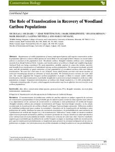
where N is the number of states included in each sum over i and j. For the hydrated electron, the center of mass of the ground state and the lowest three excited states are nearly coincident, as discussed in Section IV, so we have taken rQM to be the center–of–mass position of the hydrated electron’s ground state.37 Using this definition, we have calculated g¯N A from two statistically–independent 5–ps equilibrium adiabatic runs with the electron confined to its quasi–spherical ground state, using i, j = 1, 2, . . . 5, i 6= j. Figure 1 displays the averaged weighted distribution function, g¯N A (r), Eq. 12, for the hydrated electron. The hydrated electron repels the water molecules, so there is no coupling at small separations. The coupling turns on abruptly at ∼1.5 ˚ A, rises to a maximum at ∼3 ˚ A, and falls off roughly exponentially with a decay length of ∼2.7 ˚ A. One could therefore estimate the length scale of the nonadiabatic coupling simply as w ' 1.5 + 2.7 = 4.2 ˚ A. Similarly, the distance between the turn–on at ∼1.5 ˚ A and the point at which the function has fallen to half of its maximum value is ∼3.8 ˚ A. If we instead think of g¯N A (r) as a distribution function, we find that twice the root–mean–squared deviation of r, is ∼4.5 ˚ A. Whichever of the methods we choose suggests that the appropriate value for w is ∼4 ˚ A. In the Appendix, we explore how the nonadiabatic relaxation of the hydrated electron calculated with MF–SD varies with w and we show that small changes in w make little difference in the dynamics: Choosing w anywhere in the range 2–5 ˚ A gives essentially the same results, but significantly larger or smaller values of w lead to very different relaxation dynamics.

III.

NUMERICAL METHODS

In all of the calculations presented here, we performed microcanonical molecular dynamics simulations of a single excess electron in a cubic box 18.17 ˚ A on a side containing 200 classical, flexible water molecules. The water molecules interacted according to the 12

SPC–flex potential,38 and the electron interacted with each water molecule through the pseudopotential of Schnitker and Rossky.39 Although there are other choices,40 we chose this pseudopotential to facilitate comparison with the large body of literature on nonadiabatic hydrated–electron relaxation that uses this potential.5–7,17,18,20,21 All of the interactions were computed using minimum–image periodic boundary conditions41 and were tapered smoothly to zero at half the box length.42 The positions and velocities of the classical water molecules were propagated using the velocity Verlet algorithm,41 with a time step δt = 0.5 fs. The average temperature was ∼300 K at the beginning of the runs and ∼315 K after the excited electron had fully relaxed and reequilibrated, with root–mean–squared deviations of ∼9 K. At each time step of the simulation, the lowest four adiabatic eigenvectors, |φn i (n = 1, 2, 3, 4), were computed at the vertices of a 16 × 16 × 16 cubic lattice with an iterative– and–block Lanczos algorithm.24 The nonadiabatic coupling at time t + δt was computed using a finite–difference approximation, hφi (t)|φj (t + δt)i − hφi (t + δt)|φj (t)i hφi (t + δt)|φ˙ j (t + δt)i = , 2δt

(13)

The nonadiabatic coupling vectors needed for most of the algorithms were calculated using the relation,2 hφl |∇n φk i =

hφl |∇n Vˆ |φk i . k − l

(14)

Once the adiabatic eigenstates and nonadiabatic couplings at time t+δt were calculated, the density matrix was propagated from time t to t+δt in 500 intermediate steps, with each step propagated by a fourth–order Runge–Kutta algorithm; during the Runge–Kutta integration, the adiabatic energies and nonadiabatic couplings were linearly interpolated between their values at time t and their values at time t + δt. For the simulations using the MF–SD algorithm, all of the averages reported in this paper were taken from 50 nonequilibrium trajectories in which the electron was excited at time t = 0 by 2.27 ± 0.01 eV to either the first or second excited state. The 50 runs began with 25 initial water configurations and velocities taken from a 10–ps ground state equilibrium simulation; half of the runs used the initial velocities from the equilibrium simulation and the remaining half used the same initial configurations but with the velocities reversed. For the simulations using the MFSH, FSSH, and EDSH algorithms, the averages were taken from the same 25 initial conditions whose velocities were not reversed. The random numbers 13

used to determine whether a surface hop or wave function collapse occurred in all of these algorithms were generated using the ran2 routine from Numerical Recipes. For the MFSH simulations, the parameters needed to determine when mean–field rescalings take place are the same as those used by Wong and Rossky in Ref. 6. The SPSH results reported in this paper were taken from the 20 excited–state runs reported in Ref. 17.

IV.

EXCITED–STATE RELAXATION OF THE HYDRATED ELECTRON WITH DIFFERENT MQC ALGORITHMS

The hydrated electron is a solvent–supported species with an optical absorption spectrum in the visible and near infrared.43 The most common view is that the hydrated electron is trapped in a roughly spherical cavity with the water polarized around it.39,40,44–48 The low–lying adiabatic eigenstates of the hydrated electron resemble those of a particle in an attractive spherical box: The ground state is approximately s–like and centered in the cavity, and there are three p–like bound states also centered in the cavity, with higher–lying continuum states delocalized in the liquid. Previous nonadiabatic studies of the excited– state relaxation of the hydrated electron using the SPSH algorithm17 have revealed that when the spherically–symmetric electron is excited into a p–like excited state, the energy of the excited state does not change on average throughout the relaxation process. The ground state, in contrast, is rapidly destabilized as water molecules in the first solvation shell move so as to bring hydrogen atoms into the node of the excited orbital. The energy of the ground state continues to rise as the first solvent shell rearranges to accomodate the two lobes of charge until, after a few hundred fs, the ground state energy reaches a quasi–equilibrium several tenths of an eV below the occupied excited–state energy.17 Prior to the establishment of this quasi–equilibrated excited state there are very few surface hops, and even after the system reaches quasi equilibrium, it must wait several hundred fs for an opportunity to hop to the ground state. Thus, with SPSH, the electron collapses to the ground state on average ∼730 fs after the initial excitation. Using a new quantum mechanical projection formalism, we recently have shown that the physical picture of the ground state being destabilized by solvent librations holds when the relaxation dynamics is computed with MF–SD.49 In this Section, we will explore how this picture changes when the dynamics is computed with each of the nonadiabatic MQC algorithms described in Section II. 14

A.

Population dynamics and excited–state lifetimes

Figure 2 displays dynamical histories of the adiabatic and mean–field energies for a representative single hydrated electron relaxation run as calculated using the FSSH (panel A), MFSH (panel B), EDSH (panel C) and MF–SD (panel D) algorithms; each run began with the same initial conditions and random number seed. For the first ∼250 fs, the dynamics computed via all four simulation methods appear identical, characterized primarily by ground–state destabilization, as discussed above, after which small deviations begin to appear. When the dynamics for this trajectory are computed with FSSH, the hydrated electron makes a transition to the ground state at time t = 362.5 fs, and thereafter its trajectory is distinct from the other three nonadiabatic MQC methods. With MFSH dynamics there is little mixing (less than 1%) of multiple adiabatic states and the hydrated electron remains largely in the excited state until the time of the nonadiabatic transition at t = 452.5 fs. With EDSH dynamics, there is minimal mixing in the excited state and the transition to the ground state occurs at the same time as with FSSH dynamics (at the onset of strong mixing of the ground state into the mean–field wave function). After the hop to the ground state, the EDSH mean–field wave function continually re–mixes amplitude with the first excited state until as much as 90% of the wave function consists of the first excited state; in the presence of this much mixing, the system undergoes a surface hop to the first excited state (not shown) followed within 50 fs by a hop back to the ground state. We note that the particular ordering of the relaxation lifetimes seen for the trajectories in Fig. 2 is not unique: For other initial conditions, the electron reaches the ground state first with EDSH or with MFSH dynamics, or all three FSSH–based methods perform a surface hop at almost the same time. Thus, no matter how wave–function mixing is described, the fewest–switches criterion for surface hops causes the transition to occur immediately after the onset of significant nonadiabatic coupling between the ground and first excited state; the subsequent return to equilibrium then thwarts any additional mixing (except for EDSH). In contrast, there is significant mixing of several basis states into the mean–field wave function of the electron with MF–SD dynamics, because unlike the FSSH–based methods, the transition of the system to the ground state is not necessarily induced at the onset of rapid mixing. Furthermore, in MF–SD there is a good chance that a strongly mixed state can collapse back to the excited state, a possibility not allowed by FSSH and seldom achieved

15

with MFSH because strong mixing does not occur without inducing a surface hop. In the MF–SD trajectory for the electron shown in Fig. 2, the mixed MF wave function did in fact collapse back onto the first excited state, at both t = 361 fs and t = 450 fs. The first collapse to the ground state takes place at time t = 931.5 fs, only after the mean–field wave function has built up nearly 50% population on the ground state. Figure 3 displays the averaged excited–state survival probabilities, ps (t) =

X

Θ(tα − t)/N,

(15)

α

computed with SPSH (dotted curve) and MFSH (dashed curve) dynamics, where Θ(t) is a step function, tα is the time of the first transition to the ground state, and N is the number of runs. The averaged EDSH and FSSH results are not shown because they are essentially identical to those produced with MFSH. In MF–SD, the population evolves continuously, so in any given run there is no clear–cut excited–state survival probability. Because MF– SD does not assume the existence of a well–defined reference state, as is done in surface hopping methods, one cannot say that the hydrated electron occupies a single state except immediately following collapses. For example, if the wave function has acquired 70% ground state character before any collapse the electron should neither be considered fully excited nor should it be considered fully relaxed. One way an average excited–state population can be determined, however, is by defining the average fractional excited–state population, Pexc (t) = 1 − ρ¯11 (t) ,

(16)

where the overbar represents an average over all nonequilibrium runs.50 This fractional excited–state population is precisely analagous to the excited–state survival probability for systems with a reference state, ps (t), and Pexc (t) computed with MF–SD also is displayed in Figure 3 (solid curve). The excited–state survival probability falls off fastest with MFSH dynamics and slowest with SPSH dynamics; the mean excited–state population calculated with MF–SD dynamics lies somewhere in between the other two curves. Note also that the greater mixing allowed in MF–SD (cf. Fig. 5B, below) is manifest in the fact that Pexc (t) decays smoothly and continuously instead of in discrete jumps at surface hopping events, as ps (t) does for FSSH, MFSH, EDSH, and SPSH. Figures 2 and 3 make it evident that the extra mixing allowed by MF–SD can alter the dynamics in individual trajectories and thus the average excited–state lifetime for the 16

electron. For methods based on surface hopping, the lifetime of a single run is defined as the time at which the reference state switches to the ground state.17 Thus, the average P lifetime for N excited state runs would be t¯ = α tα /N , where tα is the lifetime for run number α. With EDSH, we take tα to be the time of first transition to the ground state, although the fact that Ehrenfest dynamics allows the continuous build–up of amplitude in the excited state means that the excited–state lifetime of hydrated electrons probably should be considered to be infinite. In MF–SD, because the population evolves continuously there is no clear–cut excited–state lifetime in any given run, but a lifetime can be defined by analogy to the lifetime computed with a reference state. It is straightforward to show that the average lifetime for systems with a reference state can be calculated from ps (t), R∞ dt t (dps (t)/dt) t¯ = R0 ∞ . dt (dp (t)/dt) s 0

(17)

For the case of continuous population transfer, each decrease in Pexc may be thought of as the loss of a single member of a large ensemble, so we define the MF–SD mean lifetime by analogy to Eq. 17, R∞ dt t (dPexc (t)/dt) hti = R0 ∞ . dt (dPexc (t)/dt) 0

(18)

Although taking the derivative of a function contaminated by simulation noise is numerically unstable, a simple integration by parts converts Eq. 18 to the easily evaluable, Z ∞ hti = dt Pexc (t) ,

(19)

0

where we have used the facts that Pexc (0)=1 and Pexc (∞)=0. The averaged squared lifetime may be defined analagously, with the final result that Z ∞ 2 ht i = 2 dt t Pexc (t) .

(20)

0

We will use Eq. 20 to calculate the statistical uncertainty in the mean MF–SD lifetime from p the standard deviation, (ht2 i − hti2 )/(N − 1). Table I displays the average excited–state lifetime for the hydrated electron computed using Eqs. 17 or 18 for the five different nonadiabatic MQC methods. The table makes it clear that the hydrated electron lifetime, t¯, is essentially the same for MFSH, FSSH, and EDSH (although as discussed above EDSH should properly be considered to give an infinite lifetime). Thus, if surface hops take place according the the fewest–switches criterion, 17

it makes no difference in the average lifetime whether the wave function is propagated with complete decoherence (FSSH), complete coherence (EDSH), or something in between (MFSH). This result suggests that changes in the excited–state lifetime must come from changes in the evolution of the density matrix used to determine hopping probabilities. In fact, Tully suggested that decoherence could be incorporated into FSSH by continuously damping the off–diagonal elements of the density matrix,3 and such damping terms have been included by Wong and Rossky in two variants of MFSH,6,7 but is not clear precisely how the damping affects the average excited–state lifetime of hydrated electrons.51 Similarly, we anticipate that the modifications of FSSH introduced by Truhlar and coworkers,10–12 which use fewest–switches probabilites to compute surface hops, but which continuously damp the density matrix elements to complete the hop, will give essentially the same lifetime for the hydrated electron. All three FSSH–based methods discussed in this work result in a much shorter excited–state lifetime than MF–SD. SPSH, which allows coherent propagation between time steps but forces the wave function to collapse after each classical time step, yields a longer lifetime than MF–SD,17 but we do not believe the difference is statistically significant. In the above discussion, we compared hti, Eq. 18, from MF–SD to t¯, Eq. 17, for the other methods because we believe hti provides the closest analog to t¯. But hti is not the only possible definition one could use to define the lifetime with MF–SD dynamics. Although MF–SD does not incorporate the idea of a reference state, one could calculate a version of t¯ in MF–SD by taking the relaxation time for a run to be the time at which the wave function first collapses to the ground state. We would expect this to overestimate the lifetime because it does not include reductions in excited–state character caused by significant mixing into the ground state that can occur before the transition.52 For MF–SD with w = 4.0 ˚ A, calculating t¯ in this fashion gives t¯ = 660 ± 116 fs, where the error is two standard deviations. As expected, this lifetime exceeds the lifetime calculated with hti, Eq. 18 (Table I).

B.

Nonequilibrium solvation response function

The nonequilibrium solvation response for the hydrated electron typically is studied by examining how the energy gap between the occupied and ground states, U (t) = M F (t)−0 (t) evolves after the electron is excited. In principle, U (t) is simply related to the fluorescence 18

Stokes shift,20 but it is often more convenient to examine the normalized nonequilibrium solvent response function, U¯ (t) − U¯ (∞) S(t) = ¯ , U (0) − U¯ (∞)

(21)

where the overbar indicates a nonequilibrium average over the ensemble of excited–state runs. When we compute this nonequilibrium average, we remove runs from the ensemble at the instant the wave function first collapses onto the ground state. Figure 4 displays the nonequilibrium solvation response functions for the excited hydrated electron calculated with FSSH, EDSH, and MF–SD; the MFSH result is not shown for clarity because it is nearly identical to the FSSH and EDSH results. Clearly, there is essentially no difference in the energy relaxation predicted by the different methods, except perhaps for SPSH (not shown).53 We find it surprising that MF–SD gives the same solvent response function as the various fewest–switches based algorithms, because the excited–state lifetime is significantly longer with MF–SD than with these other methods and because we expected the extra mixing with MF–SD to lower the gap relative to the other algorithms. We believe that the explanation for this is that S(t) is ill–suited to detect differences in the excited– state dynamics for this system. As discussed above, Schwartz and Rossky have shown17 (and we have confirmed49 ) that most of the dynamics inherent in the electron’s S(t) comes from destabilization of the ground state as the solvent rearranges around the excited electron. The extra mixing allowed with MF–SD only affects the energy gap near the transition to the ground state, and this has little effect on the shape of S(t) because most of the dynamics come from the large shift in the ground–state energy. Apparently, solvent migration into the node of the excited electron is unaffected by whether or not there is a few percent of another state mixed into the wave function, so the ground–state destabilization that dominates S(t) is insensitive to the differences in population dynamics.

V.

DISCUSSION: THE EFFECTS OF DECOHERENCE ON CONDENSED–PHASE NONADIABATIC DYNAMICS

In this paper, we have compared the excited–state relaxation dynamics of the hydrated electron calculated by five different nonadiabatic MQC algorithms. Most of the algorithms use the idea of a “reference state,” with a rule for switching the reference state in what is 19

called a surface hop. Three of the methods, FSSH, MFSH, and EDSH, are based on Tully’s fewest–switches method for computing the probability of a surface hop; in our interpretation, they represent, respectively, the rapid, intermediate, and minimal decoherence regimes. The hopping criterion in SPSH resembles the fewest–switches prescription in the limit of small time step, whereas MF–SD uses a fundamentally different decoherence criterion. We have found, however, that with fewest–switches hops, the amount of decoherence has no effect on the excited–state lifetime of the hydrated electron. Instead, the lifetime appears to be controlled entirely by the fewest–switches criterion, suggesting that FSSH (and its siblings MFSH and EDSH) do not properly include the effects of decoherence for the hydrated electron. This suggests that for FSSH, decoherence should be included either through a sum of amplitudes over a swarm of trajectories or by damping of elements of the density matrix.3,6,7 The similarity of the FSSH and MFSH results also suggests that MFSH is merely a more expensive way to do FSSH; this is consistent with the fact that MFSH and FSSH gave the same answers for the one–dimensional single avoided crossing problem,1,2 which has similar physics to the hydrated electron’s relaxation. Our results for EDSH relaxation also showed an interesting difference from what would be expected with purely Ehrenfest dynamics. Parandekar and Tully have shown that true Ehrenfest dynamics leads to equal population of all states,29 and we have confirmed this for the hydrated electron.54 The presence of surface hops, however, seems to bias the system towards the occupying either the ground or first excited state, and we speculate that EDSH may yield average populations intermediate between the infinite–temperature (Ehrenfest dynamics) and properly Boltzmann weighted (FSSH dynamics)55 limits. Despite the differences in excited–state dynamics and lifetimes with the different nonadiabatic MQC algorithms, we found that all of the methods we tested produced identical nonequilibrium solvation response functions, S(t). This is because the dynamics underlying S(t) for the hydrated electron are dominated by solvent motions that depend only weakly on details of the excited–state wave function. In addition to FSSH–based algorithms, we also applied the MF–SD algorithm to the relaxation of the hydrated electron, the first time MF–SD has been applied to a condensed– phase problem. As far as we are aware, MF–SD is the only MQC algorithm that considers all nonadiabatic transitions to be induced by decoherence instead of imposing a separate transition criterion based on the time evolution of the quantum wave function. The deco20

herence time scale is set by the effective width of Gaussians that are imagined to model quantum aspects of the classical degrees of freedom, and we described in detail how one goes about finding the Gaussian width parameter that determines decoherence in MF–SD. In the Appendix, we show that small changes in the width parameter, w, have little effect on the overall relaxation dynamics, but that large changes lead to drastically different excited–state lifetimes. In either the rapid or slow decoherence limit, the lifetime of the excited state diverges, in the former case because of the quantum Zeno effect,56 and in the latter case because Ehrenfest dynamics never leads to a fully–populated ground state.29 For decoherence in the intermediate regime, w ∼ 2–5, we find that the lifetime does not change appreciably, so one only needs to estimate w to apply MF–SD to a condensed–phase problem. In the Appendix, we also point out that the range for w that we believe to be correct produces the smallest excited–state lifetimes, and we speculate that this minimum is not coincidental: Identifying such a minimum could provide an (albeit expensive) alternative method for determining w. When we originally introduced MF–SD, we showed that for three standard, one– dimensional model problems MF–SD is at least as accurate as methods based on fewest– switches surface hopping, and that for some problems it is much more accurate.1 Having now applied this method to hydrated–electron relaxation, a problem whose exact solution is not known, we find that MF–SD dynamics differs in several important ways from FSSH and its siblings. First, in MF–SD the wave function of the system is allowed to mix much more than in FSSH or MFSH. Near a transition to the ground state, MF–SD yields an electronic structure that is a superposition of the ground and excited states for tens of fs. Fewest–switches–based algorithms, in constrast, hop to the ground state as soon as mixing begins to occur, so that far less mixing actually takes place near the transition. Second, the criteria used to decide when to collapse the wave function are very different for the two methods. With fewest–switches, strong mixing causes a surface hop, whereas in MF–SD a wave function collapse only occurs if the mixing would lead to a loss of overlap among the Gaussians that represent the classical particles. We already have shown that this difference allows MF–SD dynamics to correctly predict reflection and transmission probabilities without spurious St¨ uckelberg oscillations for Tully’s extended–coupling model,1,3 and we saw here that this difference also leads the hydrated electron to maintain excited–state character on average ∼200 fs longer for MF–SD than for FSSH or MFSH. 21

Because the calculated S(t) for the hydrated electron is similar for all methods, each would produce dynamics that compare equally well to experiment. Thus, the question is which nonadiabatic MQC algorithm incorporates the most intuitively correct physics. Our preference is for MF–SD for two main reasons. First, MF–SD allows the time–dependent Schr¨odinger equation to govern evolution of the wave function until decoherence induces changes in the dynamics. Second, MF–SD allows mixed states to exist so long as the classical particles cannot distinguish mixed from unmixed states, so that collapses of the wave function are induced by the classical particles “making a measurement” on the quantum sub–system and not by the rate of change of the quantum system’s density matrix (which in our view should have little to do with whether the classical bath will attempt to collapse the wave function). As a consequence, wave function collapses need not occur at the onset of rapid mixing, and our intuition suggests that this may provide a more correct description of the quantum dynamics for systems with weak nonadiabatic coupling between the ground and excited states, such as the hydrated electron. We believe that there is room for considerably more discussion of exactly how it is that decoherence controls excited–state relaxation in the condensed phase, particularly because we cannot rely on experiments on hydrated electron relaxation to decide among the nonadiabatic MQC algorithms. We hope that the detailed examination given here has clarified some of the issues involved in choosing a nonadiabatic MQC algorithm, and that these questions, whose answers we have only been able to hint at, will provide the impetus for further research into how decoherence should properly be included in MQC dynamics.

Acknowledgments

Funding for this research was provided by NSF grant No. CHE-0204776. B.J.S is a Camille Dreyfus Teacher–Scholar. We gratefully acknowledge the use of the California Nano Systems Institute Beowulf cluster for many of the calculations described in this paper.

22

APPENDIX: w–DEPENDENCE OF THE EXCITED–STATE LIFETIME OF THE HYDRATED ELECTRON

In the one–dimensional problems for which we previously tested MF–SD, we found that small changes in the width parameter, w (defined in Eq. 10), made little difference in the MQC dynamics.1 Changing w by a factor of two or more did, however, cause significant differences in the nonadiabatic transition probabilities. In this Appendix, we examine the dynamics of excited hydrated electrons calculated with MF–SD as a function of w, and we discuss in detail what changing w implies for the resulting dynamics. Each of the average lifetimes reported here for the 15 different choices of w represents between 75 and 250 dedicated hours on a single AMD Opteron 248 processor; we were able to perform the calculations in days rather than months through the use of many such processors on a large Beowulf cluster. Figure 5 shows, for the same initial condition, the populations, ρii , as a function of time after resonant excitation of a hydrated electron by 2.26 eV to the first excited state for several different choices of w. Panel A shows that setting w = 0.1 ˚ A, much smaller than the 4 ˚ A suggested by the discussion in Section II D, causes the wave function to collapse at nearly every time step (on average, after 99.7% of the timesteps). Such frequent collapses are expected because a small value of w implies a large decoherence rate, τ −1 . Over the short time between collapses, very little mixing with the ground state can occur, so by Eq. 8 there is almost no chance for the electronic wave function to collapse to the ground state; the collapse to the ground state t=767 fs occured only after a chance reduction in the energy difference between the ground and first excited states allowed significant mixing into the ground state in a single 0.5–fs time step. Panel B displays the evolution of the populations with our presumptive choice of w = 4 ˚ A. This Gaussian width allows significantly more mixing to take place, so that there are only three wave function collapses over the entire run, as indicated by the crosses in panel B. As the inset shows, ∼350 fs after the initial excitation, population builds up on the ground state, reaching a plateau with ∼70% population on the ground state and only ∼30% on the first excited state. After only ∼15 fs as a strongly–mixed state, decoherence induces a wave function collapse to the ground state. After the ground state has been reached, solvation quickly reduces the ground–state energy so there is very little further mixing. Finally, panel C shows the population dynamics with w = 10 ˚ A. The 23

large w implies very broad Gaussians in momentum space, so there should be very few wave function collapses. As indicated by the crosses in panel C, over the 1.6 ps of this simulation, there were only two decoherence events, one that caused a collapse back to the first excited state at ∼680 fs and the other that caused a collapse to the ground state at ∼1370 fs. The lack of decoherence events over a relatively long time means that the calculated dynamics is very nearly Ehrenfest in character, with the wave function remaining mixed for excessively long periods. It recently has been shown that such mean–field dynamics leads on average to equal populations in all states,29 so that as w → ∞ the electron will never be confined solely to a single state; in this limit, MF–SD should approach purely Ehrenfest dynamics. Figure 5 showed that either with very large or very small values of w, the electron remains in the excited state for significantly longer than we saw with the intermediate value, w = 4 ˚ A. Thus, in Fig. 6 we study the w–dependence of the average excited–state lifetime of the hydrated electron. The upper panel of Figure 6A shows the average excited state population, Pexc (t) (Eq. 16), for the same three width parameters discussed in connection with Figure 5. The solid curve shows that on average Pexc (t) decays fastest for w = 4 ˚ A. The dashed curve, for w = 10 ˚ A, decays more slowly but varies continuously, as expected for what is largely mean–field dynamics with only a few wave function collapses. The dotted curve, for w = 0.1 ˚ A, differs markedly from the other two average excited–state populations. The population decreases in a stepwise fashion because the density matrix is constantly being collapsed to one of the excited states, as in the quantum Zeno effect.56 In this rapid decoherence limit, the steps in Pexc (t) correspond to the times when the essentially adiabatic dynamics of an excited state switches to become adiabatic dynamics on the ground electronic state. Thus, Pexc (t) for w = 0.1 ˚ A is closely analagous to the excited–state survival probability calculated in other surface hopping techniques,2,3 albeit with a different (and quite artificial) criterion for the hops. We have seen that different values of w lead to distinct dynamics for the density matrix. How do these differences translate into a lifetime for the excited hydrated electron? Figure 6B displays the mean lifetime as a function of w for Gaussian widths ranging from 0.1 ˚ A up to 20 ˚ A, where each point is calculated using Pexc (t) averaged over 50 excited–state relaxation runs as described in Section III. As expected from our earlier discussion, at both small and large w, the lifetime is quite large. In the limits w → 0 and w → ∞, the lifetime rigorously becomes infinite, consistent with the trends shown in the figure; for w ≥ 5 ˚ A, 24

the lifetime fits very well to an exponential increase with w. The mean lifetime does not change significantly for 2 ≤ w ≤ 5, so any of the methods we used to estimate w can be considered equivalent. The fact that the mean lifetime in this range of w is a minimum raises the intriguing possibility that the correct value of w may be found by looking for the minimum lifetime, especially because a minimum lifetime represents a balance between allowing mixing to occur (unlike with w ∼ 0) and not allowing decoherence events (as with w → ∞). It is interesting to speculate that it may not be a coincidence that the minimum lifetime occurs with the value of w determined by examining Eq. 12, but as of yet we have no compelling argument for why this should be the case.

1

Bedard-Hearn, M. J.; Larsen, R. E.; Schwartz, B. J. J. Chem. Phys. 2005, 123, 234106.

2

Prezhdo, O. V.; Rossky, P. J. J. Chem. Phys. 1997, 107(3), 825–834.

3

Tully, J. C. J. Chem. Phys. 1990, 93(2), 1061–1071.

4

Webster, F.; Wang, E. T.; Rossky, P. J.; Friesner, R. A. J. Chem. Phys. 1994, 100(7), 4835– 4847.

5

Wong, K. F.; Rossky, P. J. J. Phys. Chem. A 2001, 105(12), 2546–2556.

6

Wong, K. F.; Rossky, P. J. J. Chem. Phys. 2002, 116(19), 8418–8428.

7

Wong, K. F.; Rossky, P. J. J. Chem. Phys. 2002, 116(19), 8429–8438.

8

Berne, B. J., Ciccoti, G., Coker, D. F., Eds. Classical and Quantum Dynamics in Condensed Phase Simulations: Proceedings of the International School of Physics “Computer simulation of rare events and dynamics of classical and quantum condensed–phase systems”; World Scientific, Singapore, 1998.

9

Neria, E.; Nitzan, A.; Barnett, R. N.; Landman, U. Phys. Rev. 1991, 67(8), 1011–1014.

10

Hack, M. D.; Truhlar, D. G. J. Chem. Phys. 2001, 114, 9305.

11

Zhu, C. Y.; Jasper, A. W.; Truhlar, D. G. J. Chem. Phys. 2004, 120, 5543.

12

Zhu, C. Y.; Nangia, S.; Jasper, A. W.; Truhlar, D. G. J. Chem. Phys. 2004, 121, 7658.

13

Hammes-Schiffer, S.; Tully, J. C. J. Chem. Phys. 1994, 101(6), 4657–4667.

14

Martinez, T. J.; Ben-Nun, M.; Levine, R. D. J. Phys. Chem. 1996, 100, 7884.

15

Ben-Nun, M.; Martinez, T. J. J. Chem. Phys. 2000, 112, 6113.

16

Drukker, K. J. Comput. Phys. 1999, 153, 225.

25

17

Schwartz, B. J.; Rossky, P. J. J. Chem. Phys. 1994, 101(8), 6902–6916.

18

Schwartz, B. J.; Rossky, P. J. J. Chem. Phys. 1994, 101(8), 6917–6926.

19

Murphrey, T. H.; Rossky, P. J. J. Chem. Phys. 1993, 99(1), 515–522.

20

Schwartz, B. J.; Rossky, P. J. J. Phys. Chem. 1995, 99, 2953.

21

Schwartz, B. J.; Rossky, P. J. J. Chem. Phys. 1996, 105(16), 6997–7010.

22

Schwartz, B. J.; Bittner, E. R.; Prezhdo, O. V.; Rossky, P. J. J. Chem. Phys. 1996, 104, 5942.

23

Bittner, E. R.; Schwartz, B. J.; Rossky, P. J. J. Mol. Struct. (Theochem) 1997, 389, 203.

24

Webster, F.; Rossky, P. J.; Friesner, R. A. Comp. Phys. Comm. 1991, 63(1-3), 494–522.

25

For the evolution in terms of a general basis set, see Ref. 1.

26

Pechukas, P. Phys. Rev. 1969, 181, 166.

27

Pechukas, P. Phys. Rev. 1969, 181, 174.

28

McWhirter, J. L. J. Chem. Phys. 1999, 110(9), 4184.

29

Parandekar, P.; Tully, J. C. J. Chem. Theory Comput. 2006, 2, 229.

30

Schrodinger, E. Proc. Am. Philos. Soc. 1980, 124, 323.

31

Zurek, W. H. Phys. Today 1991, 44(10), 36.

32

Tully, J. C.; Preston, R. K. J. Chem. Phys. 1971, 55, 562.

33

To our knowledge, the EDSH algorithm presented here has never before been used. As noted in the text, for us EDSH represents only the minimal–decoherence limit of the MFSH algorithm (Ref. 2).

34

M¨ uller, U.; Stock, G. J. Chem. Phys. 1997, 107, 6230.

35

An alternate method for computing characteristic decoherence times has been suggested by Jasper, A.W.; Truhlar, D.G., J. Chem. Phys. 2005, 123, 064103.

36

Prezhdo, O. V.; Rossky, P. J. J. Phys. Chem. 1996, 100, 17094.

37

In a system where the different adiabatic eigenstates may be spatially separated, as for an excess electron in tetrahydrofuran (see Ref. 57), rQM would need to be defined appropriately, e.g. rQM = ri , where ri = hφi |r|φi i for each adiabatic state i.

38

Toukan, K.; Rahman, A. Phys. Rev. B 1985, 31(5), 2643–2648.

39

Schnitker, J.; Rossky, P. J. J. Chem. Phys. 1987, 86(6), 3462–3470.

40

Turi, L.; Borgis, D. J. Chem. Phys. 2002, 117(13), 6186–6195.

41

Allen, M. P.; Tildesley, D. J. Computer Simulation of Liquids; Oxford University Press, London, 1992.

26

42

Steinhauser, O. Mol. Phys. 1982, 45, 335.

43

Jou, F.-Y.; Freeman, G. R. J. Phys. Chem. 1979, 83, 2383.

44

Schnitker, J.; Motakabbir, K.; Rossky, P. J.; Friesner, R. Phys. Rev. 1988, 60(5), 456–459.

45

Kevan, L. Acc. Chem. Res. 1981, 14(5), 138–145.

46

Staib, A.; Borgis, D. J. Chem. Phys. 1995, 103(7), 2642–2655.

47

Tauber, M. J.; Mathies, R. A. J. Am. Chem. Soc. 2003, 125(5), 1394–1402.

48

Larsen, R. E.; Schwartz, B. J. J. Phys. Chem. B 2006, 110, 1006.

49

Bedard-Hearn, M. J.; Larsen, R. E.; Schwartz, B. J. Submitted to Phys. Rev. Lett.

50

In the nonequilibrium average for Eq. 16, all 50 excited–state runs are included at all times. Runs that reached the ground state and re¨equilibrated soonest were not propagated as long as other runs, however, so for times after these runs terminated, we take 1 − ρ11 (t) to be zero in the averaging.

51

Wong and Rossky (WR) have reported significant lifetime differences for the excited hydrated electron as the damping of off–diagonal density matrix elements in MFSH is changed (Ref. 6), but we believe that this result is an artifact of an incorrect statistical procedure. To compute the mean lifetime with different damping parameters, WR used a small number of trajectories for each value of the damping parameter but resampled transition probabilities for each trajectory using hundreds of different random number seeds. Unfortunately, this resampling procedure cannot produce correct average lifetimes because for the hydrated electron, the ground–to–first– excited–state energy gap opens rapidly after the transition to the ground state; the resampling therefore severely underestimates the probability of surface hops for times later than the surface hop for the original run. Thus, average lifetimes computed with this resampling procedure will be artificially long.

52

For example, in simulations of the excited–state relaxation of electrons solvated in liquid tetrahydrofuran (Ref. 58) the electron often populates the ground state entirely by continuously mixing more and more ground–state character into the mean–field wave function, with no discontinuous collapse to the ground state ever taking place.

53

The nonequilibrium solvent response function, S(t), predicted with SPSH in Ref. 17 has a smaller inertial decay than is seen in any of the curves in Fig. 4. At the early “bounce,” the SPSH S(t) is only ∼0.6 rather than ∼0.4 as seen in Fig. 4. This difference may be caused by dynamics with SPSH that is distinct from that predicted with any of the other MQC algorithms

27

discussed in this paper, but we cannot say this for certain. The difference also may be a result of poor sampling of initial conditions. 54

Larsen, R. E.; Schwartz, B. J. unpublished.

55

Parandekar, P.; Tully, J. C. J. Chem. Phys. 2005, 122, 094102.

56

Chiu, C. B.; Sudarshan, E. C. G.; Misra, B. Phys. Rev. D 1977, 16, 520.

57

Bedard-Hearn, M. J.; Larsen, R. E.; Schwartz, B. J. J. Chem. Phys. 2005, 122, 134506.

58

Bedard, M. J. Understanding classical and quantum solvation dynamics in the weakly polar solvent tetrahydrofuran (THF) using projections of molecular motions in molecular dynamics simulations PhD thesis, University of California, Los Angeles, 2006.

28

MQC algorithm Lifetime (fs)a

a The

MF–SDb

632 ± 116

SPSHc

731 ± 217

MFSHd

445 ± 111

FSSHe

409 ± 112

EDSHf

532 ± 144†

lifetimes were calculated using Eq. 19 for MF–SD and using Eq. 17 for the other methods;

the integrations were performed using the trapezoid rule with a time step of 0.5 fs. b Mean–field

dynamics with stochastic decoherence (Ref. 1 and this work), computed with the

Gaussian width parameter w = 4.0 ˚ A and 50 runs, as described in the text. c Stationary–phase

with surface hopping (Refs. 4 and 24), taken from the 20 runs reported in

Ref. 17. d Mean–field

dynamics with surface hopping (Refs. 2 and 5) with 25 runs.

e Fewest–switches

surface hopping (Ref. 3) with 25 runs. As described in the text, these runs used

a single trajectory for each initial condition rather than the swarm of trajectories required by the original formulation of the method. f Ehrenfest †

dynamics with surface hopping (this work) with 25 runs.

As discussed in the text, it may be more appropriate to consider the excited–state lifetime to be

infinite with EDSH dynamics.

TABLE I: Average excited–state lifetime of the hydrated electron computed via different nonadiabatic MQC algorithms. The uncertainties are two standard deviations, where one standard deviation is calculated as described in the text from the root–mean–squared deviation divided by √ N − 1, where N is the number of runs.

29

FIG. 1: Nonadiabatic–coupling–weighted radial distribution function, Eq. 12, for the hydrated electron.

FIG. 2: Representative dynamical histories of the excited hydrated electron’s adiabatic (alternating thin solid and dashed gray curves) and mean–field (thick solid curve) energies calculated with FSSH (panel A), MFSH (panel B), EDSH (panel C), and MF–SD (w = 4.0 ˚ A, panel D). The crosses show times at which the mean–field wave function was collapsed onto a single adiabatic state.

FIG. 3: Average excited–state probability of the hydrated electron calculated with with MF–SD (Pexc (t), solid curve, Eq. 16), and excited–state survival probability (ps (t), Eq. 15) with MFSH (dashed curve) and SPSH (dotted curve). FSSH and EDSH excited–state survival probabilities are not shown because they are indistinguishable from the MFSH result.

30

FIG. 4: Nonequilibrium solvation response, Eq. 21, of the excited hydrated electron, computed with MF–SD (solid curve), FSSH (dashed curve) and MFSH (dotted curve); the S(t) computed with EDSH is not shown because it is indistinguishable from the FSSH and MFSH results. The S(t)’s were computed using 25 trajectories started from the same initial conditions for MF–SD as for FSSH and MFSH. FIG. 5: Time evolution of the state populations calculated with MF–SD following excitation of a hydrated electron for different choices of the width parameter w (Eq. 10): w = 0.1 ˚ A (panel A), w = 4.0 ˚ A (panel B), and w = 10.0 ˚ A (panel C). The insets in panels A and B show the times near the first wave function collapse to the ground state on an expanded scale. The crosses in panels B and C indicate times at which the wave function collapsed to a single adiabatic state; wave function collapses are not indicated in panel A because when w = 0.1 ˚ A, the wave function collapses at almost every time step, as discussed in the text.

FIG. 6: Average excited–state population and lifetimes for the hydrated electron calculated with MF–SD for different width parameters w, Eq. 10. Panel A: Average 1 − ρ11 (t) for w = 0.1 ˚ A (dotted curve), w = 4.0 ˚ A (solid curve), and w = 10.0 ˚ A (dashed curve). Panel B: Average MF–SD excited–state lifetime, Eq. 18, of the hydrated electron as a function of w. The error bars are plus or minus two standard deviations. As is discussed in the text, we have estimated the optimum value of the width parameter for this system to be w ' 4 ˚ A.

31

g(r) (arb. units)

1 0.8 0.6 0.4 0.2 0

0 1 2 3 4 5 6 7 8 9 10 r (Å)

Larsen, Bedard-Hearn and Schwartz, JPC, Fig. 1

(A)

FSSH

(B)

MFSH

(C)

EDSH

(D)

MF-SD

Energy (eV)

1 0 -1 -2 -3

Energy (eV)

1 0 -1 -2 -3 0 200 400 600 800 1000 Time (fs)

200 400 600 800 1000 Time (fs)

Larsen, Bedard-Hearn and Schwartz, JPC, Fig. 2

1 MF-SD MFSH SPSH

Pexc(t) , ps(t)

0.8 0.6 0.4 0.2 0

0

500

1000 1500 Time (fs)

2000

Larsen, Bedard-Hearn and Schwartz, JPC, Fig. 3

1 MF-SD FSSH MFSH

0.8 S(t)

0.6 0.4 0.2 0 -0.2

0

200

400 Time (fs)

600

Larsen, Bedard-Hearn and Schwartz, JPC, Fig. 4

1

(A) 0.8

Pop.

Population

1

0.6 0.4

w = 0.1 Å

0.2 0

1

(B)

0.8

Pop.

Population

0 740 760 780 Time (fs)

0.6 0.4

0 340 360 380 Time (fs)

0.2

w=4Å

Population

0

(C)

0.8 0.6 0.4

w = 10 Å

0.2 0

0

400

800 1200 Time (fs)

1600

Larsen, Bedard-Hearn and Schwartz, JPC, Fig. 5

1

(A)

Pexc(t)

0.8

w=4Å w = 10 Å

0.6 0.4

w = 0.1 Å

0.2 0

0

1

2

5

3

4 5 6 Time (ps)

7

8

(B)

〈 t 〉 (ps)

4 3 2 1 0

0

5

10 w (Å)

15

20

Larsen, Bedard-Hearn and Schwartz, JPC, Fig. 6