PHYSICAL REVIEW B 81, 155119 共2010兲

Extension of exact-exchange density functional theory of solids to finite temperatures Maximilian Greiner Lehrstuhl für Theoretische Chemie, Universität Erlangen-Nürnberg, Egerlandstraße 3, D-91058 Erlangen, Germany

Pierre Carrier Department of Computer Science and Engineering, University of Minnesota, 4-192 EE/CS Building, 200 Union Street SE, Minneapolis, Minnesota 55455, USA

Andreas Görling Lehrstuhl für Theoretische Chemie, Universität Erlangen-Nürnberg, Egerlandstraße 3, D-91058 Erlangen, Germany 共Received 8 December 2009; revised manuscript received 24 February 2010; published 22 April 2010兲 A general finite-temperature exact-exchange 共EXX兲 formalism derived within the framework of finitetemperature density functional theory for grand canonical ensembles is presented. Based on this formalism a finite-temperature EXX method for solids using plane-wave basis sets is presented. The method is generally applicable, i.e., applicable to insulators, semiconductors, or metals and enables the investigation of temperature effects. More important, however, is that the finite-temperature EXX method enables an EXX treatment of metals by introducing a physically motivated Fermi broadening technique. We tested the method by applying it to sodium, magnesium, and aluminum and compare EXX and LDA 共local density approximation兲 band structures as well as the density of states for the three metals. Differences between LDA and EXX band structures are negligible up to the Fermi level. Above the Fermi level, however, differences between LDA and EXX band structures of magnitudes of 1–2 eV start to build up for energetically higher bands. The magnitude of these differences is of the same order as that of the increases in EXX band gaps compared to LDA band gaps as they are reported for semiconductors and insulators. DOI: 10.1103/PhysRevB.81.155119

PACS number共s兲: 71.15.Mb, 71.45.Gm, 71.55.Ak

I. INTRODUCTION

A basic shortcoming of conventional density functional methods, i.e., of Kohn-Sham 共KS兲 methods relying on exchange-correlation functionals within the local density approximation 共LDA兲 共Refs. 1–3兲 or generalized gradient approximations 共GGAs兲,1–5 is the presence of unphysical Coulomb self-interactions. The Coulomb energy is defined as the energy of the classical electrostatic interaction of the electron density of an electronic system with itself. The Coulomb energy therefore contains unphysical contributions from the interaction of each electron with itself. Similarly, if the Coulomb potential, the classical electrostatic potential of the electron density, acts on an electron of the system then this electron is subject to an interaction with itself because the electron contributes to the electron density. This unphysical Coulomb self-interaction is cancelled by the exchange energy and potential, respectively. In conventional KS methods, however, the Coulomb energy and potential is calculated exactly while the exchange energy and potential is approximated. As a result the cancellation of unphysical Coulomb self-interactions is incomplete. The presence of unphysical Coulomb self-interactions has severe consequences. Conventional exchange-correlation potentials are not attractive enough and, in finite systems, exhibit the wrong asymptotic behavior.6–11 As consequence, the simplest system, the hydrogen atom, is not treated correctly, the additional electron in small anions often is erroneously unbound.12–14 Moreover, the KS orbital and eigenvalue spectrum of conventional KS methods is qualitatively wrong.1–3,12–15 In finite systems the energetical difference of 1098-0121/2010/81共15兲/155119共12兲

the highest occupied molecular orbital 共HOMO兲 to the lowest unoccupied molecular orbital 共LUMO兲 is too small and no Rydberg series exist in eigenvalue spectra. In periodic solids band structures are affected. Conventional KS band gaps of semiconductors are much lower than experimental ones. In how far this is due to the principle difference between the KS band gap and the true quasiparticle band gap and in how far this is due to Coulomb self-interactions is an open question.16–27 However, conventional KS band structures may even be qualitatively wrong exhibiting metallic instead of semiconductor characteristics, like, e.g., in the case of germanium.28 Exact-exchange 共EXX兲 KS methods28–60 solve this basic problem because they treat exactly the exchange energy and the local multiplicative KS exchange potential. The latter must not be confused with the nonlocal Hartree-Fock exchange potential. Hartree-Fock methods lead to occupied orbitals that are free of Coulomb self-interactions, but to unoccupied orbitals that are not. These unoccupied orbitals have little physical meaning. In EXX methods qualitatively correct orbital and eigenvalue spectra are obtained. In finite systems larger HOMO LUMO gaps emerge and Rydberg series are present. In solids qualitatively correct band structures are obtained.28,35,37,49–51,59,60 In small and medium band gap semiconductors EXX band gaps are close to the experimental ones. Whether this agreement between KS and true quasiparticle band gaps would become worse if also the exact correlation potential could be employed is an open question.16–27 In present EXX methods correlation is either neglected or treated via conventional LDA or GGA functionals. It turns out that the choice for the conventional correla-

155119-1

©2010 The American Physical Society

PHYSICAL REVIEW B 81, 155119 共2010兲

GREINER, CARRIER, AND GÖRLING

tion potential or even its complete neglect has little effect on the KS eigenvalue spectra. KS orbitals and eigenvalues are the starting point for methods like the GW method to calculate quasiparticle band structures51,61–63 or for methods based on time-dependent density functional theory in the response regime to treat optical properties.64,65 KS methods providing qualitatively correct band structures therefore are of importance. EXX methods are such methods. Another advantage of EXX methods is that treating exchange energy and potential exactly represents a step in a systematical improvement of density functional methods. The exchange energy is the largest fraction of the exchangecorrelation energy and in contrast to conventional KS methods no longer needs to be approximated. Conventional KS methods strongly rely on error cancellations between exchange and correlation.1–5 Such error cancellations obviously are no longer present if exchange is treated exactly. However, such error cancellations, in any case, can only be exploited for exchange-correlation energies but not for exchange-correlation potentials. For example, the long-range behavior of the effective KS potential is determined exclusively by the exchange potential which exhibits a long-range 共−1 / r兲-behavior with r denoting the distance from the electronic system. The LDA or GGA correlation potentials like the true correlation potential are short-ranged and also the LDA or GGA exchange potentials are short-ranged. Thus the correct long-range 共−1 / r兲-behavior of the exchange potential can never occur due to error cancellations between conventional exchange and correlation potentials. EXX methods have been introduced for atoms,30 solids28,35–37 as well as molecules.40,41 EXX methods for molecules based on Gaussian basis sets are numerically demanding40,43,45,66–68 and only recently a numerically stable method was introduced.57 EXX methods for solids based on plane-wave basis sets,28,36,37 on the other hand, turn out to be numerically stable provided the plane-wave cutoffs for the representation of the orbitals and of the exchange potential are well balanced. However, so far only EXX methods for the limit of zero temperature have been developed. In this work we present a general finite-temperature EXX formalism within the framework of finite-temperature density functional theory for grand canonical ensembles.69 The basic formalism is valid and applicable for finite as well as infinite systems. In this work we then focus on a finitetemperature EXX method for solids based on plane-wave basis sets and test it by applying it to simple metals. For the treatment of periodic solids we have to consider a fixed electron number in order to guarantee charge neutrality of the system, i.e., we cannot freely choose the chemical potential of the grand canonical ensemble but we have to set the chemical potential to a value leading to the required number of electrons. This means we effectively switch from a grand canonical ensemble to a canonical ensemble. The motivation for this work is twofold. On the one hand, this opens the route to investigate temperature effects within an EXX framework. On the other hand, a finite-temperature approach may be used as technical procedure in the k-point sampling in a KS treatment of metals. In order to avoid the use of prohibitively large numbers of k-points “band broad-

ening” schemes are often used in the KS treatment of metals. In EXX methods the k-point sampling is especially critical because in the construction of the exact exchange potential the KS response function is required which contains terms with differences of occupied and unoccupied KS eigenvalues in the denominator. If KS eigenvalues of a k point at the Fermi level are degenerate this may lead to singularities. By using a “band broadening” scheme that has physical meaning such singularities are avoided. This work is organized as follows. In Sec. II the EXX formalism is generalized to finite temperature by deriving an EXX formalism within the general framework of finitetemperature density functional theory for grand canonical ensembles.69 In Sec. III the implementation and computational details are briefly described. In Sec. IV results of applying the new method to the metals sodium, magnesium, and aluminum are presented. Finally, Sec. V contains concluding remarks. II. FINITE-TEMPERATURE EXX FORMALISM A. Basic formalism and definition of energy functionals

An electronic system at finite temperature that can interchange electrons with its environment is described by the density matrix ⌫ˆ v,T,␮ if treated as grand canonical ensemble. The density matrix ⌫ˆ v,T,␮ among all density matrices ⌫ˆ is the one that minimizes the grand potential ⍀关⌫ˆ 兴 共Ref. 1兲 ˆ + kT ln ⌫ˆ − ␮Nˆ兴 ⍀关⌫ˆ 兴 = Tr ⌫ˆ 关H

共1兲

⍀v,T,␮ = min ⍀关⌫ˆ 兴

共2兲

according to ⌫ˆ

for the Hamiltonian operator ˆ = Tˆ + Vˆ + vˆ , H ee

共3兲

the temperature T, and the chemical potential ␮. In Eq. 共3兲, Tˆ and Vˆee designate the operators of the kinetic energy and the electron-electron interaction energy, respectively, while vˆ denotes the operator corresponding to a local multiplicative external potential v共r兲, usually the potential of the nuclei. In ˆ denotes the number operator and k the Boltzmann Eq. 共1兲, N ˆ 关⌫ˆ 兴 are functionals of the constant. The grand potentials ⍀ ˆ ˆ density matrices ⌫, the minimum ⍀ v,T,␮ of the grand potential given in Eq. 共2兲 corresponds to the minimizing density matrix ⌫ˆ v,T,␮, i.e., ⍀v,T,␮ = ⍀关⌫ˆ v,T,␮兴.

共4兲

The minimizing density matrix ⌫ˆ v,T,␮ is given by exp关共− 1/kT兲共EN,n − ␮N兲兴 ⌫ˆ v,T,␮ = 兺 兺 兩⌿N,n典具⌿N,n兩 Zv,T,␮ N n 共5兲 with the grand partition function

155119-2

PHYSICAL REVIEW B 81, 155119 共2010兲

EXTENSION OF EXACT-EXCHANGE DENSITY…

Zv,T,␮ = 兺 兺 exp关共− 1/kT兲共EN,n − ␮N兲兴.

共6兲

n

N

In Eqs. 共5兲 and 共6兲 ⌿N,n denotes the nth N-electron eigenstate of the Hamiltonian operator 共3兲 and EN,n the corresponding energy eigenvalue. Strictly speaking, it is not correct to speak of one Hamiltonian operator 共3兲 because for each particle number N there is a different Hamiltonian operator. Therefore, a reference to the Hamilton operator 共3兲 shall always imply a reference to the appropriate N-electron Hamilton operators. This also holds true in formulas like those in Eqs. 共1兲 and 共2兲 where traces of Hamiltonian operators with density matrices containing contributions with different particle numbers occur. Following the constrained-search formulation of density functional theory1,70,71 we now rewrite the minimization 共2兲, ˆ + kT ln ⌫ˆ − ␮N ˆ 兴其‰ ⍀v,T,␮ = minˆmin兵Tr ⌫ˆ 关H ␳

⌫ˆ v,T,␮ = ⌫ˆ 关␳v,T,␮,T兴.

再

The Euler equation that corresponds to the outer minimization in Eq. 共7兲 and that determines the minimizing electron density ␳v,T,␮ reads as

冏

+

冕

dr关v共r兲 − ␮兴␳共r兲

再

= min F关␳,T兴 + ␳

冕

冎

dr关v共r兲 − ␮兴␳共r兲

冏

␳=␳v,T,␮

ˆ KS + kT ln ⌫ˆ − ␮Nˆ兴 ⍀vKS,T,␮ = min Tr ⌫ˆ 关H s

⌫ˆ

␳

⌫ˆ →␳

再

冕

dr关v共r兲 − ␮兴␳共r兲

冎

Ts关␳,T兴 = min兵Tr ⌫ˆ 关Tˆ + kT ln ⌫ˆ 兴其.

共7兲

共8兲

In the constrained-search formulation the original minimization in Eq. 共2兲 is split into two minimizations, an inner one over all density matrices that yield a certain electron density ␳ and an outer one over all electron densities ␳. Because the ˆ and operator vˆ expectation values of the number operator N corresponding to the external potential depend exclusively on the electron density, the terms containing these two operators can be taken out of the inner minimization. The minimizing density matrix of the remaining inner minimization in Eq. 共7兲, i.e., the minimizing density matrix of Eq. 共8兲 defining the Hohenberg-Kohn functional depends on the electron density ␳, i.e., is a functional ⌫ˆ 关␳ , T兴 of ␳. The HohenbergKohn functional F关␳ , T兴 is given by F关␳,T兴 = Tr ⌫ˆ 关␳,T兴†Tˆ + Vˆee + kT ln ⌫ˆ 关␳,T兴‡

共12兲

共13兲

with the functional Ts关␳ , T兴 defined by

with the Hohenberg-Kohn functional F关␳ , T兴 as defined for grand canonical ensembles,69 i.e., with F关␳,T兴 = min兵Tr ⌫ˆ 关Tˆ + Vˆee + kT ln ⌫ˆ 兴其.

共11兲

Analogously to Eqs. 共2兲 and 共7兲–共9兲 we introduce a minimal KS grand potential ⍀vKS,T,␮ by the constrained-search minimis zation

= min Ts关␳兴 +

冎

= − v共r兲 + ␮ .

ˆ KS = Tˆ + vˆ . H s

⌫ˆ →␳

⌫ˆ →␳

␦F关␳,T兴 ␦␳共r兲

Next we introduce the KS system, a model system of fictitious noninteracting electrons with the same electron density as the real electron system. The KS Hamiltonian opˆ KS is given by erator H

= min min兵Tr ⌫ˆ 关Tˆ + Vˆee + kT ln ⌫ˆ 兴其 ␳

共10兲

共9兲

in terms of the minimizing density matrices ⌫ˆ 关␳ , T兴, i.e., in terms of the functionals ⌫ˆ 关␳ , T兴. The electron density that minimizes the outer minimization in Eq. 共7兲 shall be denoted ␳v,T,␮. The minimizing density matrix ⌫ˆ v,T,␮ is obtained as functional of the minimizing electron density ␳v,T,␮,

⌫ˆ →␳

共14兲

In contrast to the zero temperature case, the functional Ts关␳ , T兴 not only contains a kinetic energy contribution, but in addition an entropy term, which we shall refer to as noninteracting entropy term. The minimizing density matrix obtained in the minimization 共14兲 is a functional ⌫ˆ KS关␳ , T兴 of the electron density, similarly as the minimizing density matrix ⌫ˆ 关␳ , T兴 is a functional of ␳ resulting from minimization 共8兲. The functional Ts关␳ , T兴 is given by Ts关␳,T兴 = Tr ⌫ˆ KS关␳,T兴†Tˆ + kT ln ⌫ˆ KS关␳,T兴‡

共15兲

in terms of the minimizing density matrices ⌫ˆ KS关␳ , T兴, i.e., in terms of the functionals ⌫ˆ KS关␳ , T兴. The minimizing density matrix corresponding to the first line of Eq. 共13兲 shall be denoted as ⌫ˆ vKS,T,␮, the minimizing KS electron density cors responding to the second line of Eq. 共13兲 as ␳vKS,T,␮. The s former can be obtained as functional ⌫ˆ vKS,T,␮ = ⌫ˆ KS关␳vKS,T,␮,T兴 s

s

共16兲

of the minimizing electron density ␳vKS,T,␮ in analogy to Eq. s 共10兲. Analogously to Eq. 共11兲 the Euler equation that corresponds to the minimization of the second line of Eq. 共13兲 and that determines the minimizing KS electron density ␳vKS,T,␮ s assumes the form

155119-3

冏

␦Ts关␳,T兴 ␦␳共r兲

冏

␳=␳vKS,T,␮ s

= − vs共r兲 + ␮ .

共17兲

PHYSICAL REVIEW B 81, 155119 共2010兲

GREINER, CARRIER, AND GÖRLING

A crucial property of the KS system is that, by definition, it has the same electron density as the real electron system, i.e.,

mate correlation functionals. To this end we express the KS density matrix ⌫ˆ vKS,T,␮ in analogy to Eq. 共5兲 as

␳vKSs,T,␮ = ␳v,T,␮ = ␳0 .

KS exp关共− 1/kT兲共EN,n − ␮N兲兴 兩⌽N,n典具⌽N,n兩 ⌫ˆ vKS,T,␮ = 兺 兺 KS s Zv ,T,␮ N n

共18兲

For simplicity we omit the subscripts v , T , ␮ or vs , T , ␮ and plainly write ␳0 for the electron density of the real electron system and the KS electron system. If we now subtract the two Euler Eqs. 共11兲 and 共17兲 from each other, rearrange, and take into account Eq. 共18兲 then we obtain an equation for the KS potential vs

冏

␦共F关␳,T兴 − Ts关␳,T兴兲 vs共r兲 = v共r兲 + ␦␳共r兲

s

冏

s

共24兲 with the KS grand partition function KS − ␮N兲兴. ZvKS,T,␮ = 兺 兺 exp关共− 1/kT兲共EN,n s

. ␳=␳0

共19兲

The difference F关␳ , T兴 − Ts关␳ , T兴 contained in Eq. 共19兲 is rewritten by adding and subtracting Tr ⌫ˆ KS关␳ , T兴Vˆee F关␳,T兴 − Ts关␳,T兴 = Tr ⌫ˆ KS关␳,T兴Vˆee + 共F关␳,T兴 − Ts关␳,T兴 − Tr ⌫ˆ KS关␳,T兴Vˆee兲 = U关␳兴 + Ex关␳,T兴 + Ec关␳,T兴

冋

共20兲

共21兲

and with the correlation energy given by Ec关␳,T兴 = F关␳,T兴 − Ts关␳,T兴 − Tr ⌫ˆ KS关␳,T兴Vˆee = Tr ⌫ˆ 关␳,T兴†Tˆ + Vˆee + kT ln ⌫ˆ 关␳,T兴‡ − Tr ⌫ˆ KS关␳,T兴†Tˆ + Vˆee + kT ln ⌫ˆ KS关␳,T兴‡. 共22兲 The sum of the Coulomb energy U关␳兴 and the exchange energy Ex关␳ , T兴 according to Eq. 共21兲 is defined as the electron-electron interaction energy the KS system would have if there were an electron-electron interaction in the KS system. Note that in addition to a kinetic and an electronelectron interaction contribution the correlation energy Ec关␳ , T兴 also contains an entropy contribution that is absent in standard zero-temperature DFT. The corresponding Coulomb 共Hartree兲, exchange and correlation potentials, vH, vx, and vc are defined as the functional derivatives of the energy functionals with respect to the electron density, respectively. With these potentials the KS potential of Eq. 共19兲 can be expressed in the usual form as vs共r兲 = v共r兲 + vH共关␳0兴;r兲 + vx共关␳0,T兴;r兲 + vc共关␳0,T兴;r兲.

共23兲 Carrying out KS calculations within the framework of DFT for grand canonical ensembles requires either to approximate or to treat exactly the functionals for the Coulomb, exchange and correlation energies and potentials, as in standard DFT. In this work we present an approach to treat exchange energy and potential in addition to Coulomb energy and potential exactly while the correlation energy and potential is either neglected or treated via standard approxi-

共25兲

n

In Eqs. 共24兲 and 共25兲 ⌽N,n denotes the nth N-electron eigenKS the corstate of the KS Hamiltonian operator 共12兲 and EN,n responding energy eigenvalue. Because the KS Hamiltonian operator 共12兲 is a simple sum of one-electron operators, its eigenstates ⌽N,n are Slater determinants constructed from KS orbitals ␾i, which obey the KS equation

with the sum of Coulomb and exchange energy given by U关␳兴 + Ex关␳,T兴 = Tr ⌫ˆ KS关␳,T兴Vˆee

N

1 − ⵜ2 + vs共r兲 2

册

␾i共r兲 = ␧i␾i共r兲

共26兲

with a KS potential vs given by Eq. 共23兲. The orbitals ␾i are spin orbitals, i.e., they shall be two-dimensional spinors repKS are resenting either ␣- or ␤-spin orbitals. The energies EN,n the sum of the KS eigenvalues ␧i of the orbitals constructing the KS determinants ⌽N,n, respectively. The exchange energy can be deduced from Eq. 共21兲 by inserting the KS density matrix ⌫ˆ vKS,T,␮. Before doing this we consider the simpler case s of calculating the electron density ␳0. It is given by

␳0共r兲 = ␳vs,T,␮共r兲 = Tr ⌫ˆ vKSs,T,␮␳ˆ 共r兲 =兺兺 N

KS exp关共− 1/kT兲共EN,n − ␮N兲兴

ZvKS,T,␮

n

具⌽N,n兩␳ˆ 共r兲兩⌽N,n典

s

= 兺 f i␾†i 共r兲␾i共r兲

共27兲

i

with the occupation numbers f i of the KS orbitals given by fi =

1

1+e

共1/kT兲共␧i−␮兲 ,

共28兲

as derived in Ref. 72 and in the Appendix. The summation over the index i in Eq. 共27兲 runs over all spin orbitals. For the last line of Eq. 共27兲 we used that 具⌽N,n兩␳ˆ 共r兲兩⌽N,n典 =

兺

␾†i 共r兲␾i共r兲.

共29兲

i苸⌽N,n

The summation 兺i苸⌽N,n shall run over all spin orbitals contained in the KS determinant ⌽N,n. The sum of Coulomb and exchange energy, Eq. 共21兲, leads to

155119-4

PHYSICAL REVIEW B 81, 155119 共2010兲

EXTENSION OF EXACT-EXCHANGE DENSITY…

U + Ex = Tr ⌫ˆ vKS,T,␮Vˆee s

=兺兺 N

KS exp关共− 1/kT兲共EN,n − ␮N兲兴

ZvKS,T,␮

n

具⌽N,n兩Vˆee兩⌽N,n典.

s

共30兲 Taking into account that 具⌽N,n兩Vˆee兩⌽N,n典 = 共1/2兲

兺 兺

calculation we now consider the evaluation of the Coulomb potential and the exchange potential. The latter are defined as functional derivatives of the Coulomb and exchange energies with respect to the electron density. Taking this functional derivative is trivial for the Coulomb energy because it is given in terms of the electron density, see Eq. 共A5兲 of the Appendix. The resulting Coulomb potential reads as

关具ij兩ij典 − 具ij兩ji典兴

vH共r兲 =

i苸⌽N,n j苸⌽N,n

共31兲 具ij 兩 kᐉ典 = 兰drdr⬘共␾†i 共r兲␾†j 共r⬘兲␾k共r兲␾ᐉ共r⬘兲兲 / 兩r − r⬘兩

with we can express the sum of Coulomb and exchange energy in terms of KS orbitals and occupation numbers gij for pairs of orbitals as U + Ex = 共1/2兲 兺 兺 gij关具ij兩ij典 − 具ij兩ji典兴. i

共32兲

j

The occurrence of occupation numbers gij for pairs of orbitals in Eq. 共32兲 instead of the simple occupation numbers f i is a consequence of the fact that the operator of the electronelectron interaction is a two-particle operator. For calculating the Coulomb and exchange energy with Eq. 共32兲 we need an expression for occupation numbers gij. It turns out that the factors gij are simply given by the product of the factors f i and f j of the Fermi distribution 共28兲, that is gij = f i f j. The relation between gij and f i and f j is derived in the Appendix for i ⫽ j. For gii an arbitrary value can be chosen because the difference 关具ij 兩 ij典 − 具ij 兩 ji典兴 equals zero for i = j. We choose gii = f i f i and keep the term in the summation 共32兲 because it enables us to define separable Coulomb and exchange energies U and Ex in Eqs. 共A4兲–共A6兲 later on. Note that, as mentioned in the Introduction, electronic systems described in the framework of a grand canonical ensemble are characterized by the external potential v, the temperature T, and the chemical potential ␮ or alternatively, invoking the generalization of the Hohenberg-Kohn theorem to grand canonical ensembles, by the electron density ␳0, the temperature T, and the chemical potential ␮. The particle number is a function of v, T, and ␮. In the treatment of periodic solids, however, usually the particle number is kept fixed in order to obey the requirement of charge neutrality of the solid. In this case the electronic system is characterized by v, T, and N and the chemical potential ␮ is a function of the latter quantities, i.e., the chemical potential has to assume a value such that the given particle number is obtained, that is the sum of all occupation numbers must equal the particle number N. In this case, the electronic system is characterized by the temperature T and the electron density ␳0, invoking the finite-temperature generalization of the Hohenberg-Kohn theorem and using that the electron density ␳0 determines the electron number N. By keeping the electron number fixed a canonical instead of a grand canonical ensemble is considered. B. Coulomb and exchange potential

With expressions for the Coulomb and the exchange energy at hand that can be straightforwardly evaluated in a KS

冕

dr⬘

␳0共r⬘兲 兩r − r⬘兩

共33兲

and can be evaluated as in the zero-temperature KS formalism except that the occupation numbers f i have to be taken into account in the construction of the electron density ␳0, see Eq. 共27兲. The exchange potential is not directly accessible because the exchange energy is only known in terms of the KS orbitals and the occupation numbers but not explicitly in terms of the electron density. Because the KS orbitals and the occupation numbers are functionals of the electron density the exchange energy is implicitly a functional of the electron density. However, the dependence of the KS orbitals and the occupation numbers on the electron density is unknown and therefore taking the functional derivative of the exchange energy with respect to the electron density simply via the chain rule is not possible. Instead, we generalize the approach of the ground state EXX formalism,15,30,33,34 and take the derivative of the exchange energy with respect to the effective KS potential vs in two different ways:

冕 ⬘冋 dr

␦Ex ␦␳0共r⬘兲 ␦␳0共r⬘兲 ␦vs共r兲

=兺 i

冕 ⬘冋 dr

册

册 冋

册

␦Ex ␦␾i共r⬘兲 ␦Ex ␦ f i + c.c. + 兺 . ␦␾i共r⬘兲 ␦vs共r兲 ␦ f i ␦vs共r兲 i 共34兲

The derivative ␦␳0共r⬘兲 / ␦vs共r兲 of the electron density with respect to the KS potential is the KS response function Xs共r⬘ , r兲, i.e., Xs共r,r⬘兲 =

␦␳0共r兲 . ␦vs共r⬘兲

共35兲

The functional derivative ␦Ex / ␦␳0共r⬘兲 is the exchange potential vx共r⬘兲, the quantity we want to determine. The right-hand side of Eq. 共34兲 shall be abbreviated by t共r兲. If we furthermore use that the KS response function Xs is symmetric in its arguments, see Eqs. 共37兲–共46兲 below, then Eq. 共34兲 assumes the form

冕

dr⬘Xs共r,r⬘兲vx共r⬘兲 = t共r兲.

共36兲

known from the ground state EXX formalism.28,37 Similar as in the ground state EXX formalism15,33,34 standard perturbation theory yields

155119-5

PHYSICAL REVIEW B 81, 155119 共2010兲

GREINER, CARRIER, AND GÖRLING

Xs共r,r⬘兲 = 兺 f i 兺

j⫽i

i

冋

␾†i 共r兲␾ j共r兲␾†j 共r⬘兲␾i共r⬘兲 + c.c. ␧i − ␧ j

+ 兺 ␾†i 共r兲␾i共r兲 i

and t共r兲 = 兺 f i 兺

j⫽i

i

冋

␦fi

i

␦fi ␦vs共r兲 共37兲

␦vs共r⬘兲

册

␦fi ␦vs共r兲

共38兲

兺 fi i

␾i共r兲␾†i 共r⬘兲 . 兩r − r⬘兩

␦vs共r兲

=−

冋

册

␦␧i ␦␮ e共␧i−␮兲/kT − . 共40兲 kT关e共␧i−␮兲/kT + 1兴2 ␦vs共r兲 ␦vs共r兲

The second term in the square brackets of Eq. 共40兲 arises because we consider the case of fixed particle number N. In order to calculate this term we use that the condition of a fixed particle number leads to the condition

␦f

i =0 兺i ␦vs共r兲

共41兲

for the derivatives of the occupation numbers with respect to the KS potential. Inserting Eq. 共40兲 into Eq. 共41兲 after some algebra leads to the expression e共␧i−␮兲/kT

␦␮ ␦vs共r兲

␦␧

i 兺i 关e共␧ −␮兲/kT + 1兴2 ␦vs共r兲 i

=

兺i

e共␧i−␮兲/kT 关e共␧i−␮兲/kT + 1兴2

共42兲

for the derivative of the chemical potential with respect to the KS potential. The derivative ␦␧i / ␦vs共r兲 according to standard perturbation theory is given by

␦⑀i ␦vs共r兲

= ␾†i 共r兲␾i共r兲.

共43兲

Using furthermore e共␧i−␮兲/kT = f i共1 − f i兲 关e + 1兴2 共␧i−␮兲/kT

we can express Eqs. 共40兲 and 共42兲 in the form

册

共45兲

=

兺i f i共1 − f i兲␾†i 共r兲␾i共r兲 兺i f i共1 − f i兲

.

共46兲

Based on Eq. 共45兲 and 共46兲 those terms in Eqs. 共37兲 and 共38兲 that are not present in the ground state EXX formalism, i.e., the terms arising due to finite temperature, can be evaluated. In the limit of zero temperature the products f i共1 − f i兲 vanish because the occupation numbers equal zero or one and the additional terms due to finite temperature vanish in Eqs. 共37兲 and 共38兲 and the ground state EXX formalism is recovered.

共39兲

Compared to the ground state EXX formalism additional terms occur in Eqs. 共37兲 and 共38兲, as well as Eq. 共34兲, namely, those terms that contain derivatives ␦ f i / ␦vs共r兲 of the occupation numbers f i with respect to the KS potential vs. Taking into account Eq. 共28兲, these derivatives are given by

␦fi

冋

f i共1 − f i兲 † ␦␮ ␾i 共r兲␾i共r兲 − kT ␦vs共r兲

and

␦vs共r兲

with the nonlocal exchange operator vˆ NL x defined by its kernel vNL x 共r,r⬘兲 = −

=−

␦␮

† 具␾i兩vˆ NL x 兩␾ j典␾ j 共r兲␾i共r兲 + c.c. ␧i − ␧ j

+ 兺 具␾i兩vˆ NL x 兩 ␾ i典

册

共44兲

III. IMPLEMENTATION AND COMPUTATIONAL DETAILS

In this section, first, an overview of the implementation of the above finite-temperature EXX approach is presented and then computational details and parameters are listed. The EXX formalism for finite temperatures was implemented within an existing plane-wave Kohn-Sham code for periodic systems that contains a zero-temperature EXX option. The SCF 共self-consistent field兲 cycle of the finite-temperature EXX implementation consists of the following steps, some of which are embedded in loops over the k points: 共i兲 From the effective KS potential vs共r兲, see Eq. 共23兲, of the previous SCF cycle the KS Hamiltonian matrices are constructed and for each k point the corresponding eigenvectors and eigenvalues are determined. 共ii兲 From the eigenvalues, the number of electrons, and the chosen temperature the Fermi energy, i.e., the chemical potential ␮ and, subsequently, the occupation numbers f i are determined by a bisection algorithm which is carried out until the sum over all occupation numbers equals the number of electrons roughly within machine precision. In this step, in principle, all eigenvalues have to be taken into account. However, for a reasonable plane-wave cutoff and temperature the vast majority of bands has occupation numbers close to zero. In order to save computational effort later on, a number of active bands is specified. The number of active bands has to comprise all bands with occupation numbers that differ from zero by a significant amount. For the simple metals considered here and the chosen temperature of 293 K about three to ten bands in addition to the bands that would be occupied at zero temperature were specified as active bands. The Fermi energy then is determined only with eigenvalues of the active bands and only for the latter fractional occupation numbers are determined. For the remaining “inactive” bands the occupation numbers are set to zero. In this procedure, if necessary, the number of active bands for a k point is increased such that degenerate or almost degenerate bands are all active if one of the degenerate bands initially turns out to be active. This step is crucial in order to guarantee that no symmetries of the system are destroyed.

155119-6

PHYSICAL REVIEW B 81, 155119 共2010兲

EXTENSION OF EXACT-EXCHANGE DENSITY… TABLE I. Key calculational parameters for sodium, magnesium and aluminum: cutoff radii rc 共atomic units兲 of s-, p- and d-orbitals that were used for the construction of pseudopotentials and the used experimental lattice constants a 共nm兲 共Ref. 75兲. rc 共a.u兲 Atom Na Mg Al

s

p

d

a 共nm兲

3.3 1.9 1.9

4.0 2.3 2.3

4.0 2.3 2.3

0.42906 0.32094 0.40496

共iii兲 From the occupation numbers, the eigenstates, and the eigenvalues the electron density ␳0, given in Eq. 共37兲, and the finite-temperature KS response function Xs of Eq. 共37兲 are constructed. 共iv兲 From the electron density the Hartree potential vH is determined. Additionally, conventional correlation potentials can be included and determined as well. 共v兲 Following Eqs. 共38兲–共46兲, in a double loop over the k points, the right hand side t共r兲 is computed from the occupation numbers, the eigenstates, and the eigenvalues. 共vi兲 Solution of the Eq. 共36兲, which contains the KS response function Xs and the right hand side t, yields the exact exchange potential vx. Furthermore, energies like the free energy, the total electronic energy, the noninteracting kinetic energy, as well as the Coulomb, the exchange, and the correlation energy are determined during each of the SCF cycles. The integrable singularities occurring in the calculation of the exchange energy were treated as described in Ref. 56. After convergence of the SCF process band structures and density of states 共DOS兲 were determined on the basis of the final effective potential vs. The DOS g共␧兲 for an energy ␧ was determined via72 g共␧兲 =

冉

1 1 共␧ − ␧i兲2 exp − 兺兺 N k k i ␴ 冑2 ␲ 2␴2

冊

共47兲

with Nk denoting the number of k points used in the determination of the DOS and ␴ determining the half-width of the Gaussian broadening functions in Eq. 共47兲. Suitable values ␮ dEf共␧兲g共E兲 for Nk and ␴ are listed below. The integral 兰−⬁ with f共␧兲 = 1 / 关exp共␧ − ␮兲 + 1兴 needs to yield the number of electrons per unit cell. For all computations presented in this work, the convergence criterion for the SCF cycle was set to 10−8 a.u. for all relevant variables, i.e., for the local potential vs, the electron density ␳0, and the total and free energy of the system. The norm-conserving LDA and EXX pseudopotentials employed in this work were generated by a code of Engel73 which is based on the Troullier-Martins scheme.74 The cutoffs used for the construction of the pseudopotentials as well as the lattice constants of the crystals are listed in Table I. The plane-waves cutoff was set to 40 Ry for the eigenstates and to 20 Ry for the representation of the KS response function, the right-hand side of the EXX equation, and the exchange

potential. We used a regular grid of 6 ⫻ 6 ⫻ 6 k points in the SCF cycles. In the sum over state expressions 共34兲 and 共35兲 for the response function and the right hand side of the EXX equation all orbitals were included in the summation over the indices. The effective KS potential and the band structures were fully converged with respect to the plane-wave cutoffs and the number of k points. Band structures obtained with somewhat lower cutoffs 共30 Ry for eigenstates and 15 Ry for exchange potential兲 and somewhat less k points 共5 ⫻ 5 ⫻ 5 k points兲 are indistinguishable on the scale of the figures of the band structures that are shown below. For the LDA correlation functional complementing the LDA as well as the EXX exchange the parametrization of Vosko, Wilk, and Nusair 共VWN兲 was used.76 Note that the LDA functional in the standard form derived for zero temperature was used, however, it was evaluated for the finitetemperature electron density occurring in the calculations. All band structures and DOS presented later on were obtained from calculations at room temperature 共293 K兲. In order to investigate the temperature dependence of the DOS we also carried out calculations at lower and higher temperatures. All presented band structures follow the classification of high symmetry k-points as described for instance in Ref. 77. IV. APPLICATIONS: SODIUM, MAGNESIUM, AND ALUMINUM

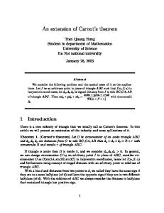
In order to illustrate the application of the described finite-temperature EXX approach to metals we considered three selected metals: the alkali metal sodium 共Na兲, the alkali earth metal magnesium 共Mg兲, and aluminum 共Al兲. We calculated band structures and density of states. For comparison, corresponding finite-temperature LDA calculations were performed. For each metal we considered the most common phases at room temperature at experimental lattice constants see Table I, i.e., for Na body-centered cubic 共bcc兲, space ¯ m; for Mg hexagonal closest packing group no. 229, Im3 共hcp兲, space group no. 194, P63 / mmc; and for Al face¯ m. centered cubic 共fcc兲, space group no. 225, Fm3 Figures 1–3 show comparisons of the EXX and LDA band structures for sodium, magnesium, and aluminum, respectively. Below and at the Fermi level, no significant differences between LDA and EXX band structures are observed. For aluminum the band repulsions below the Fermi level are slightly but not significantly larger 共few meV兲 in the EXX than in the LDA band structure. LDA and EXX bands cross the Fermi level at almost exactly the same points in the Brillouin zone and all occupied LDA and EXX levels are qualitatively comparable, as expected. This similarity between LDA and EXX band structures is also observed for insulators.28 Above the Fermi level, in particular at higher energies, however, significant differences between the LDA and EXX band structures start to build up. These differences, in some cases, can have magnitudes of 0.5 up to 2.0 eV. For instance, consider the EXX eigenvalues close to 8 eV for the k-point H in sodium 共see Fig. 1兲 and for the k-point M of magnesium 共see Fig. 2兲. These EXX eigenvalues are higher by

155119-7

PHYSICAL REVIEW B 81, 155119 共2010兲

GREINER, CARRIER, AND GÖRLING 30

30 25

20

15

energy [eV]

energy [eV]

20

10

5

10

0 fcc-Al

LDA+VWN EXX+VWN 0

bcc-Na

-10 LDA+VWN EXX+VWN

-5 Γ

∆

H

N

Σ

Γ

Λ

P

W

L

Λ

Γ

∆

X

Z

W

K

FIG. 1. 共Color online兲 Comparison of LDA and EXX band structures 共evaluated at room temperature兲 for sodium. The zero energy level corresponds the Fermi level.

FIG. 3. 共Color online兲 Comparison of LDA and EXX band structures 共evaluated at room temperature兲 for aluminum. The zero energy level corresponds the Fermi level.

more than 1 eV compared to their LDA counterparts. At higher energies the differences can occasionally increase up to almost 2.0 eV, e.g., at the ⌫ point of sodium 共see Fig. 1兲. We emphasize that these shifts in the energies of unoccupied bands are of the same order as the band gap shifts observed in semiconductors and insulators.28 We observe also that

band repulsions are stronger in the EXX band structures far above the Fermi level. For instance, in aluminum, the singly degenerated bands at the ⌫ point between 16 and 20 eV in the EXX case exhibit a band repulsion about 0.5 eV larger than in the LDA case. Furthermore the positions of several band crossings are shifted in some cases to the left and/or to the right in the EXX band structures compared to the LDA band structures, due to larger band repulsion in the EXX band structures. This finding also is observed in semiconductor band structures, e.g., for germanium.28 We emphasize, however, that the described local variations in LDA and EXX band energies do not affect the general shape and appearance of the band structures of Na, Mg, and Al, i.e., band ordering remains the same in LDA and EXX. The corresponding DOS are shown in Fig. 4 for the LDA and the EXX case of the three considered metals. Convergence of the DOS with respect to Nk was accomplished for each of the metals with 25⫻ 25⫻ 25 k points and for Na with a halfwidth of ␴Na = 0.74 eV, for Mg with ␴Mg = 1.04 eV and for Al with ␴Al = 0.64 eV, respectively 关see Eq. 共47兲兴. Up to 1.0–2.0 eV below Fermi level, the LDA and EXX case do not show any significant differences as expected from the corresponding band structures. Around the Fermi level and above, small differences build up due to the exact treatment of the unoccupied states in EXX formalism. Hereby, the EXX DOS can differ up to 3% to 5% from the LDA DOS, consider for instance the deviation in sodium at 3 eV or in aluminum at 4 eV. In order to investigate the temperature dependence of the DOS we did LDA and EXX calculations for Al and Na at 100 K and at a temperature close to the melting point 共i.e., at 800 K for Al and at 350 K for Na兲. As expected, the resulting DOS did not change signifi-

15

energy [eV]

10

5

0

-5 LDA+VWN EXX+VWN

hcp-Mg -10 Γ

Σ

M

K

T

Γ

∆

A

FIG. 2. 共Color online兲 Comparison of LDA and EXX band structures 共evaluated at room temperature兲 for magnesium. The zero energy level corresponds the Fermi level.

155119-8

PHYSICAL REVIEW B 81, 155119 共2010兲

EXTENSION OF EXACT-EXCHANGE DENSITY…

into account spin-orbit effects, noncollinear spin, and magnetic effects in metals.

EFermi

0.7 0.6 0.5

fcc-Al

ACKNOWLEDGMENTS

0.4 0.3 0.2

This work was supported by the Alexander von Humboldt-Stiftung 共P.C.兲. The authors gratefully acknowledge the funding of the German Research Council 共DFG兲, which, within the framework of its “Excellence Initiative” supports the Cluster of Excellence “Engineering of Advanced materials” 共www.eam.uni-erlangen.de兲 at the University of Erlangen-Nuremberg.

LDA+VWN EXX+VWN

0.1 0 0.7 [eV-1]

0.5

g(ε)

0.6

0.3

hcp-Mg

0.4

APPENDIX: OCCUPATION NUMBERS

0.2 0.1

At first, we here briefly reconsider a derivation of expression 共28兲 for the occupation numbers f i of KS orbitals in the case of a grand canonical ensemble72 and then generalize this derivation to the case of the occupation numbers gij of pairs of KS orbitals. The occupation numbers f i are given by

0 0.7 0.6 0.5

bcc-Na

0.4

⬁

0.3

fi =

0.2

兺 兺 N=1

ZvKS,T,␮

n

s

i苸⌽N,n

0.1 0

KS exp关共− 1/kT兲共EN,n − ␮N兲兴

⬁

-12 -11 -10 -9 -8 -7 -6 -5 -4 -3 -2 -1

0

1

2

3

=1−

energy [eV]

兺 兺

N=1

KS exp关共− 1/kT兲共EN,n − ␮N兲兴

ZvKS,T,␮

n

s

i苸⌽N,n

FIG. 4. 共Color online兲 Comparison of the density of states per unit cell between sodium, magnesium and aluminum 共evaluated at room temperature for Nk = 25⫻ 25⫻ 25 and ␴Na = 0.74 eV, ␴Mg = 1.04 eV and ␴Al = 0.64 eV兲. Results for LDA and EXX are presented in each case. The zero energy level corresponds the Fermi level.

⬁

= 1 − e共1/kT兲共␧i−␮兲 兺

N=1

⫻

兺

KS exp关共− 1/kT兲共EN+1,n − ␮共N + 1兲兲兴

ZvKS,T,␮

n

s

i苸⌽N+1,n

cantly from the DOS at room temperature, i.e., changes never exceeded 2 ⫻ 10−4 eV. We conclude this section by emphasizing that the effect of the presented EXX method, compared to the LDA method clearly does not correspond to that of a “scissors” operator. More precisely, the observed stronger band repulsions and the band shifts locally modify the band structures, especially high above the Fermi level.

⬁

=1−e

共1/kT兲共␧i−␮兲

兺 兺 N=2 n

KS exp关共− 1/kT兲共EN,n − ␮N兲兴

ZvKS,T,␮ s

i苸⌽N,n ⬁

⬇1−e

共1/kT兲共␧i−␮兲

兺 兺 N=1 n

KS exp关共− 1/kT兲共EN,n − ␮N兲兴

ZvKS,T,␮ s

i苸⌽N,n

= 1 − e共1/kT兲共␧i−␮兲 f i . V. CONCLUDING REMARKS

Now having at hand a finite-temperature EXX method for solids and, in particular, for metals it seems interesting to investigate with the new method metals that are insufficiently described by conventional LDA or GGA method. For example, metals having d electron shells, such as copper or iron, so as to determine exchange effects on the copper d bandwidth. Another example may be f-shell metals such as any of the lanthanoids. In a next step the finite-temperature EXX approach presented here can be combined with the magnetization-current density functional theory of Refs. 78 and 79 in order to take

共A1兲

In the first line of Eq. 共A1兲 we sum up the probability weights of all KS determinants that contain the KS orbital ␾i. To obtain the second line of Eq. 共A1兲 we use that its sum is the same as one minus the sum of the probability weights of all KS determinants that do not contain the KS orbital ␾i. For the third line we exploit that a summation over all N-electron KS determinants that do not contain the KS orbital ␾i equals a summation over all N + 1-electron KS determinants that do contain the KS orbital ␾i because the addition of an electron in the orbital ␾i to an N-electron KS determinant not containing ␾i leads to an 共N + 1兲-electron KS determinant containing orbital

155119-9

PHYSICAL REVIEW B 81, 155119 共2010兲

GREINER, CARRIER, AND GÖRLING

␾i and because vice versa the removal of an electron in the orbital ␾i from an 共N + 1兲-electron KS determinant containing ␾i leads to an N-electron KS determinant not containing orbital ␾i. Furthermore the energy of the considered pairs of N- and 共N + 1兲-electron determinants differs by the eigenvalues ␧i of the orbital ␾i. The forth line of Eq. 共A1兲 follows from a simple change of the summation variable. The forth and the fifth line differ by the summation term for N = 1 only. This term equals 1 / ZvKS,T,␮, the inverse of the

grand partition function 共6兲, and approaches zero for a large average electron number N as it occurs in the treatment of a solid if a large enough number of k points and/or a large enough unit cell is taken into account and the chemical potential ␮ is adjusted such that the solid is neutral. Rearrangement of Eq. 共A1兲 leads to expression 共28兲 for the occupation numbers f i. The occupation numbers gij of pairs of KS orbitals are given by

s

⬁

gij =

KS − ␮N兲兴 exp关共− 1/kT兲共EN,n

兺 兺

N=2

ZvKS,T,␮

n

s

i苸⌽N,n j苸⌽N,n ⬁

=1−

KS exp关共− 1/kT兲共EN,n − ␮N兲兴

兺 兺 N=1

ZvKS,T,␮

n

⬁

−

KS exp关共− 1/kT兲共EN,n − ␮N兲兴

兺 兺 N=1

ZvKS,T,␮

n

s

i苸⌽N,n

⬁

+

兺 兺 N=1

KS exp关共− 1/kT兲共EN,n − ␮N兲兴

n

s

j苸⌽N,n

ZvKS,T,␮ s

i苸⌽N,n j苸⌽N,n

⬁

= fi + f j − 1 +

兺 兺 N=1

exp关共−

n

KS 1/kT兲共EN,n ZvKS,T,␮ s

− ␮N兲兴

i苸⌽N,n j苸⌽N,n ⬁

KS exp关共− 1/kT兲共EN+2,n − ␮共N + 2兲兲兴

兺

= f i + f j − 1 + e共1/kT兲共␧i+␧i−␮−␮兲 兺

N=1

ZvKS,T,␮

n

s

i苸⌽N+2,n j苸⌽N+2,n ⬁

兺

= f i + f j − 1 + e共1/kT兲共␧i+␧i−␮−␮兲 兺

N=3

KS exp关共− 1/kT兲共EN,n − ␮N兲兴

ZvKS,T,␮

n

s

i苸⌽N,n j苸⌽N,n ⬁

⬇ f i + f j − 1 + e共1/kT兲共␧i+␧i−␮−␮兲 兺

N=2

兺

KS exp关共− 1/kT兲共EN,n − ␮N兲兴

n

ZvKS,T,␮

= f i + f j − 1 + e共1/kT兲共␧i+␧i−␮−␮兲gij .

共A2兲

s

i苸⌽N,n j苸⌽N,n

In the step from the second to the third line of Eq. 共A2兲 we add and subtract one and use the third line of Eq. 共A1兲. The fifth and sixth line of Eq. 共A2兲 differ by the summation term for N = 2 that again equals 1 / ZvKS,T,␮, the inverse of the grand s partition function 共6兲 and approaches zero for large enough electron numbers as they are encountered in the treatment of solids. Rearrangement of Eq. 共A2兲 leads to fi + f j − 1 = fif j. 1 − e共1/kT兲共␧i+␧i−␮−␮兲

With Eq. 共A3兲 expression 共32兲 for the sum of Coulomb and exchange energy assumes the form U + Ex = 共1/2兲 兺 兺 f i f j关具ij兩ij典 − 具ij兩ji典兴 i

= 共1/2兲

冕

j

drdr⬘

␳0共r兲␳0共r⬘兲 − 共1/2兲 兺 兺 f i f j具ij兩ji典, 兩r − r⬘兩 j i

共A3兲

共A4兲

The occupation numbers gij of pairs of KS orbitals thus are just given by the product of the occupation numbers f i and f j of the KS orbitals i and j.

which suggests to define the Coulomb and exchange energies individually as

gij =

155119-10

PHYSICAL REVIEW B 81, 155119 共2010兲

EXTENSION OF EXACT-EXCHANGE DENSITY…

冕

␳0共r兲␳0共r⬘兲 兩r − r⬘兩

共A5兲

Ex = 共− 1/2兲 兺 兺 f i f j具ij兩ji典,

共A6兲

U = 共1/2兲

drdr⬘

and i

j

respectively. The evaluation of the Coulomb and exchange energy via Eqs. 共A5兲 and 共A6兲 is straightforward and just

1 R.

G. Parr and W. Yang, Density-Functional Theory of Atoms and Molecules 共Oxford University Press, Oxford, 1989兲. 2 R. M. Dreizler and E. K. U. Gross, Density Functional Theory 共Springer, Heidelberg, 1990兲. 3 W. Koch and M. C. Holthausen, A Chemist’s Guide to Density Functional Theory 共Wiley-VCH, New York, 2000兲. 4 B. G. Johnson, P. M. W. Gill, and J. A. Pople, J. Chem. Phys. 98, 5612 共1993兲. 5 K. Burke, J. P. Perdew, and Y. Wang, Electronic Density Functional Theory: Recent Progress and New Directions 共Plenum Press, New York, 1998兲. 6 J. P. Perdew and A. Zunger, Phys. Rev. B 23, 5048 共1981兲. 7 F. Della Sala and A. Görling, Phys. Rev. Lett. 89, 033003 共2002兲. 8 F. Della Sala and A. Görling, J. Chem. Phys. 116, 5374 共2002兲. 9 Q. Wu, P. W. Ayers, and W. Yang, J. Chem. Phys. 119, 2978 共2003兲. 10 D. P. Joubert, Phys. Rev. A 76, 012501 共2007兲. 11 A. Holas, Phys. Rev. A 77, 026501 共2008兲. 12 J. M. Galbraith and H. F. Schäfer, J. Chem. Phys. 105, 862 共1996兲. 13 N. Rösch and S. B. Trickey, J. Chem. Phys. 106, 8940 共1997兲. 14 M. Weimer, F. Della Sala, and A. Görling, Chem. Phys. Lett. 372, 538 共2003兲. 15 A. Görling, J. Chem. Phys. 123, 062203 共2005兲 and reference therein. 16 J. P. Perdew and M. Levy, Phys. Rev. Lett. 51, 1884 共1983兲. 17 L. J. Sham and M. Schlüter, Phys. Rev. Lett. 51, 1888 共1983兲. 18 L. J. Sham and M. Schlüter, Phys. Rev. B 32, 3883 共1985兲. 19 J. P. Perdew, in Density Functional Methods in Physics, edited by R. M. Dreizler and J. da Providencia 共Plenum, New York, 1985兲, p. 265. 20 O. Gunnarsson and K. Schönhammer, Phys. Rev. Lett. 56, 1968 共1986兲. 21 R. W. Godby, M. Schlüter, and L. J. Sham, Phys. Rev. Lett. 56, 2415 共1986兲. 22 R. W. Godby, M. Schlüter, and L. J. Sham, Phys. Rev. B 36, 6497 共1987兲. 23 K. Schönhammer and O. Gunnarson, J. Phys. C 20, 3675 共1987兲. 24 W. Knorr and R. W. Godby, Phys. Rev. Lett. 68, 639 共1992兲. 25 A. Görling and M. Levy, Phys. Rev. A 52, 4493 共1995兲. 26 M. Grüning, A. Marini, and A. Rubio, Phys. Rev. B 74, 161103共R兲 共2006兲. 27 M. Grüning, A. Marini, and A. Rubio, J. Chem. Phys. 124, 154108 共2006兲. 28 M. Städele, M. Moukara, J. A. Majewski, P. Vogl, and A. Gör-

requires a simple generalization of whatever procedure is used to calculate Coulomb and exchange energy in a ground state EXX approach. The expressions for the occupation numbers gij and for the Coulomb and exchange energy given in Eqs. 共A3兲, 共A5兲, and 共A6兲 are those that are suggested by naive guess. However, it seems preferable to give the expressions a firm formal basis by deriving them starting from the basic finitetemperature KS formalism.

ling, Phys. Rev. B 59, 10031 共1999兲. R. T. Sharp and G. K. Horton, Phys. Rev. 90, 317 共1953兲. 30 J. D. Talman and W. F. Shadwick, Phys. Rev. A 14, 36 共1976兲. 31 V. Sahni, J. Gruenebaum, and J. P. Perdew, Phys. Rev. B 26, 4371 共1982兲. 32 V. R. Shaginyan, Phys. Rev. A 47, 1507 共1993兲. 33 A. Görling and M. Levy, Phys. Rev. A 50, 196 共1994兲. 34 A. Görling and M. Levy, Int. J. Quantum Chem. 56 共Quantum Chem. Symp. 29兲, 93 共1995兲. 35 T. Kotani, Phys. Rev. Lett. 74, 2989 共1995兲. 36 A. Görling, Phys. Rev. B 53, 7024 共1996兲; 59, 10370共E兲 共1999兲. 37 M. Städele, J. A. Majewski, P. Vogl, and A. Görling, Phys. Rev. Lett. 79, 2089 共1997兲. 38 T. Grabo, T. Kreibich, S. Kurth, and E. K. U. Gross, in Strong Coulomb Correlations in Electronic Structure: Beyond the Local Density Approximation, edited by V. I. Anisimov 共Gordon & Breach, Tokyo, 1998兲. 39 E. Engel and R. M. Dreizler, J. Comput. Chem. 20, 31 共1999兲. 40 A. Görling, Phys. Rev. Lett. 83, 5459 共1999兲. 41 S. Ivanov, S. Hirata, and R. J. Bartlett, Phys. Rev. Lett. 83, 5455 共1999兲. 42 A. Görling, Phys. Rev. Lett. 85, 4229 共2000兲. 43 S. Hamel, M. E. Casida, and D. R. Salahub, J. Chem. Phys. 114, 7342 共2001兲. 44 L. Veseth, J. Chem. Phys. 114, 8789 共2001兲. 45 S. Hirata, S. Ivanov, I. Grabowski, R. Bartlett, K. Burke, and J. D. Talman, J. Chem. Phys. 115, 1635 共2001兲. 46 W. Yang and Q. Wu, Phys. Rev. Lett. 89, 143002 共2002兲. 47 Q. Wu and W. Yang, J. Theor. Comput. Chem. 2, 627 共2003兲. 48 S. Kümmel and J. P. Perdew, Phys. Rev. Lett. 90, 043004 共2003兲. 49 R. J. Magyar, A. Fleszar, and E. K. U. Gross, Phys. Rev. B 69, 045111 共2004兲. 50 A. Qteish, A. I. Al-Sharif, M. Fuchs, M. Scheffler, S. Boeck, and J. Neugebauer, Comput. Phys. Commun. 169, 28 共2005兲. 51 P. Rinke, A. Qteish, J. Neugebauer, C. Freysoldt, and M. Scheffler, New J. Phys. 7, 126 共2005兲. 52 S. Sharma, J. K. Dewhurst, and C. Ambrosch-Draxl, Phys. Rev. Lett. 95, 136402 共2005兲. 53 D. R. Rohr, O. V. Gritsenko, and E. J. Baerends, J. Mol. Struct.: THEOCHEM 762, 193 共2006兲. 54 T. Heaton-Burgess, F. A. Bulat, and W. Yang, Phys. Rev. Lett. 98, 256401 共2007兲. 55 S. Sharma, J. K. Dewhurst, C. Ambrosch-Draxl, S. Kurth, N. Helbig, S. Pittalis, S. Shallcross, L. Nordström, and E. K. U. Gross, Phys. Rev. Lett. 98, 196405 共2007兲. 29

155119-11

PHYSICAL REVIEW B 81, 155119 共2010兲

GREINER, CARRIER, AND GÖRLING 56

P. Carrier, S. Rohra, and A. Görling, Phys. Rev. B 75, 205126 共2007兲. 57 A. Heßelmann, A. W. Götz, F. Della Sala, and A. Görling, J. Chem. Phys. 127, 054102 共2007兲. 58 C. Kollmar and M. Filatov, J. Chem. Phys. 128, 064101 共2008兲. 59 E. Engel and R. N. Schmid, Phys. Rev. Lett. 103, 036404 共2009兲. 60 E. Engel, Phys. Rev. B 80, 161205共R兲 共2009兲. 61 L. Hedin, Phys. Rev. 139, A796 共1965兲. 62 M. S. Hybertsen and S. G. Louie, Phys. Rev. B 34, 5390 共1986兲. 63 W. G. Aulbur, M. Städele, and A. Görling, Phys. Rev. B 62, 7121 共2000兲. 64 Time-Dependent Density Functional Theory, Lecture Notes in Physics Vol. 706, edited by M. A. L. Marques et al. 共Springer, Heidelberg, 2006兲. 65 P. Elliot, F. Furche, and K. Burke, Excited States from TimeDependent Density Functional Theory, Reviews in Computational Chemistry Vol. 26 共Wiley, New York, 2009兲, p. 91. 66 V. K. Staroverov, G. E. Scuseria, and E. R. Davidson, J. Chem. Phys. 124, 141103 共2006兲. 67 A. Görling, A. Heßelmann, M. Jones, and M. Levy, J. Chem.

Phys. 128, 104104 共2008兲. Heßelmann and A. Görling, Chem. Phys. Lett. 455, 110 共2008兲. 69 N. D. Mermin, Phys. Rev. 137, A1441 共1965兲. 70 M. Levy, Proc. Natl. Acad. Sci. U.S.A. 76, 6062 共1979兲. 71 M. Levy, Adv. Quantum Chem. 21, 69 共1990兲. 72 N. W. Ashcroft and N. D. Mermin, Solid State Physics 共Saunders, Philadelphia, 1976兲. 73 E. Engel, A. Höck, R. N. Schmid, R. M. Dreizler, and N. Chetty, Phys. Rev. B 64, 125111 共2001兲. 74 N. Troullier and J. L. Martins, Phys. Rev. B 43, 1993 共1991兲. 75 D. Lide, CRC Handbook of Chemistry and Physics 共CRC Press, Boca Raton, 1995兲. 76 S. H. Vosko, L. Wilk, and M. Nusair, Can. J. Phys. 58, 1200 共1980兲. 77 O. Madelung, Semiconductor Data Handbook 共Springer, Berlin, 1995兲. 78 S. Rohra and A. Görling, Phys. Rev. Lett. 97, 013005 共2006兲. 79 S. Rohra, E. Engel, and A. Görling, arXiv:cond-mat/0608505 共unpublished兲. 68 A.

155119-12