Heterogeneity and Long-Run Changes in U.S. Hours and the Labor Wedge Simona E. Cociuba

Alexander Ueberfeldt

University of Western Ontario

Bank of Canada

June, 2012 Abstract From 1980 until 2007, U.S. average hours worked increased by thirteen percent, due to a large increase in female hours. At the same time, the U.S. labor wedge, measured as the discrepancy between a representative household’s marginal rate of substitution between consumption and leisure and the marginal product of labor, declined substantially. We examine these trends in a model with heterogeneous households: married couples, single males and single females. Our quantitative analysis shows that the shrinking gender wage gaps and increasing labor income taxes observed in U.S. data are key determinants of hours and the labor wedge. Changes in our model’s labor wedge are driven by distortionary taxes and non-distortionary factors, namely the cross-sectional di¤erences in households’ labor supply and productivity. We conclude that the labor wedge measured from a representative household model partly re‡ects inaccurate household aggregation. Keywords: Female and Male Labor Supply, Labor Wedge, Gender Wage Gap, Labor Income Taxation, Household Aggregation. JEL: E24, H20, H31, J22. We thank Jim Dolmas, Lutz Hendricks, Gueorgui Kambourov, Narayana Kocherlakota, Mark Wynne and Carlos Zarazaga for their helpful comments. The views expressed herein are those of the authors and not necessarily those of the Bank of Canada. y Corresponding author : Cociuba, University of Western Ontario, Department of Economics, Social Science Center, Room 4071, London, Ontario, Canada, N6A 5C2. E-mail: [email protected].

1

1

Introduction

From the early 1960s to 2007; U.S. average hours worked, de…ned as the total hours worked in the marketplace relative to the working-age population, increased by thirteen percent. During the same time period, the U.S. labor wedge, measured as the discrepancy between a representative household’s marginal rate of substitution between consumption and leisure and the marginal product of labor, declined substantially. These observations are puzzling from the perspective of a standard neoclassical growth model because they were accompanied by a signi…cant increase in U.S. e¤ective labor income taxes.1 Given higher taxes, a model such as Prescott (2004) predicts lower hours worked, and a higher labor wedge. In this paper, we show that allowing for heterogeneous households in an otherwise standard growth model is important for understanding the observed trends in U.S. hours and the labor wedge. Our analysis is motivated by the fact that all of the trend increase in U.S. market hours is due to women. Married women’s hours more than doubled since the early 1960s, while the hours of single women rose slightly. In contrast, the hours of single and married men declined. We consider a neoclassical growth model with three types of households: married couples, single women and single men. Women receive a lower hourly wage rate compared to men, due to lower productivity and discrimination (as suggested by Goldin (1992)). Moreover, the labor income of all households is taxed. In this model, reductions in gender wage gaps are key in accounting for the increase in women’s hours, the increase in aggregate hours and the decline in the labor wedge. The main contribution of our paper is to show how changes in hours at the individual level in the presence of increasing taxes and shrinking gender wage gaps translate into a trend decline in the labor wedge at the aggregate level. To derive the model’s implications for the labor wedge, we aggregate the intratemporal labor equilibrium conditions of all men and women in our model. The analytical expression obtained shows that the labor wedge 1

E¤ective labor income taxes are de…ned as a combination of consumption and labor income taxes, similar to Prescott (2004) and Shimer (2009). For more details, see Section 4:1.

2

depends not only on taxes, as suggested by Mulligan (2002), Prescott (2004), and Ohanian, Ra¤o, and Rogerson (2008), but also on other labor market variables such as gender wage gaps, female labor supply and aggregate labor supply. Higher taxes lead to an increase in the labor wedge, while shrinking gender wage gaps (re‡ecting lower discrimination or higher relative productivity of women or a combination of the two) result in a lower labor wedge. In our quantitative experiments, we evaluate the relative importance of these opposing forces in accounting for the long-run changes in the U.S. labor wedge and hours worked. Existing literature has shown that the labor wedge is an important contributor to changes in aggregate macroeconomic variables (see Chari, Kehoe, and McGrattan (2007)).2 Several studies suggest that important determinants of the labor wedge are labor market distortions such as taxes, monopoly power, sticky wages, or search frictions (see e.g., Mulligan (2002), Chari, Kehoe, and McGrattan (2007), Shimer (2009)).3 In our heterogenous household model, the labor wedge is partly due to labor market distortions, such as taxes and discrimination, but partly due to non-distortionary factors, namely the cross-sectional di¤erences in households’labor supply and productivity. We conclude that the labor wedge measured from a representative household model partly re‡ects inaccurate aggregation across di¤erent types of households. Chang and Kim (2007) establish a similar result for cyclical ‡uctuations in the labor wedge in a heterogeneous-agent economy with incomplete capital markets and indivisible labor. In contrast to their paper, our analysis focuses on trend changes in the labor wedge in a model with gender and marital status heterogeneity. Our quantitative results show that changes in the relative productivity of men and women and changes in discrimination contribute to signi…cant reductions in the U.S. labor wedge.4 A calibrated version of our baseline model— with gender wage gaps and taxes measured from 2

Several other studies underscore the importance of the labor wedge in understanding economic ‡uctuations. See, for example, Ahearne, Kydland, and Wynne (2006) for a study of Ireland’s recession in the 1980s, Kersting (2008) for a study of the 1980s recession in the United Kingdom, or Chakraborty (2009) for an analysis of the labor wedge in Japan’s lost decade during the 1990s. 3 Parkin (1988) and Hall (1997) consider models with time-varying preferences and attribute changes in the labor wedge to shifts in preferences. 4 Cociuba and Ueberfeldt (2008) show that the decline in the Canadian labor wedge since early 1960s can also be accounted for by observed reductions in the gender wage gaps.

3

U.S. data— accounts for 63 percent of the increase in average hours worked, 86 percent of the increase in married women’s hours and about 30 percent of the decline in the labor wedge. The increase in taxes observed in the U.S. economy hurts our model’s predictions for both hours and the labor wedge. A variation of our baseline model in which taxes are held constant accounts for virtually all of the increase in aggregate and women’s hours and half of the decline in the labor wedge. We note that the model does not account for all of the decline in the labor wedge, since it has di¢ culty capturing the increase in the consumption to output ratio observed in the U.S. since the mid 1980s. Our paper relates to the literature examining taxation and long-run changes in labor supply. Prescott (2004) and Ohanian, Ra¤o, and Rogerson (2008) show that most of the variations in hours worked over time and across countries can be accounted for by di¤erences in taxes. High levels of hours worked are typically observed in countries or in periods of time in which labor income taxes are low. The U.S. is an exception, as both tax rates and hours worked increased since 1960s.5;6 Our paper shows that incorporating female labor and shrinking gender wage gaps allows an otherwise standard macroeconomic model to capture the observed increase in U.S. hours, even in the presence of higher taxes. Our results complement the literature that has focused on the importance of gender wage gaps to women’s labor supply (see e.g., Goldin (1992), Jones, Manuelli, and McGrattan (2003), Bar and Leukhina (2011) and Attanasio, Low, and Sánchez-Marcos (2008)). We consider some extensions of our analysis and their implications for hours and the labor wedge. Following Attanasio, Low, and Sánchez-Marcos (2008), we augment our model in order to quantify the impact of decreasing child care costs on women’s labor supply. We 5

Scandinavian countries are another exception, see Ragan (2006) and Rogerson (2007). Several hypotheses have been put forward to account for the U.S. labor supply data. Prescott (2004) suggests that the ‡attening of the income tax rate schedule in the 1980s plays an important role in accounting for the increase in U.S. labor supply. He conjectures that reductions in the marginal tax rate for two-earner households led to the observed rise in female participation and thus a rise in aggregate labor supply. However, Bar and Leukhina (2009) show that the tax reforms of 1980s had only a small e¤ect on married females participation and conclude that other factors were more important. Ohanian, Ra¤o, and Rogerson (2008) suggest that changes in time devoted to home production may be important for the U.S. We discuss this in more detail in Section 5:2. 6

4

…nd that reductions in this cost lead to increases in married women’s hours and in aggregate hours. Quantitatively, this complements the predictions obtained from a model without child care costs, although we …nd the shrinking of the gender wage gaps to be more important. Moreover, we discuss the importance of taking changes in home production and leisure time into account, as suggested by Ohanian, Ra¤o, and Rogerson (2008). We show that while it helps improve the predictions of the model, this mechanism alone cannot account for all of the changes in U.S. hours and the labor wedge. The paper is organized as follows. Section 2 documents the trend changes in U.S. hours and the labor wedge. Using a simple model, we illustrate that taking heterogeneity of the population into account is important for understanding these trends. Section 3 presents our baseline model with gender and marital status heterogeneity. We derive the analytical expression for the model’s labor wedge and discuss brie‡y the model’s predictions for hours and the labor wedge. Section 4 presents the quantitative experiments and results. In Section 5; we consider other factors— such as changes in child care costs, leisure time and time devoted to home production— and discuss their relative importance for the trends observed in U.S. hours and the labor wedge. We conclude in Section 6.

2

U.S. Data and a Simple Static Model

In this section, we …rst document the trends in U.S. hours and the labor wedge. Then, we use a simple model to illustrate that taking into account heterogeneity of the population is important for understanding these trends.

2.1

A Look at U.S. Data

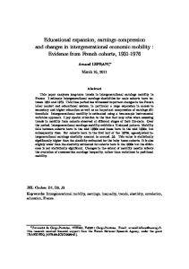
The changes in the aggregate weekly hours worked in the U.S. economy from 1961 to 2007 are documented in the upper left panel of Figure 1 (see Appendix A:1 for details on the data sources and computations). Throughout the 1960s and the 1970s, the U.S. working-age

5

population worked, on average, 25 hours per week. Beginning in the early 1980s, aggregate hours increased steadily to 28 hours per week in 2007:7 The upper right panel of Figure 1 plots the average weekly hours worked for males and females, by marital status. We see that the increase in aggregate hours is driven by women. In 1961; married men worked an average of 39 hours per week, while single men worked 28 hours, single women worked 22 hours and married females worked only 10 hours. By 2007; men’s hours declined by 4 to 10 percent, while women’s hours increased. The largest increase was in the hours of married women, which more than doubled over the 47 year period. These di¤erences in the hours worked by men and women motivate our general model in Section 3. The bottom panel of Figure 1 plots the labor wedge for the U.S. economy, normalized to equal 1 in year 1961. We follow the literature and measure the labor wedge using aggregate U.S. data and the intratemporal labor equilibrium condition from the neoclassical growth model with a representative household (see e.g., Parkin (1988), Hall (1997), Mulligan (2002), Chari, Kehoe, and McGrattan (2007) and Shimer (2009)). In this model, the time allocation decision is based on a static condition which equates the marginal product of labor (M P L) to the marginal rate of substitution between consumption and leisure (M RS). We use U.S. data to measure the M P L and the M RS, and obtain the labor wedge as the residual that makes the model condition hold in the data. Many macroeconomic studies (including, but not limited to, the ones cited above) use a Cobb-Douglas production function. Then, the M P L can be written as (1

) yt =lt ; where yt denotes output per person, lt denotes aggregate

hours worked per person and 1

is the labor income share. Time separable log preferences

in consumption and leisure— frequently used in macroeconomic studies— give a M RS equal to

(ct + gt ) = (1

lt ) ; where ct denotes private consumption per person, gt denotes public

consumption per person,

is the leisure utility parameter and

measures the marginal rate

of substitution between government and private consumption. With these functional forms, 7

U.S. aggregate hours worked have declined during the most recent recession, dated by the NBER to last from December 2007 to June 2009. The changes in hours observed since 2007 are interesting in their own right, but are not analyzed in this paper.

6

the labor wedge,

t;

is computed as follows:

1

(ct + gt ) 1 lt

t

where ct ; gt ; yt ; lt are taken from U.S. data, (2004)) and

=

(1

) yt lt

equals 0:33,

(1)

is close to 1:6 (as in Prescott

equals 1 (as in Prescott (2004) and Ohanian, Ra¤o, and Rogerson (2008)).8

As seen in Figure 1; the U.S. measured labor wedge is fairly constant for the period 1961 to 1980; and shows a trend decline between the early 1980s and 2007: This substantial decline in the labor wedge is also documented in Mulligan (2002) and Shimer (2010), under di¤erent functional forms for the marginal value of time (M RS).

2.2

Heterogeneity and the Labor Wedge

We illustrate that heterogeneity is important for understanding the trend decline in the labor wedge. We present a simple static model with households of di¤erent productivities to build intuition for this result. We show that the labor wedge is partly due to crosssectional di¤erences in the productivities of households. An immediate implication is that changes in the labor wedge are not entirely driven by labor market distortions, such as taxes, but also re‡ect changes in non-distortionary factors, such as the labor supplies and relative productivities of various sub-groups of the population. In other words, the labor wedge measured from a representative household model re‡ects inaccurate aggregation. The simple economy consists of di¤erent types of households indexed by j: Each household has one member who is endowed with one unit of time and has a …xed amount of capital given by kj . Households supply labor in the market, but di¤er in their productivity, which

8

The values of the parameters ;

and

are discussed in more detail in our quantitative results section.

7

is denoted by zj : The maximization problem solved by household j is:

max log (cj + g) + cj ;lj

subject to: cj

rkj + (1

log (1

lj )

l ) wzj lj

+

j

The utility is de…ned over private consumption, cj ; government consumption per person, g, and leisure time, 1 rameters

and

lj , where lj is the fraction of available time devoted to work. Pa-

are de…ned as before, in Section 2:1. Households receive wage rate w per

unit of e¤ective labor, zj lj ; and capital income rkj for renting the capital stock to the …rm: Labor income is taxed at rate

l;

and

j

are lump-sum transfers from the government.

~ to produce output accordThe representative …rm uses capital, K; and e¤ective labor, L; ~ 1 :9 Here, A denotes the total ing to the Cobb-Douglas production function: Y = AK L P factor productivity, K is the capital stock given by K = j kj and the e¤ective labor is ~ = P (zj lj Nj ) ; where Nj represents the number of households of type j. The given by L j

wage rate per unit of e¤ective labor is given by w = (1 ) y=~l; where y = Y =N is the output P ~ is the aggregate e¤ective labor per person, N = j Nj is the total population and ~l = L=N per person.

We show that in this simple model there exists a wedge between the aggregate marginal rate of substitution between consumption and leisure (M RS) and the marginal product of an hour worked (M P L). We start with the optimality condition which governs the consumption and time allocation decisions for each household j :

(cj + g) = (1

lj ) = (1

l ) wzj :

This

condition equates the marginal rate of substitution of household j to its after-tax marginal

9

We allow for capital stock in order for our derivations to be analogous to those presented in our general model in Section 3. However, the same intuition about the labor wedge presented in this section can be derived in an environment in which the production function uses only labor input.

8

product of labor. Aggregating across households, we obtain:10 (c + g) = (1 1 l P

where c

j

l)

X j

1 zj 1

lj Nj l N

!

l (1 ~l

)

y l

(2) P

cj Nj =N is aggregate private consumption per person, and l

j

(lj Nj ) =N

is aggregate hours worked per person, and where we have used the expression for the wage w: Using equation (2) ; the labor wedge,

1

(c + g) 1 l

= (1

; is given by: y ) l

= (1

l)

X j

1 zj 1

lj Nj l N

!

l ~l

(3)

As seen in equation (3), the labor wedge is partly due to distortionary taxes, but also re‡ects non-distortionary factors such as the di¤erent productivities and labor decisions of each household in the economy. We provide a numerical illustration to show that heterogeneity of the working population matters for the labor wedge. Consider an economy with two types of households of equal proportion in the population and without tax distortions (i.e. l

= 0). The labor supply, lj ; and productivity, zj ; of each type of household are presented

in Table 1. In the …rst scenario, there are large di¤erences in hours worked and productivity between the households. Type 2 households work only a quarter of the time per week and are 30 percent less productive compared to type 1 households. In this case, there is a wedge between the aggregate M RS and the M P L which is computed from equation (3) and equals 0.13. For smaller di¤erences in both hours and productivity (as shown in case 2, Table 1), the labor wedge remains positive, but shrinks to about 0.02. Finally, if all households work the same hours (as in case 3), or have the same productivity (as in case 4), and because l

= 0 in our example, the labor wedge disappears. This result holds more generally. When

lj = l for all j or when zj = z for all j; the labor wedge in equation (3) reduces to 1 10

l:

11

We multiply the individual optimality conditions by the fraction of agents of type j in the total populaP P tion, Nj =N; and sum up to get: lj ) (Nj =N ) w: Next, we substitute l) j (cj + g) Nj =N = (1 j zj (1 in the expression for the wage and divide both sides by (1 l). P P N 11 If lj = l for all j, then ~l = l (zj Nj ) =N: Using equation (3) ; 1 = (1 zj j l = (1 l) l) : j

j

9

N

~ l

Next, we present our general model with households that di¤er by marital status, gender, and productivity and show that changes in non-distortionary factors are important for understanding the decline in the U.S. labor wedge.

3

General Model

In order to examine changes over time in U.S. hours and the labor wedge, we consider a neoclassical growth model with three types of households: married couples, single females, and single males. The labor supply decisions of individuals are in‡uenced by several factors, of which the most important are gender wage gaps and e¤ective labor income taxes. Let Nt be the total population at time t. Let Npt ; Nf st ; and Nmst denote the total number of married couples, single females and single males, respectively. Similar to Jones, Manuelli, and McGrattan (2003), we assume that individuals in a married couple solve for decisions e¢ ciently. They choose streams of consumption, labor supply and investment to solve their joint decision problem with utility weights given by

max

1 X

t

[

f Uf

(cf pt + gt ; 1

f

and

lf pt ) +

m:

m Um

(cmpt + gt ; 1

lmpt )] Npt

t=0

subject to : cf pt + cmpt + xpt Npt+1 kpt+1 Npt

[(1

kt ) rt

xpt + (1

+

kt ] kpt

+ (1

lt ) wt

[lmpt + (1

pt ) lf pt ]

+

pt

) kpt

where subscripts f and m denote female and male, subscript p indicates a married couple or partnership, and t is the time subscript. The utility of a married individual of gender j 2 ff; mg is de…ned over streams of private consumption, cjpt ; average government consumption, gt ; and leisure time, 1

ljpt ; where available time is normalized to 1 and ljpt is the labor

supply expressed as the fraction of available time worked. The discount factor is

Similarly, if zj = z for all j; then ~l = zl and 1

=1

10

l:

2 (0; 1) :

The parameter

2 (0; 1) measures the marginal rate of substitution between private and

government consumption. The married couple owns capital stock, kpt ; which depreciates at rate

and is augmented by investments, xpt : The capital stock is rented to the …rm at

interest rate rt ; and the capital income net of depreciation is taxed at rate couple also pays taxes on labor income at rate pt :

lt ;

kt :

The married

and receives lump-sum transfers given by

12

In our model, married males receive an hourly wage rate of wt ; while married females receive only wt (1

pt )

per hour worked. Here,

pt

2 (0; 1) represents the gender wage gap

for married couples, which is exogenous to the model.13 Motivated by existing evidence, we assume that women receive a lower wage for two reasons: productivity di¤erences relative to men and discrimination. Goldin (1992) discusses in detail that some of the U.S. gender gap in earnings for various occupations can be explained by di¤erences in observable attributes between men and women, such as job experience, education. However a substantial part of the earnings gap remains unexplained and is attributed to discrimination.14 In our model, we assume that productivity di¤erences account for a fraction

2 [0; 1] of the gender wage

gap, while discrimination accounts for the remainder. In particular, the hourly wage rate received by a married woman can be written as:

wt (1

pt )

= wt (1

pt )

12

wt (1

)

pt

(4)

In our model, the e¤ective labor income tax (de…ned as in footnote 1) is the same for singles and married individuals, as well as for men and women. We have constructed estimates of average income taxes for single men, single women, married men and married women using the methodology in Kryvtsov and Ueberfeldt (2007). We …nd that while the level of the tax varies slightly, the increase in the income tax between 1961 and 2001 is comparable across groups. Moreover, as discussed in footnote 6, Bar and Leukhina (2009) …nd that the U.S. tax reforms of 1980s have a small e¤ect on married females participation. For these reasons, we do not consider di¤erent tax rates for the di¤erent households in our model. 13 A few studies in the literature endogenize the gender wage gap. Erosa, Fuster, and Restuccia (2002, 2005) endogenize the married women’s gender wage gap, by relating it to the human capital lost after child birth. In Jones, Manuelli, and McGrattan (2003) the gender wage gap is partly endogenous, due to human capital decisions, and partly exogenous, due to direct wage discrimination or to the existence of a “glass ceiling” that keeps women from rising in the hierarchy of organizations. 14 For example, Goldin (1992) documents that wage discrimination was about 20 percent of the di¤erence in male and female earnings in manufacturing jobs in early 1900, and about 55 percent for o¢ ce work in 1940:

11

where wt (1

pt )

is the wage rate women should receive given their marginal product

of labor (i.e. taking into account productivity di¤erences relative to men), while the term wt (1

)

pt

represents the portion of the wage rate lost due to discrimination. Measures of

wage discrimination from U.S. data— such as those discussed in Goldin— vary over time. For simplicity, we consider that the fraction of the gender gap accounted for by discrimination is constant over time in the model and is given by 1

. In Section 4; we evaluate the

importance of this assumption for female hours and the U.S. labor wedge by presenting results under two extreme scenarios: the gender wage gap is due entirely to discrimination or due entirely to productivity di¤erences. For

2 (0; 1), our model is consistent with the view that reductions in the gender

gap observed in the U.S. since the early 1960s; were a consequence of improvements in productivity of women and reductions in discrimination. As seen in equation (4), when the gender wage gap, wt (1

pt ),

pt ;

shrinks over time, the marginal product of a married woman’s labor,

increases, while the wages lost due to discrimination, wt (1

)

pt ;

decline.

Single males and females solve the following maximization problem:

max

1 X

t

Uj (cjst + gt ; 1

ljst ) Njst

t=0

subject to cjst + xjst Njst+1 kjst+1 Njst

: [(1

kt ) rt

xjst + (1

+

kt ] kjst

+ (1

lt ) wt

(1

Ij

st ) ljst

+

jst

) kjst

where, as before, subscripts j 2 ff; mg and t denote gender and time, and subscript s indicates a single individual. We use similar notational conventions as in the married couple’s problem. The indicator function Ij equals 1 if j = f and zero otherwise and is used to show that single males receive hourly wage rate wt ; while single females receive (1 st

st ) wt :

2 (0; 1) represents the gender wage gap for singles. As before, the parameter

Here,

governs

the share of the gender wage gap accounted for by productivity di¤erences. In our numerical

12

experiments, the gender wage gap for singles, pt ,

st ,

di¤ers from the one for married couples,

consistent with U.S. data.

Our model di¤erentiates between males and females along two main dimensions. First, married and single females receive a lower wage than males. In the quantitative experiments, we allow the gender wage gap for singles and for married couples to di¤er, as in the data. As we show in later sections of the paper, reductions in the gender wage gap are important in accounting for the increase in female hours worked over time. The second di¤erence between males and females in our model exists only for married couples and consists of the di¤erent utility weights

f

and

m

1

f:

In the quantitative experiments, the parameter

f

determines the relative level of hours worked for married men and women in the …rst period of our model (for details see Section 4). There is a representative …rm with a constant returns to scale production function that ~ t . The …rm’s problem is: rents capital, Kt ; and pays for e¤ective labor, L ~t max F Kt ; L

r t Kt

~t = K subject to: F Kt ; L t

~t wt L ~

(5) 1

t Lt

There is labor augmenting technical progress at a constant yearly rate of t

=

0

t

1; that is,

. The aggregate resource constraints for capital and e¤ective labor are given by:

Kt = kpt Npt + kf st Nf st + kmst Nmst ~ t = lmpt Npt + (1 L

pt ) lf pt Npt

+ (1

st ) lf st Nf st

+ lmst Nmst

~ t : Here, wt is the wage rate per unit of e¤ective The wage bill in (5) is given by wt L ~ t ; the terms labor and also the wage rate per hour worked by men. In the expression for L (1

it )

for i 2 fp; sg measure the productivity of a married or single woman relative to

men. Recall that women do not get paid their marginal product of wt (1

13

it ),

but receive

the lower hourly wage rate of wt (1

it )

due to discrimination (as seen in equation (4) for

married women). The di¤erence between their marginal product and the wage rate received is equal to wt (1

)

it ;

and is collected by the government as revenue from discrimination.

~ t = Ct + Xt + Gt ; where The resource constraint in the economy is given by: F Kt ; L aggregate consumption is Ct is Xt

Npt (cmpt + cf pt ) + Nmst cmst + Nf st cf st ; aggregate investment

Npt xpt + Nmst xmst + Nf st xf st and Gt

Nt gt denotes government spending. In the

quantitative analysis, the government consumption is exogenous and is allowed to vary over time. The government collects revenue from discrimination and from capital and labor income taxation. The revenue is used for government consumption expenditures and the remainder is lump-sum rebated to households. The lifetime budget constraint of the government is given by: 1 X 1

(

where

Nmst

mst ;

(1

t

kt ) rt

+

lt wt Npt lmpt

+ [wt (1

)

+

kt rt

Q > : t&=1 (1 kt ;

kt ] Kt

+ R& ) for t

+ wt (1

(6)

0

aggregate transfers are

+

tg

+

for t = 0

1

lt wt Nmst lmst

pt Npt lf pt

f[

t

t=0

8 > <

and aggregate labor revenues,

[

t

+ Gt ) =

t

t=0

and where, Rt

t

1 X 1

Npt

t

pt

+ Nf st

f st

+

are de…ned as:

t;

lt

(1 )

pt ) wt Npt lf pt

+

lt

(1

st ) wt Nf st lf st ] (7)

st Nf st lf st ]

Both men and women pay taxes on their labor income at rate

lt .

The revenues collected

from this tax are given by the …rst four terms in equation (7) : In addition, women’s labor income is subject to discrimination which raises revenues equal to wt (1 wt (1

)

st Nf st lf st .

14

)

pt Npt lf pt

+

In our quantitative experiments, we allow the e¤ective labor income taxes, wage gaps, Npt =Nt ; nf st

st

and

pt ;

lt ;

the gender

the government consumption, gt ; and the population fractions, npt

Nf st =Nt ; nmst

Nmst =Nt ; to vary exogenously over time. We allow the

population fractions to vary since there has been a large increase in the fraction of singles and a corresponding decline in the fraction of married couples since 1961: All time-varying inputs are measured from U.S. data, as discussed in Section 4:

3.1

Hours and the Labor Wedge in the Model

Our model augments the representative household growth model presented in Prescott (2004) and Ohanian, Ra¤o, and Rogerson (2008) by considering labor supply decisions of men and women. In this section, we discuss why this extension brings the model’s predictions closer to data. We also discuss brie‡y the counterfactual predictions of a representative household model for U.S. hours and the labor wedge. Our quantitative results are shown in Section 4. 3.1.1

Hours Worked

We brie‡y discuss a few determinants of hours worked in our model. More details are provided in the results section. Households in our model own the capital and rent it to the …rm. Equivalently, we could allow the …rm to buy the initial capital from the household and make capital investments thereafter. In other words, the consumption and labor supply decisions of households do not depend on who makes the capital investment. However, these decisions are a¤ected by the household’s initial wealth and the lump-sum transfers it receives over the lifetime. To illustrate this, we aggregate the sequential budget constraints of singles of gender j 2 ff; mg

15

into the following lifetime budget constraints. 1 X

Njst

t=0

1 t

cjst

1 X

Njst

t=0 1 X

+

t

(1

lt ) wt

(1

Ij

(8)

st ) ljst

t

Njst

t=0

where

1

1 t

jst

+ Njs0 (1

+ (1

k0 ) r0

+

k0 ) kjs0

is de…ned as in (6) and Ij = 1 if j = f and zero otherwise:

A similar lifetime budget constraint can be derived for the married couple as well. We see from equation (8) that aggregate lifetime transfers and the initial wealth due to the ownership of the capital stock in‡uence the lifetime income of households, and thus, have an e¤ect on the level of hours worked. Large lifetime transfers result in lower equilibrium hours for the household. A key di¤erence between the individuals in our model is the hourly wage rate they receive. If the gender wage gaps are zero (i.e. everyone receives the same wage and is equally productive), the men and women in our model make the same choices provided that (i) initial wealth and lifetime transfers are proportional to the lifetime labor income of each household and (ii) the individuals in the married couple have equal utility weights:

m

=

f:

Under

these conditions, the model reduces to a representative household model with labor income taxes as in Prescott (2004) and Ohanian, Ra¤o, and Rogerson (2008). Then, the model predicts that everyone’s hours are the same lf pt = lf st = lmst = lmpt for all t: Moreover, an increase in the e¤ective labor income tax leads to a decline in everyone’s hours and, thus, in aggregate hours. This is consistent with the results of the two previous studies mentioned, but inconsistent with U.S. data which shows an increase in hours worked despite an increase in e¤ective labor income taxes,

lt

(see Section 4.1 for details).

The model delivers more interesting predictions for hours worked when gender wage gaps are positive. All else equal, women in the model work fewer hours than men, and their hours grow over time as the gender wage gaps shrink. Both of these predictions are consistent with U.S. data. In Section 4, we evaluate the quantitative importance of taxes, gender wage gaps 16

and other model features in accounting for the changes in U.S. hours worked. 3.1.2

Aggregation and the Labor Wedge

We derive the labor wedge in our model and show that it depends on taxes, as suggested by previous studies, but also on labor market variables such as gender wage gaps, female labor supplies and the aggregate labor supply. The derivation is similar to that in Section 2. To obtain an expression for the labor wedge we aggregate the model’s labor equilibrium conditions which are summarized in equation (9) for married and single men and in equation (10) for married and single women. (cmit + gt ) = (1 1 lmit (cf it + gt ) = (1 1 lf it

lt ) wt ; lt ) (1

for i 2 fp; sg it ) wt ;

(9)

for i 2 fp; sg

(10)

We multiply each of the intratemporal conditions by the fraction of households of that type (i.e. fraction of married couples, npt ; and fraction of singles, nf st and nmst ) and sum up to obtain equation (11) :15 (ct + gt ) = (1 1 lt

lt )

1

npt

pt

(1

lf pt ) + nf st 1 lt

st

(1

lf st )

(1

) yt ~lt

(11)

Here, ct = Ct =Nt denotes aggregate private consumption per person, gt = Gt =Nt denotes public consumption per person; lt = npt lmpt + npt lf pt + nmst lmst + nf st lf st denotes aggregate ~ t =Nt denotes aggregate e¤ective hours per person and yt = hours worked per person, ~lt = L ~ t =Nt denotes output per person. F Kt ; L Combining equation (11) with the de…nition of the labor wedge given in equation (1) ; we can rewrite 1

t

as in (12) :

1

t

= (1

15

lt )

1

npt

pt

(1

For a full derivation, see Appendix A:2.

17

lf pt ) + nf st 1 lt

st

(1

lf st ) lt ~lt

(12)

The labor wedge,

t;

depends on endogenous labor supply decisions of the households,

as well as time-varying exogenous inputs of the model such as taxes, gender wage gaps and fractions of females in the total population. Notice that — the parameter the governs the share of the gender wage gap accounted for by productivity di¤erences— enters equation (12) indirectly through ~lt : When

= 1; the gender gap is due entirely to productivity di¤erences

between men and women. Then, changes in the labor wedge re‡ect changes in distortionary taxes, as well as changes in non-distortionary factors, such as the productivity of women, as discussed in the static example in Section 2. When

= 0; the gender gap is due entirely to

discrimination which can be interpreted as another distortion that a¤ects the changes in the labor wedge. In what follows, we brie‡y discuss the model’s predictions for the labor wedge under various scenarios. A more detailed analysis is provided in the quantitative experiments section. First, consider the case when men and women earn the same wage (i.e. Equation (12) simpli…es to: 1

t

= 1

lt ;

pt

=

st

= 0).

which means that the model’s labor wedge

is exogenously determined. As discussed in Section 3:1:1, the model reduces to a standard growth model with taxes, as in Prescott (2004) and Ohanian, Ra¤o, and Rogerson (2008). Since taxes,

lt ;

increased in U.S. data in the last 50 years, the labor wedge,

t;

generated

under this scenario increases, contrary to what was observed in U.S. data. Now consider the more interesting case in which the gender wage gaps are positive (i.e. pt

> 0;

st

> 0). For simplicity, assume that our model has only married couples and no

single households, and that the gender wage gap is due entirely to discrimination. Equation (12) simpli…es to: 1

t

= (1

lt ) [1

0:5

pt

(1

lf pt ) = (1

lt )] : Can the model

deliver a labor wedge that declines over time as seen in U.S. data? Recall that since the early 1960s; the U.S. gender wage gap shrunk and taxes increased. If the model generates an increase in aggregate hours, lt ; and a larger increase in female hours, lf pt ; the term [1

0:5

pt

(1

lf pt ) = (1

lt )] increases over time. In our quantitative analysis, we show

that this increase dominates the decline in (1

18

lt ) ;

and the model delivers a decline in the

labor wedge,

4

t;

over time (see Section 4:2 for details).

Quantitative Analysis

We compute the equilibrium paths of our model and compare its predictions with U.S. data. In our baseline experiment, we treat the e¤ective labor income taxes, the gender wage gaps, the government consumption and population fractions as exogenous, time-varying inputs. We perform other experiments to isolate the quantitative importance of each factor.

4.1

Baseline Calibration

Here, we present and motivate the model parameters and the exogenous series used as inputs in the quantitative experiments. We choose parameters so that our baseline model matches key statistics of the U.S. economy. We use national accounts and …xed assets data, revenue statistics and survey data for the U.S. as described in detail in Appendix A:1. Unless otherwise noted, we use data for the years 1961 to 2007: The parameters and time-varying inputs are summarized in Figure 2 and Table 2. First, we discuss the measurement of the time-varying exogenous inputs of our model. The e¤ective labor income taxes are de…ned as in Prescott (2004) and Shimer (2009). In particular,

lt

=1

(1

ht ) = (1

+

ct ) ;

where

ht

and

ct

are the labor income tax rate

and the consumption tax rate which are constructed following the methodology of Mendoza, Razin, and Tesar (1994). The interpretation of this e¤ective tax is that one additional unit of pre-tax labor income buys (1

ht ) = (1

+

ct )

units of consumption, after labor and

consumption taxes are paid for. The government-consumption to output ratio is constructed using national accounts data. The gender wage gaps for married and single individuals, and

st ;

pt

are measured using microdata from the Current Population Survey (CPS) as detailed

in the data appendix. Finally, the population fractions, npt ; nf st ; nmst ; are also measured from the CPS.

19

We choose

to match the average population growth rate and

to match the average

growth rate of labor augmenting technical change over the 47 year period. We choose

and

to match the average capital income share and the average depreciation rate, respectively. We set

k

to the average capital income tax for the U.S. since 1970: The discount factor is

chosen to match a steady state after-tax net return (1 We use the following utility function: Uf = Um = U =

+ k of 4 percent. n o 1 [(c + g) (1 l) ] 1 :

k) r 1 1

We follow Prescott (2004) and Ohanian, Ra¤o, and Rogerson (2008) and set the intertemporal substitution parameter, leisure parameter, 1

m

f;

; and the government consumption parameter,

; to 1. The

; and the utility weights in the married couple’s problem,

are calibrated as follows. First, note that

f

and

a¤ects the level of hours of

all individuals in the economy, as well as the level of aggregate hours. The utility weights f

and

and

f

m

in‡uence the relative level of hours for married males and females. We pick

so that the aggregate labor supply and married female labor supply in the initial

period in the model are consistent with U.S. data on hours worked in 1961. Recall that labor supply in the model is expressed as a fraction of available time worked. Given 100 hours of available time per week, the aggregate weekly hours worked in the model are lt 100 and married female weekly hours worked are lf pt 100: Our calibration ensures that l1961 100 equals 24:6 hours and lf p1961 100 equals 10:3 hours, as observed in U.S. data in 1961. Once and

f

are calibrated, the levels of hours for the other individuals for the year 1961 are

determined in equilibrium. As discussed in Section 3:1:1, the initial capital stock wealth and lifetime transfers have an impact on the level of hours of each household. We set initial wealth of each household, kp0 ; kf s0 and kms0 ; to be proportional to labor income in 1961: We set lifetime transfers to be proportional to the total income (labor income plus initial capital stock wealth) earned by each household in the model. This choice of distributing transfers preserves the ratios of lifetime income between the three groups of households. In our baseline calibration, we assume that the gender gap is entirely due to discrimination

20

(i.e.

= 0). We later perform a sensitivity analysis to this choice by considering how our

results change when the gender gap is accounted for entirely by productivity di¤erences between males and females (i.e.

4.2

= 1) :

Results

We evaluate the extent to which the model is able to replicate trends in average hours worked for the di¤erent population groups relative to the U.S. data. We measure the labor wedge generated in the model— as the aggregate discrepancy between the marginal rate of substitution between consumption and leisure and the marginal product of labor— and examine whether it is consistent with U.S. data. We report results from multiple experiments in order to isolate the relative importance of the di¤erent factors considered: taxes, gender wage gaps, government consumption ratio and population fractions. In Section 5, we discuss other factors that may be important for labor supply, such as child care costs, home production and leisure time. Our baseline model allows all exogenous inputs— taxes, gender wage gaps, government consumption ratio and population fractions— to vary over time as seen in U.S. data (see Figure 2). The results for hours worked and the labor wedge are reported in Figure 3. The solid lines in the left side panels of the …gure show weekly hours worked by males and females in the U.S. economy between 1961 and 2007: The dashed lines show the baseline model results for hours worked (e.g. for married males, we plot lmpt 100 where lmpt is the fraction of time worked and 100 represents the available hours per week). The model is successful in matching the level of hours and in accounting for the changes in hours over time. Recall that aggregate hours and married females hours for the year 1961 are matched through the choice of f.

and

The levels of hours worked for married males, single males and single females for the year

1961 are not pinned down in the calibration, but are determined in equilibrium. While the model does not match these levels exactly, it does deliver the same ranking of hours among the di¤erent population groups as in the data for the year 1961. For example, in the data, a 21

single male worked about 26% more than a single female in year 1961, while the comparable …gure in the model was 25%. The upper right panel of Figure 3 plots aggregate weekly hours worked in the data and in the baseline model (variable lt ). The model predicts correctly very little changes in hours between 1960 and 1980; and an increase in hours afterwards. In the data, the overall increase in hours since 1960 was 13:3 percent, while the model delivers an increase of 8:4%: An obvious discrepancy between the model and the data is seen during the 1990s: In the data, aggregate hours worked increase, while the model predicts a decline during this period due to the increase in observed taxes.16 Lastly, as seen in the lower right panel of Figure 3; the model delivers a decline in the labor wedge since the early 1980s. More detailed results from the baseline model are shown in Tables 3 and 4: Table 3 presents a detailed comparison of hours in the data and the model. Using the expression for lt ; changes in aggregate hours worked per person between 1961 and 2007 can be decomposed as: np2007 lmp2007 nms2007 lms2007 nf s2007 lf s2007 np2007 lf p2007 l2007 = + + + l1961 l1961 l1961 l1961 l1961 The contribution of each group of the population— married males, married females, single females and married females— can be decomposed further into the change in the fraction of the population in the group, the group’s share in aggregate hours in 1961 and the change in the group’s hours between 1961 and 2007: For example, for single females we have: nf s2007 lf s2007 = l1961

nf s2007 nf s1961

nf s1961 lf s1961 l1961

lf s2007 lf s1961

The baseline model matches the decomposition of aggregate hours well, as seen in Table 3: The fractions of married couples and singles in the total population are exogenous inputs into the baseline model, which means that changes in these fractions are matched exactly. 16

This counterfactual prediction for hours worked during the 1990s is also present in a standard growth model with a representative household. McGrattan and Prescott (2010) show that the U.S. hours boom observed in the 1990s is no longer puzzling after accounting for intangible investment.

22

Regarding the distribution of hours in U.S. data, in 1961 married men accounted for about 64 percent of hours worked, single men and women accounted for about 9:7 percent each, and married women for about 17 percent. In the model, the share of hours of each group in the aggregate hours is tightly linked to their predicted level of hours in the initial period. For example, singles contribute slightly more to aggregate hours in 1961 compared to the data, because the model predicts slightly higher hours for them in 1961 (see Figure 3). By the same token, the share of hours of married females in aggregate hours are matched almost exactly. Regarding changes in hours, the model predicts that hours worked by males fall by more than in the data, but hours worked by females increase similarly to what was observed. Table 4 presents details on the model’s labor factor, 1 paper we discuss changes in the labor wedge,

t;

t.

Although for most of the

Table 4 focuses on the labor factor because

its changes over time can be decomposed into several multiplicative components. First, using equation (1) and

= 1, we can decompose changes in the labor factor into two components:

the consumption to output ratio, (ct + gt ) =yt and an aggregate labor component (or an aggregate labor to leisure ratio), lt = (1

lt ) : Notice that changes over time in the labor factor

do not depend on the leisure parameter, ; or on the capital income share, : Our baseline model predicts an increase of 6:6 percent in the labor factor (which is equivalent to a decline of about 10:5 percent in the labor wedge). All of the increase in the model’s labor factor is driven by an increase in the aggregate labor component, while the model’s consumption to output ratio declines. When measured using U.S. data, the labor factor increases by more between 1961 and 2007; partly due to an increase in the consumption to output ratio, and partly due to a larger increase in the aggregate labor component. This decomposition underscores one of the counterfactual predictions of the model: the consumption to output ratio declines in the model while it increased in U.S. data. Later in this section, we show that this result holds in multiple experiments and that the model is unable to deliver both an increase in aggregate hours and an increase in the consumption to output ratio, as observed in U.S. data.

23

A second decomposition of the labor factor from our baseline model makes use of equation (12) and is also presented in Table 4. Changes in the labor factor are now determined by changes in a tax rate component, 1 lt ; and changes in a female labor component given npt pt (1 lf pt )+nf st st (1 lf st ) . Recall that the baseline model attributes all of the gender by 1 1 lt wage gaps to discrimination (i.e.

= 0), which means that the labor input equals the

e¤ective labor (i.e. lt =~lt = 1). The …rst lesson from this decomposition is that the increase of 6:6 percent in the labor factor in the baseline model is driven entirely by the female labor component. The e¤ective tax rate component, 1

lt ;

is exogenous to the model and leads

to a decline in the labor factor. The female labor component depends on inputs that are exogenous to the model, such as gender wage gaps and fractions of females in the population, but also on endogenous labor supply decisions of women and on the average labor supply. In the model, this component increases by about 15 percent over time, which is close to the increase obtained when we evaluate the expression using U.S. data. The bottom line from Table 4 is that a model with changes in gender wage gaps only, and no changes in e¤ective taxes will predict a larger increase in the labor factor (or a larger decline in the labor wedge). This result is illustrated further in a separate experiment. We perform additional experiments to show that the closing of the gender wage gaps are an important driving force for our results. Unless otherwise noted, we use the same parameters in these experiments as given in Table 2. In Figure 4, we plot the results from an experiment in which only gender wage gaps are allowed to vary over time, as measured from U.S. data. All other exogenous inputs shown in Figure 2 are held …xed at their 1961 levels. Overall, the predictions from this experiment for hours of males and females, as well as aggregate hours are closer to U.S. data. The main reason for the improved predictions is that e¤ective income tax rates do not vary over time. As a result, the model predicts a smaller decline in male hours and a slightly larger increase in females hours compared to the baseline model. Moreover, the labor wedge declines by nearly twice as much as in the baseline experiment. The main di¤erence is again due to taxes.

24

Figure 5 reports results from an experiment in which the gender wage gaps are held …xed at their 1961 levels. All other exogenous inputs— taxes, government consumption ratio and fractions of households— shown in Figure 2 are allowed to vary over time. Without shrinking gender wage gaps, the model fails to generate increases in women’s hours worked. In fact, hours worked for all groups decline marginally over time due to increases in e¤ective labor income taxes. As a result, the model fails to capture the observed increase in aggregate hours worked. Moreover, the increase in the labor wedge is inconsistent with U.S. data. The predictions of this experiment are similar to the predictions of a standard growth model with a representative household and time-varying taxes. Some additional experiments are summarized in Table 5 and compared with the experiments we already discussed. We present predictions for aggregate hours, lt ; married women’s hours, lf pt ; the labor wedge,

t;

and the consumption to output ratio, (ct + gt ) =yt . First,

note that neither of the experiments can account for the increase in the consumption to output ratio observed in the data. This result a¤ects negatively the predictions for the labor wedge as discussed earlier (see Table 4). Our baseline model accounts for about 63 percent of the increase in aggregate hours worked per week, 83 percent of the increase in married women’s hours, while it accounts for only 30 percent of the decline in the labor wedge. Among the experiments with only one time-varying input, the experiment with changes in gender wage gaps performs the best. It accounts for 95 percent of the increase in aggregate hours and about 54 percent of the decline in the labor wedge. The experiment with changes in e¤ective taxes alone has counterfactual predictions for labor supply and for the labor wedge. The experiment in which we allow only the fractions of married couples and singles to vary over time delivers an increase in labor supply, but for the wrong reasons. In this experiment, the hours of all individuals increase slightly over time. The increase in the model’s aggregate hours is then driven mainly by singles, since the fractions of singles increases signi…cantly between 1961 and 2007; as observed in U.S. data. In all experiments discussed so far, we have assumed that males and females are equally

25

productive, and the gender wage gaps are due entirely to discrimination (i.e.

= 0). We

perform an experiment in which all exogenous inputs are allowed to vary over time, but we assume the gender wage gaps are due entirely to productivity di¤erences between females and males (i.e.

= 1). We recalibrate parameters

and

f

to match the same targets

on hours worked as in the baseline calibration, but keep all other parameters unchanged. We …nd that a model with

= 1 implies fairly similar changes in hours worked for males

and females. Aggregate hours go up by 7:4 percent compared to 8:4 percent in the baseline model. The decline in the labor wedge is slightly smaller in this experiment compared to the baseline. Recall that using equation (12) the labor factor, 1 in three factors as shown at the bottom of Table 4. When

t;

can be decomposed

= 1; the ratio lt =~lt is less than

one, leading to smaller increases (decreases) in the labor factor (labor wedge).17 We thus conclude that the particular choice of — the fraction of the gender wage gaps accounted for by productivity di¤erences— does not overturn our conclusion that the gender wage gap is an important driving force behind the long-run changes in U.S. labor supply over the period 1961 to 2007.

5

Other Considerations

We have shown that reductions in the gender wage gap for married couples and singles are important in accounting for the increase in female hours worked observed in the U.S. Our model successfully delivers an increase in U.S. hours worked and a decline in the U.S. labor wedge, despite the observed increase in e¤ective labor income taxes. In this section, we consider other factors that may have an impact on hours worked, and the U.S. labor wedge.

17

Our results are approximately linear in the value of : The results from our baseline experiment (which has = 0) and from the experiment with = 1 provide upper and lower bounds on how successful the model is. For example, an experiment in which all exogenous inputs are allowed to vary over time, but the value of equals 0:5; predicts that aggregate hours increase by 7:9 percent and the labor wedge declines by 9:4 percent. These values are about midway between the results from the baseline model and the experiment with = 1 (see Table 5).

26

5.1

Changes in Child Care Costs

Attanasio, Low, and Sánchez-Marcos (2008) show that reductions in child care costs along with reductions in the gender wage gap over time help explain the increase in participation rates of females in the U.S. The idea is that in the past child care costs were very high and mothers stayed at home after birth to care for their children. Thus, the rise in married women’s labor supply is really a story about their wages increasing, as well as the number of children and the child care costs decreasing. We consider an extension of our baseline model that features reductions in child care costs. We model child care services as a cost paid by the married couple. The married female decides how many hours, lf pt ; to work given the wage rate, (1 and given the hourly cost of child care services,

t:

pt ) wt ;

she receives

The new sequential budget constraints

of the married couple are:

cf pt + cmpt + xpt

[(1

kt ) rt

+ [(1

+

lt ) wt

kt ] kpt

(1

+ (1

pt )

lt ) wt lmpt t ] lf pt

+

pt

The new resource constraint is:

Ct + Xt +

where

t

t

~t + G t = F Kt ; L

are the total resources spent on child care:

t

= npt lf pt t :

The intratemporal condition for the married female changes to (13) while the other three intratemporal conditions remain unchanged. (cf pt + gt ) = (1 1 lf pt

lt ) (1

pt ) wt

(13)

t

We perform an experiment that features all time-varying inputs from our baseline model, plus changes in child care costs. We recalibrate parameters 27

and

f;

so that the model

with child care costs matches the same targets for hours worked as discussed in the baseline calibration.18 We keep all other parameters unchanged. To set the level of

t;

we use

data provided by U.S. Census Bureau based on the Survey of Income and Program Participation. According to this survey, the average child care expenditures of families with employed mothers that pay for such services were 15% of the mother’s income in the year 2004.19 We pick 2004 = (w2004

(1

2004

so the ratio of child care costs to the married woman’s income,

p;2004 )) ;

equals 0:15: A more problematic issue is the measurement of the

change in child care costs from early 1960s to present. Attanasio, Low, and Sánchez-Marcos (2008) consider reductions in child care costs that range between experiment, we used the midpoint of this range. We pick

1961

5% to

20%. In our

such that the child care costs,

as a fraction of a married female’s income, decline linearly by 12:5% between 1961 and 2004: The results of this experiment are plotted in Figure 6, against the baseline model (with no child care costs). As expected, reductions in child care costs contribute to the increase in hours worked by married females. In our baseline model, hours of married females increase by a factor of 2:08 between 1961 and 2007: Adding reductions in child care costs leads to an increase in married female hours by a factor of 2:2. The hours of all other individuals are comparable across the two experiments. As a result, aggregate hours increase by a bit more and the labor wedge declines by a bit more over the 47 year period (see Table 5). We conclude that reductions in child care costs help contribute to the increase in the labor supply and the decline in the labor wedge observed in the U.S. since 1960s. However, their quantitative role is less prominent than that of the gender wage gap.

5.2

Changes in Time Devoted to Home Production and Leisure

Ohanian, Ra¤o, and Rogerson (2008) suggest that the counterfactual predictions of the neo18

Note that under the baseline calibration, a model with child care costs predicts that married women would work fewer hours relative to the model with no child care costs. This leads us to recalibrate parameters and f : 19 These data are available at: http://www.census.gov/population/www/socdemo/childcare.html, under "Who’s Minding the Kids? Child Care Arrangements: Summer 2006", Table 6. The child care expenditures provided by the survey are for families with children age 15 and younger.

28

classical growth model for U.S. hours can potentially be reconciled by taking into account changes in the amount of time devoted to home production. In their representative agent model (as well as in the model presented in this paper), hours worked in the market and leisure time are mirror images of each other. In U.S. data, leisure time depends not only on time spent at work, but also on time spent in non-market activities such as home production.20 Therefore, a model that accounts for the decline in home production observed in the U.S. in the past 50 years has a better chance of matching the increase in U.S. hours worked. In this section, we illustrate that taking into account changes in home production and leisure time helps improve the predictions of our models for U.S. hours and the labor wedge. However, from a quantitative point of view, this mechanism can only provide part of the story. To see this, consider the case in which our baseline model reduces to a standard growth model (i.e. all individuals are the same). The labor equilibrium condition, which relates the marginal rate of substitution between consumption and leisure to the marginal product of labor, is: (ct + gt ) = (1 leisuret

lt ) (1

)

Now, consider an extension of the model where leisuret

yt lt

(14) 1

lt

(non-market hours)t :

We ask: what is the change needed in leisure time in order for equation (14) to be consistent with the data? U.S. data on taxes, private and public consumption, output and hours worked shows that (1

lt )

declines by 7:5%; (ct + gt ) =yt increases by 6:8% and hours worked

increase by 13:3% between 1960 and 2007: Then, leisure time would need to increase by 31%(= 1:068 113:3=92:5

1) between 1960 and 2007 in order for equation (14) to hold.

The evidence regarding change in leisure time since 1960 is a bit mixed. Ramey and Francis (2009) document that time devoted to leisure activities changed fairly little between 1960 and 2005. For males between the ages of 25 and 54; they document a decline in average weekly hours worked, and an increase in time spent in home production between 20

There are many papers in the literature that focus on home production and time devoted to this nonmarket activity, including, but not limited to, Benhabib, Rogerson, and Wright (1991), Ingram, Kocherlakota, and Savin (1997), Jones, Manuelli, and McGrattan (2003), Greenwood, Seshadri, and Yorukoglu (2005).

29

1960 and 2005 (see Tables 2 and 4 in their paper). Over the same time period, females in the same age group increased their weekly hours worked, while reducing the time spent in home production. Overall, leisure time measured as the di¤erence between time available and time devoted to non-leisure activities (such as work, school, home production, commuting and personal care time) changed little for both males and females since 1960 (see Figure 5 in Ramey and Francis (2009)). In contrast, Aguiar and Hurst (2007) document that, over a similar time period, leisure time has increased anywhere between four to eight hours per week for males and females of working age (see Table III in their paper). As pointed out by Ramey and Francis, some of the di¤erences in estimates are due to di¤erent de…nitions of leisure. Both studies document that average time spent in home production in the U.S. declined since the 1960s: We conclude that a model where leisure time takes into account various forms of nonmarket activity may help improve the predictions of our model for U.S. hours and the labor wedge. However, the evidence seems mixed. The larger-end estimates provided by Aguiar and Hurst (2007) show an increase in leisure time of about 15 percent between 1965 and 2003, while the estimates provided by Ramey and Francis (2009) show an increase of barely 2 percent.

6

Conclusion

From 1960 to 2007; average hours worked in the U.S. increased by about thirteen percent. This increase was driven by a very large increase of married women’s hours, while single women’s hours rose only slightly and hours of men declined. During the same time period, the U.S. labor wedge, measured as the discrepancy between a representative household’s marginal rate of substitution between consumption and leisure and the marginal product of labor, declined substantially. In order to examine these trends, we consider a standard growth model with gender and marital status heterogeneity. We analyze the impact of

30

various exogenous factors to labor supply and the labor wedge, the most important of which are changes in gender wage gaps and e¤ective labor income taxes. Shrinking gender wage gaps allow the model to generate an increase in aggregate labor supply which is consistent with the observed changes in labor supply of married and single women. In addition, the model generates a labor wedge that declines beginning in the early 1980s; consistent with U.S. data. The main contribution of our work is to show that the U.S. labor wedge measured from a representative household model partly re‡ects inaccurate aggregation across di¤erent types of households. We show that the labor wedge is partly due to non-distortionary factors such as the labor supply and relative productivities of men and women. In this paper, we have focused on long-run changes in the labor wedge and a particular split of the population by gender and marital status. However, a natural extension of our analysis is to examine recessions by considering how changes in various subgroups of the employed population with di¤erent productivities a¤ect the labor wedge.

31

A.1

Data Appendix

Survey data: We use data from the IPUMS-CPS to construct our measures of average hours worked and the gender wage gap. The IPUMS-CPS is based on the March Current Population Survey and is available yearly since 1962 at http://cps.ipums.org/cps/. We use the following variables in our calculations: PERWT: person weight, 1962

2008

AGE: person’s age at last birthday, 1962 SEX: sex, 1962

2008

2008

MARST: current marital status, 1962

2008

EMPSTAT: current employment status, 1962

2008

WKSWORK1: number of weeks worked last year, 1976 WKSWORK2: number of weeks worked last year, 1962

2008 2008. This variable di¤ers

from WKSWORK1 in that responses are given in intervals: 1 weeks; 27

39 weeks; 40

47 weeks; 48

HRSWORK: hours worked last week, 1962

49 weeks; and 50

13 weeks; 14

26

52 weeks

2008:

INCWAGE: wage and salary income last year, 1962

2008:

For each person, we construct total hours worked last year as the product of weeks worked and hours worked per week. Starting 1976; we use the variable WKSWORK1 to obtain weeks worked for each person. Prior to 1976; the survey provides only the variable WKSWORK2 which gives us an interval for the weeks worked for each person. In our calculations for years 1962 through 1975; we replace variable WKSWORK2 with an average number of weeks worked (given in equation 15) that is calculated based on variable WKSWORK1 as follows. We take variable WKSWORK1 and group persons according to their number of 32

weeks worked into the same intervals provided in variable WKSWORK2. We then compute the average weeks worked for each of the six intervals from 1976 to 2008. For each interval, the averages obtained vary very little over time. For example, the average number of weeks worked for persons working between 1 and 13 weeks was roughly 8 for all years from 1976 to 2008.

weeks worked, 1962

8 > > 8:0 if > > > > > > > 21:7 if > > > > > < 33:7 if 1975 = > > 42:6 if > > > > > > > 48:3 if > > > > > : 51:9 if

WKSWORK2 is 1

13 weeks

WKSWORK2 is 14

26 weeks

WKSWORK2 is 27

39 weeks

WKSWORK2 is 40

47 weeks

WKSWORK2 is 48

49 weeks

WKSWORK2 is 50

52 weeks

(15)

We use variable INCWAGE to obtain the wage per hours for each person. Next, we construct population, employment, average hours worked and median wage per hour for each of the following groups of the population: total population, married men, married women, single men, single women. Our measure of married couples includes the following categories from the variable MARST: "married, spouse present", "married, spouse absent" and "separated". We group the categories "divorced", "widowed" and "never married" under our measure of singles. We use population ages 20 to 64: We use the median wage per hour because it is not a¤ected by changes in the top code. To construct employment we take all persons who were employed and at work during the reference week, all persons who were employed but not at work that week, and all persons in the Armed Forces (EMPSTAT = 10, 12 and 13, respectively). We construct hours worked by employed persons using all respondents that report EMPSTAT equal to 10 or 13. The average hours worked per week are then given by: hE

E N

1 ; 52

where hE are hours worked during the year by

employed people, E is the total number of employed persons, and N is the total population. Our implicit assumption is that persons not at work during the reference week (i.e. people

33

with EMPSTAT equal to 12) work similar yearly hours to those at work during the reference week. The average hours worked we obtain for the total population are very similar to those reported by Cociuba, Ueberfeldt, and Prescott (2009). Our average hours worked for married and single individuals di¤er slightly from those reported by McGrattan and Rogerson (2008), who use population 25

64:

National accounts and …xed assets data: We obtain these data from the Bureau of Economic Analysis. We make a few adjustments to the national accounts. We treat consumer durables as investment. We treat government military investment as government consumption and the remainder of government investment is treated as investment. We also remove sales taxes from the gross domestic product. Tax rates: We use data from the Organization for Economic Co-operation and Development to construct tax rates following the methodology of Mendoza, Razin, and Tesar (1994). We use Joines (1981) to extend the series of tax rates before 1970.

A.2

Model Aggregate Intratemporal Condition

Here, we derive the model’s aggregate intratemporal condition. The model has four intratemporal equations for each type of consumer in the economy. We multiply each intratemporal condition by the fraction of consumers of that type and sum up. We obtain:

(npt cmpt + npt cf pt + nmst cmst + nf st cf st ) + = (1 + (1

lt ) wt npt

(1

lt ) wt nmst

lmpt ) + (1 (1

lt ) wt npt

lmst ) + (1

Equation (16) can also be written as

(1

lt ) wt nf st

(ct + gt ) = (1

34

gt (2npt + nmst + nf st ) pt ) (1

(1

lt ) wt

(16)

lf pt )

st ) (1

t;

lf st )

where ct

Ct Nt

denotes

aggregate private consumption per person, and where

2npt + nmst + nf st

t

+nf st [ lf st t

= 1

st

npt lmpt + npt [ lf pt

(1

t

pt

is de…ned as below.

(1

lf pt )]

nmst lmst

lf st )]

(npt lmpt + npt lf pt + nmst lmst + nf st lf st )

npt

pt

(1

lf pt )

nf st

st

(1

lf st )

In the last expression we have used 2npt + nmst + nf st = (2Npt + Nmst + Nf st ) =Nt = 1: Let lt denote aggregate hours worked per person: lt

npt lmpt +npt lf pt +nmst lmst +nf st lf st :

The aggregate intratemporal equation becomes:

(ct + gt ) = (1

lt ) wt

We divide both sides by (1 (ct + gt ) = (1 1 lt

lt )

[1

lt

npt

pt

(1

lt ) and use wt = (1

1

npt

pt

(1

lf pt )

nf st

st

(1

lf st )]

) yt =~lt to get:

lf pt ) + nf st 1 lt

st

(1

lf st )

(1

) yt ~lt

References Aguiar, M., and E. Hurst (2007): “Measuring Trends in Leisure: The Allocation of Time Over Five Decades,”Quarterly Journal of Economics, 122(3), 969–1006. Ahearne, A., F. Kydland, and M. A. Wynne (2006): “Ireland’s Great Depression,” Economic and Social Review, 37(2), 215–243. Attanasio, O., H. Low, and V. Sánchez-Marcos (2008): “Explaining Changes in Female Labor Supply in a Life-Cycle Model,” American Economic Review, 98(4), 1517– 1552. Bar, M., and O. Leukhina (2009): “To Work or Not to Work: Did Tax Reforms A¤ect Labor Force Participation of Married Couples?,” The B.E. Journal of Macroeconomics, 35

9(1), Article 28. (2011): “On the Time Allocation of Married Couples Since 1960,” Journal of Macroeconomics, 33, 491–510. Benhabib, J., R. Rogerson, and R. Wright (1991): “Homework in Macroeconomics: Household Production and Aggregate Fluctuations,”Journal of Political Economy, 99(6), 1166–1187. Chakraborty, S. (2009): “The Boom and the Bust of the Japanese Economy: A quantitative look at the period 1980 to 2000,”Japan and the World Economy, 21(1), 116–131. Chang, Y., and S.-B. Kim (2007): “Heterogeneity and Aggregation: Implications for Labor-Market Fluctuations,”American Economic Review, 97(5), 1939–1956. Chari, V., P. J. Kehoe, and E. R. McGrattan (2007): “Business Cycle Accounting,” Econometrica, 75(3), 781–836. Cociuba, S. E., and A. Ueberfeldt (2008): “Driving Forces of the Canadian Economy: An Accounting Exercise,” Bank of Canada Working Paper 08-14, Federal Reserve Bank of Dallas Globalization and Monetary Policy Institute Working Paper 6. Cociuba, S. E., A. Ueberfeldt, and E. C. Prescott (2009): “U.S. Hours and Productivity Behavior Using CPS Hours Worked Data: 1947-III to 2009-II,”Mimeo. Erosa, A., L. Fuster, and D. Restuccia (2002): “Fertility Decisions and Gender Differences in Labor Turnover, Employment, and Wages,” Review of Economic Dynamics, 5(4), 856–891. (2005): “A Quantitative Theory of the Gender Gap in Wages,” University of Toronto, Working Paper.

36

Goldin, C. (1992): Understanding the Gender Gap: An Economic History of American Women, NBER Series on Long-Term Factors in Economic Development. Oxford University Press. Greenwood, J., A. Seshadri, and M. Yorukoglu (2005): “Engines of Liberation,” Review of Economic Studies, 72(1), 109–133. Hall, R. E. (1997): “Macroeconomic Fluctuations and the Allocation of Time,” Journal of Labor Economics, 15(1), S223–S250. Ingram, B. F., N. R. Kocherlakota, and N. Savin (1997): “Using theory for measurement: An analysis of the cyclical behavior of home production,”Journal of Monetary Economics, 40, 435–456. Joines, D. H. (1981): “Estimates of E¤ective Marginal Tax Rates on Factor Incomes,”The Journal of Business, 54(2), 191–226. Jones, L. E., R. E. Manuelli, and E. R. McGrattan (2003): “Why Are Married Women Working So Much?,”Federal Reserve Bank of Minneapolis Sta¤ Report 317. Kersting, E. (2008): “The 1980s Recession in the UK: A Business Cycle Accounting Perspective,”Review of Economic Dynamics, 11(1), 179–191. Kryvtsov, O., and A. Ueberfeldt (2007): “Schooling, Inequality and Government Policy,”Bank of Canada Working Paper 2007-12. McGrattan, E. R., and E. C. Prescott (2010): “Unmeasured Investment and the Puzzling U.S. Boom in the 1990s,” American Economic Journal: Macroeconomics, 2(4), 88–123. McGrattan, E. R., and R. Rogerson (2008): “Changes in the Distribution of Family Hours Worked Since 1950,”in Frontiers of Family Economics, vol. 1, pp. 115–138. Emerald Group Publishing Limited. 37

Mendoza, E. G., A. Razin, and L. Tesar (1994): “E¤ective Tax Rates in Macroeconomics: Cross Country Estimates of Tax Rates on Factor Incomes and Consumption,” Journal of Monetary Economics, 34, 297–323. Mulligan, C. B. (2002): “A Century of Labor-Leisure Distortions,”NBER Working Paper Series, No. 8774. Ohanian, L., A. Raffo, and R. Rogerson (2008): “Long-term changes in labor supply and taxes: Evidence from OECD countries, 1956-2004,”Journal of Monetary Economics, 55(8), 1353–1362. Parkin, M. (1988): “A Method for Determining Whether Parameters in Aggregative Models are Structural,”Carnegie-Rochester Conference Series on Public Policy, 29, 215–252. Prescott, E. C. (2004): “Why Do Americans Work So Much More Than Europeans?,” Federal Reserve Bank of Minneapolis Quarterly Review, 28(1), 2–13. Ragan, K. S. (2006): “Taxes, Transfers, and Time Use: Fiscal Policy in a Household Production Model,”PhD. dissertation, University of Chicago. Ramey, V., and N. Francis (2009): “A Century of Work and Leisure,” American Economic Journal: Macroeconomics, 1(2), 189–224. Rogerson, R. (2007): “Taxation and market work: is Scandinavia an outlier?,”Economic Theory, 32, 59–85. Shimer, R. (2009): “Convergence in Macroeconomics: The Labor Wedge,”American Economic Journal: Macroeconomics, 1(1), 280–297. (2010): Labor Markets and Business Cycles. Princeton University Press.

38

Figure 1: Hours Worked and The Labor Wedge Measured from U.S. Data Aggregate Weekly Hours Worked

Weekly Hours Worked by Group

32

50

30

40

Marrie d Me n

28

30

Single Men

26 20

24

10

22 20 1960

1970

1980

1990

2000 2007

Single Women Marrie d W om e n

0 1960

1970

1980

Labor Wedge 1.2 1.1 1 0.9 0.8 0.7 0.6 1960

1970

1980

39

1990

2000 2007

1990

2000 2007

Figure 2: Time-Varying Model Inputs Measured from U.S. Data Effective Labor Income T ax Rate

Gender Wage Gaps

0.35

0.5 0.4

0.3

0.3 0.2

0.25

0.1 Married Singles

0 0.2 1960

1970

1980

1990

2000 2007

1960

Government Consumption to Output Ratio 0.3 0.5

1970

1980

1990

2000 2007

Married Couples and Singles: Fractions of T otal P opulation*

0.4 0.3

0.2

0.2 0.1

0.1

n : Married Couples pt

0

n : Single Females fst

n 0 1960

1970

1980

1990

2000 2007

1960

1970

: Single Males

m st

1980

1990

*Note: 2⋅npt+ nfst+ nm st= 1

40

2000 2007

Figure 3: Hours and the Labor Wedge in Data and Baseline Model Weekly Hours Worked

Aggregate Weekly Hours Worked

50

32 Marrie d Me n

30

40

28

30 20

26

Single Men

24

10

22

0 1960

1970

1980

1990

20 1960

2000 2007

1970

Weekly Hours Worked

1990

2000 2007

Labor Wedge

50

1.2

40

1.1

30

1980

1

Single Women

0.9 20

0.8

10

0.7

Marrie d W om e n 0 1960

1970

1980

1990

2000 2007

0.6 1960

Legend Data Baseline Model

41

1970

1980

1990

2000 2007

Figure 4: Model with Shrinking Gender Wage Gaps Only Weekly Hours Worked

Aggregate Weekly Hours Worked

50

32 Marrie d Me n

30

40

28

30 20

26

Single Men

24

10

22

0 1960

1970

1980

1990

20 1960

2000 2007

1970

Weekly Hours Worked

1990

2000 2007

Labor Wedge

50

1.2

40

1.1

30

1980

1

Single Women

0.9 20

0.8

10

0.7

Marrie d W om e n 0 1960

1970

1980

1990

2000 2007

0.6 1960

1970

Legend Data Model with T ime-Varying Gender Wage Gaps Only

42

1980

1990

2000 2007

Figure 5: Model with Time-Varying Taxes, Government Consumption and Fractions of Households Weekly Hours Worked

Aggregate Weekly Hours Worked

50

32 Marrie d Me n

30

40

28

30 20

26

Single Men

24

10

22

0 1960

1970

1980

1990

20 1960

2000 2007

1970

Weekly Hours Worked

1990

2000 2007

Labor Wedge

50

1.2

40

1.1

30

1980

1

Single Women

0.9 20

0.8

10

0.7

Marrie d W om e n 0 1960

1970

1980

1990

2000 2007

0.6 1960

1970

1980

1990

Legend Data Model with All T ime-Varying Inputs Except Gender Wage Gaps

43

2000 2007

Figure 6: Model with All Time-VArying Inputs and Child Care Costs Aggregate Weekly Hours Worked

Labor Wedge

32

1.2

30

1.1

28

1

26

0.9

24

0.8

22

0.7

20 1960

1970

1980

1990

2000 2007

0.6 1960

Weekly Hours Worked: Married Men 110

1

100

0.9

90

0.8

80

1970

1980

1990

70 1960

2000 2007

Weekly Hours Worked: Single Women 2.5

1.1

2

1

1.5

0.9

1

1970

1980

1990

1990

2000 2007

1970

1980

1990

2000 2007

Weekly Hours Worked: Married Women

1.2

0.8 1960

1980

Weekly Hours Worked: Single Men

1.1

0.7 1960

1970

2000 2007

0.5 1960

Legend Baseline Model Model with Reductions in Childcare costs

44

1970

1980

1990

2000 2007

Table 1: Heterogeneity and the Labor Wedge: Numerical Illustration

Households Type 1 Type 2 Case 1: Large differences in lj and zj Fraction of total population, Nj =N Fraction of time worked per week, lj Productivity, zj

0:35 0:328 0:018 1=2 0:40 1:00

1=2 0:30 0:85

Case 3: Differences in zj Only 1=2 0:40 1:00

y

1=2 0:40 1:00

The aggregate hours worked per person are given by l =

P

0:40

0:34

0

0:25

0:25

0

1=2 0:40 0:70

Case 4: Differences in lj Only Fraction of total population, Nj =N Fraction of time worked per week, lj Productivity, zj

~l

1=2 0:10 0:70

Case 2: Small differences in lj and zj

Fraction of total population, Nj =N Fraction of time worked per week, lj Productivity, zj

l

0:25 0:235 0:128 1=2 0:40 1:00

Fraction of total population, Nj =N Fraction of time worked per week, lj Productivity, zj

Computationsy

1=2 0:10 1:00

j (lj Nj ) =N and the aggregate e¤ective labor P ~ per person is given by l = , is computed using equation (3), keeping j (zj lj Nj ) =N: The labor wedge,

in mind that

l

is zero in our numerical illustration.

45

Table 2: Baseline Model Parameters and Time Varying Inputs

Parameters

Values

Population growth Technology growth Capital income share Depreciation of capital Capital income tax rate Discount factor Intertemporal substitution Government consumption parameter Leisure parameter Weights in utility, f Uf + m Um Share of gender gap due to productivity di¤erences

= 1:013 = 1:017 = 0:33 = 0:05 k = 0:40 = 0:98 = 1:00 = 1:00 = 1:58 f = 0:465; =0

Time-Varying Inputs

m

=1

f

Values (See Figure 2)

E¤ective labor income tax rate

lt

=

Gender wage gaps

it

=

for married (p) and singles (s) Government consumption to output ratio

Gt Yt

i 2 fp; sg

from NIPA data

Fractions of married and single households npt =

46

Consumption Tax + Labor Tax 1+Consumption Tax wage for females at t 1 hourly ; hourly wage for males at t

N Npt ; nf st = Nftst ; nmst = NNmst Nt t

from CPS

Table 3: Baseline Model: Changes in Weekly Hours Worked, 1961 to 2007

Changes in Aggregate Weekly Hours workedy : P n 2007 n 1961 l 1961 l 2007 l2007 =l1961 = 2fmp;ms;f s;f pg n 1961 l1961 l 1961 Data: l2007 =l1961 = 1:133 Contribution of group Change in fraction of population, Share of aggregate hours in 1961, Change in hours worked,

l l

n n n

Male Married Single 0:743 2:364

2007 1961 1961 l 1961 l1961

2007 1961

Female Single Married 1:803 0:743

0:641

0:097

0:098

0:169

0:913

0:964

1:122

2:258

Baseline Model: l2007 =l1961 = 1:084 Contribution of group Change in fraction of population, Share of aggregate hours in 1961, Change in hours worked,

l l

n n n

Male Married Single 0:743 2:364

2007 1961 1961 l 1961 l1961

2007 1961

y

Female Single Married 1:803 0:743

0:589

0:119

0:122

0:169

0:822

0:804

1:069

2:083

Changes in aggregate hours are decomposed into the contributions of the di¤erent groups in the population: married males (mp), single males (ms), single females (fs) and married females (fp). In the formula in this table, note that Nmpt =Nf pt =Npt for all t: The fractions of married couples and singles in the total population are exogenous inputs into the baseline model, hence the model matches the changes in these fractions by construction.

47

Table 4: Baseline Model: Changes in the Labor Factor, 1961 to 2007y

Labor Factor, 1

t

(1

)

(ct +gt ) lt yt 1 lt

= (1

lt )

1

npt

pt

(1

lf pt )+nf st 1 lt

st

(1

lf st )

lt ~ lt

Changes in Labor Factor and Components Baseline Modela Labor Factor, 1

Datab

1:0661

1:2660

Consumption to output ratio,

0:9570

1:0687

Aggregate labor component,

1:1141

1:1847

0:9252

0:9252

1:1523

1:1543

Tax component, 1

t (ct +gt ) yt lt 1 lt

lt

Female labor component, 1

npt

pt

(1

lf pt )+nf st 1 lt

Labor input to e¤ective labor ratio, lt =~lt

st

(1

lf st )

1

The expressions for the model’s labor factor are derived in Section 3.1.2 (see Equations (1) and (12)). a The column "Baseline Model" reports calculations using data generated from the baseline model. This model attributes all of the gender wage gap to discrimination, so there are no di¤erences between the labor input, lt , and e¤ective labor, ~lt . b The column "Data" shows the changes in the labor factor and components as measured using U.S. data. To measure the labor factor, we use U.S. data on private consumption, government consumption, output and aggregate hours worked. Notice that and a¤ect the level of the labor factor, but not its changes over time. For other calculations reported in the column "Data", we also use data on female hours worked, taxes, gender wage gaps and fractions of single and married women in the total population. y

48

Table 5: Comparison: Baseline Model and Other Experimentsy

Percent change: 1961

Data

2007 ct +gt yt

lt

lf pt

t

13:3

125:8

36:5

8:4

108:3

10:5

4:3

12:7 3:3 2:7 5:9

110:8 7:7 6:4 4:2

19:6 12:1 0:0 6:8

4:6 3:2 3:5 3:5

0:3

13:0

5:7

3:2

7:4

108:8

7:8

5:6

11:4

122:0

12:7

5:1

6:9

Experiments with Baseline Calibration Baseline Model One Time-Varying Input Only Gender wage gaps E¤ective labor income taxes Government consumption Fractions of households All Inputs Except Gender Wage Gaps Other Experiments: All Time-Varying Inputs Gender Gaps Due to Productivity ( = 1) Reductions in Child Care Costs y

We perform a number of experiments under the baseline calibration. In the experiments with only a subset of time-varying inputs, the households’lump-sum transfers are distributed in the same proportions as in the baseline model. Recalibrating the transfers does not change the results signi…cantly. In the experiment with = 1 and the experiment with child care costs, we recalibrate and f (to match the same targets on hours worked as in the baseline calibration), but leave all other parameters unchanged. The results from experiments marked with a star are also plotted in Figures 3, 4, 5 and 6 respectively.

49