1
Income and Well-being across European Provinces
2
Adam Okulicz-Kozaryn
3
Draft: September 2, 2012
4
Abstract
5 6 7 8 9 10 11 12
13
The majority of studies investigate the effect of income on life satisfaction at either individual or country level. This study contributes with analysis at the (sub-national) province level across West European countries. I use a unique dataset Eurobarometer 44.2 Bis that is representative of province populations in a multilevel model. Provinces are defined according to The Nomenclature of Territorial Units for Statistics at second level (NUTS II). Living conditions measured by regional income increase life satisfaction beyond personal income and national income. There is larger life satisfaction inequality between the rich and the poor in poor provinces than in rich provinces. Personal income matters more for life satisfaction in poor provinces than in rich provinces.
keywords: Life Satisfaction, Income, European Provinces, Livability Theory
14
Introduction
15
A key topic in the life satisfaction literature1 is the relationship between income and well-being. This
16
relationship is important for people: Will making more money make me happier? And it is important for
17
policy makers: Should taxation encourage longer working hours or more leisure?
18
How income relates to life satisfaction? A major theory that explains this relationship across countries is
19
called livability theory (Veenhoven and Ehrhardt, 1995)2 . Livability theory, as the name indicates, proposes
20
that “livable” conditions result in life satisfaction – if human needs are satisfied life satisfaction follows.
21
Livability theory predicts that the objective quality of life is associated with life satisfaction. Diener et al.
22
(1993), Veenhoven (1991), and Veenhoven and Ehrhardt (1995) find support for livability theory analyzing
23
country level data. This study innovates using province level data.
24
Diener and Biswas-Diener (2002) review literature with major finding that personal income is more
25
important for life satisfaction in poor nations and that those who prize material goals are less happy than
26
others. Objective life quality or societal environment matters for life satisfaction. Yet, perceptions of the 1 Literature uses different labels: well-being, subjective well-being, happiness or life satisfaction. Well-being is a general concept encompassing happiness and life satisfaction; subjective well-being is self-reported. Life satisfaction and happiness are conceptually different. The former refers to cognition while the latter refers to affect. This study investigates life satisfaction. 2 Veenhoven and Ehrhardt (1995) also discuss comparison theory and folklore theory. Comparison theory is a part of Multiple Discrepancy Theory (MDT) (Michalos, 1985). According to comparison theory, people compare themselves to other people, for a review see Clark et al. (2008). Under folklore theory, life satisfaction is determined by the “widely held notions about life” or “national character”. Folklore theory, however, has not been widely discussed in the literature.
1
27
objective quality of life matter irrespective of the objective circumstances and they matter more in countries
28
with poor objective quality of life; in countries with good objective quality of life private support matters
29
more (Bohnke, 2008). Life satisfaction is lowest in Eastern Europe (Delhey, 2005, Somarriba and Pena, 2009).
30
East Europeans value material goods more than West Europeans. On the other hand, West Europeans value
31
more postmaterial goods (e.g. self-actualization and freedom) than East Europeans. There is a bigger gap
32
in satisfaction between the rich and the poor in Eastern Europe (Delhey, 2005). Also, other indicators of life
33
quality are the lowest in Eastern Europe (Somarriba and Pena, 2009).
34
There are two levels of observation involved: personal and national. Income is an attribute of persons
35
(personal income) and of societies (national income). Why is level of analysis important? National income
36
is a highly aggregated measure. The higher the level of aggregation, the less precise is a measure. It is
37
the average income of the locality where a person lives that determines his quality of life, not the national
38
average. In the extant literature the implicit assumption is that national income reflects local income. Local
39
income provides context for personal income and thus can be called “contextual income”. Contextual income
40
is a property of the place where person lives, not of a country. National income measures wealth of society,
41
but wealth of society is not distributed equally within countries. Italy is one example – rich north but poor
42
south (Putnam et al., 1993). Using national income researchers commit so called ecological fallacy. Robinson
43
(1950) demonstrated that the correlations between aggregates and between attributes of the units of analysis
44
can be very different. This study uses province level income to measure wealth of society more precisely. I
45
hypothesize that a similar relationship to that at the country level is observed at province level: there is a
46
positive relationship between regional income and happiness. European provinces are defined according to
47
the Nomenclature of Territorial Units for Statistics. There are 3 levels of aggregation: level 1 (NUTS I) is the
48
highest level of aggregation (the biggest provinces) and level 3 (NUTS III) is the lowest level of aggregation
49
(the smallest provinces).
50
There were two attempts to analyze life satisfaction at province level across European countries3 . Yet,
51
both studies use data that may not be representative at NUTS I level. Pittau et al. (2010) use Eurobarometer
52
Mannheim trend data, which is meant to be representative at the country level, not at province level (NUTS
53
I)4 , and divide 15 countries into 70 provinces (authors do not report the sample size). This study uses data
54
from 188 provinces (NUTS II). Aslam and Corrado (2007) use European Social Survey with a sample of
55
about 20,000 people across 15 countries (most provinces are NUTS I), while this study uses a sample of more 3 There are few studies analyzing life satisfaction across (sub-national) provinces, but within one country only, and these are following: Frey and Stutzer (2000) analyze institutions in Switzerland; Clark (2003) analyze comparison groups in Great Britain; and Rampichini and Schifini D’Andrea (1998) find that both personal and province level incomes increase life satisfaction in Italy. 4 Authors somewhat overcome this problem by pooling data from multiple years.
2
56
than 30,000 people in 9 countries. Aslam and Corrado (2007) find that both, national and regional incomes
57
increase life satisfaction, but the relationship is not consistent. Pittau et al. (2010) find that personal income
58
matters more in poor provinces. There are obvious advantages of using NUTS II regions over NUTS I regions.
59
They provide finer geographic representation, and hence, the data aggregation problem is smaller. Again,
60
what is true at a disaggregated level is not necessarily true at higher level (Robinson, 1950). Eurobarometers,
61
including Mannheim trend, were designed to be representative at country level.
62
Data
63
This study uses Eurobarometer 44.2 Bis Mega-Survey: “Policies and Practices in Building Europe and the
64
European Union”, collected between January and March 19965 , thereafter EB. As noted in the codebook,
65
which is quoted in the next paragraph, the
66
“Eurobarometer 44.2bis covers the population of the respective nationality of the European Union member
67
countries, aged 15 years and over, resident in each of the Member States. The basic sample size of the
68
44.2bis MEGA-survey is about 3000 respondents in Belgium, Denmark, East Germany, Greece, Ireland, the
69
Netherlands, Austria, Portugal, Finland, and Sweden; about 6000 respondents in West Germany, Spain,
70
France, Italy and Great Britain; about 600 and 1000 respondents in Northern Ireland and Luxembourg
71
respectively. Next to this basic sample an oversample of people working in the sector of agriculture, fishery
72
or forestry was carried out. A minimum number of such interviews per region was imposed. A multistage,
73
random (probability) basic sample design was applied in all Member States. In each EU country, a number
74
of sampling points was drawn with probability proportional to population size (for a total coverage of the
75
country) and to population density. For drawing the basic sample, sampling points were drawn systematically
76
from all ”administrative regional units”, after stratification by individual unit and type of area. They thus
77
represent the whole territory of the Member States according to the EUROSTAT-NUTS II and according to
78
the distribution of the national resident population of the respective EU-nationalities in terms of metropolitan,
79
urban, and rural areas. In each of the selected sampling points a starting address was drawn at random.
80
Further addresses were selected as every Nth address from the initial address by standard random route
81
procedures. In each household the respondent was drawn at random.”
82
Eurobarometer 44.2 Bis has not yet been used for the study of subjective wellbeing at province level6 .
83
EB dataset has a great advantage over other datasets. As discussed above, it is representative of NUTS II
84
provinces. For details about NUTS classification see http://ec.europa.eu/eurostat/ramon/nuts. 5 Data
is available at http://www.icpsr.umich.edu/icpsrweb/ICPSR/studies/6748 and Oswald (2004) use it to study satisfaction at country level. Okulicz-Kozaryn (2010) use it to show life satisfaction variation across European provinces but does not estimate any models. 6 Blanchflower
3
Table 1: Countries in the sample. country code AT BE DE DK ES FI FR IT LU PT SE UK
country name Austria Belgium Germany Denmark Spain Finland France Italy Luxembourg Portugal Sweden United Kingdom
85
EB life satisfaction question reads: “On the whole are you very satisfied, fairly satisfied, or not at all
86
satisfied with life you lead?”. Responses were coded on a scale from 1(not at all satisfied) to 4(very satisfied).
87
Diener and Biswas-Diener (2002) urge to use better measures of income, and the best measures, they argue,
88
are at the societal level because measures of income at person level may be inaccurate. People misreport their
89
income, and income varies over time – people are temporarily poor or rich. I use two measures of income at
90
province level7 :
91
92
93
94
• regional income; Gross Domestic Product (GDP) at current market prices, Purchasing Power Standard, euro per inhabitant8 • regional disposable income; Disposable income based on final consumption, Purchasing Power Standard based on final consumption per inhabitant
95
The choice of control variables is dictated by the literature (for a review see Diener and Biswas-Diener (2002),
96
Diener et al. (1993), Clark et al. (2008)). The set of variables used in this study is somewhat limited due to
97
data availability. All person level variables come from EB. All province level variables come from Eurostat9 .
98
There are about 30,000 observations10 , across 188 provinces. Counts and means of life satisfaction and
99
regional income levels are set in table ?? in the appendix A. All results include full sample unless data are
100
missing – there are some provinces with missing income – see table ?? in the appendix A.
101
Literature finds higher correlation between income and and life satisfaction at country level than at person
102
level and that richer countries are happier than rich people (Diener and Biswas-Diener, 2002, Schyns, 2002). 7 Stiglitz et al. (2009) recommend the following: “Recommendation 1: When evaluating material well-being, look at income and consumption rather than production [...] GDP mainly measures market production [...] Material living standards are more closely associated with measures of net national income, real household income and consumption – production can expand while income decreases or vice versa.” Province level income data for this study come from Eurostat http://epp.eurostat.ec. europa.eu 8 For data sources see appendix C. 9 For details see appendix A, table 4 and figure 5. For data sources see appendix C. 10 Due to missing province level data on income the sample used in this study excludes Denmark, Finland and Sweden in regression models.
4
103
Income and life satisfaction correlations in EB data are following:11
104
• personal income: .18
105
• regional income: .34
106
• national income: .52
107
Province level correlations fall between country and person levels. At higher levels of aggregation corre-
108
lations may be higher because higher national income also captures other good things such as public goods
109
Clark et al. (2008). Also, personal characteristics that highly correlate with life satisfaction are averaged
110
out at higher levels of aggregation. For instance, genetic disposition explain as much as 50 percent of life
111
satisfaction (Diener et al., 1999).
112
We know from the literature that there are diminishing marginal returns from income to life satisfaction,
113
at both, person and country levels (Diener et al., 1993, Sanfey and Teksoz, 2005). Figure 1 shows these relationships. This study finds a similar relationship at province level (figure 2)
12
.
The relationship
Figure 1: Income and life satisfaction. (a) Across income groups in the US, averages from 1981 to 1984 (Diener et al., 1993).
(b) Across countries in the World, averages from 1996 to 2004 (Author’s calculation based on World Values Survey Data).
114 115
between life satisfaction and regional income is quadratic13 and similar to that across people and countries.
116
There are two clusters of outliers: The British (UK) are more satisfied than their income would suggest, 11 All significant at .05 level of significance, personal income correlation is polychroic; correlations with regional income in previous year are almost the same. 12 The happiest country Denmark is not shown because regional income data are missing – for detailed data on life satisfaction and regional income see table 4 in the appendix A. 13 There is a similar relationship between life satisfaction and regional disposable income (see figure 7 in the appendix A.)
5
3.5
AT
AT UK
BE
UK BE
3.25
UK
UK
UKUK
UK UK
UK
UK
AT
ES
PT
ES
ES FR
2.75
ES ES
BE ES
ES IT
PT
PT PT
IT
ES ES FR ES BE DEDE
FR IT IT DE
DE
IT
FR FR
PT
DE
DE
DE DE DE
DE
FR
ES
DE
DE
DE
DE
FR
AT DE DE
DE ES DE IT
DE
IT IT
ES IT
IT
IT
DE
IT
IT
IT DE
ES
FR
IT FR FRDE FR
FR BE DE
ES FR FR
IT
DE UK
DE
BE ES
FR
AT BE DE
UK
DE
ES
UK
BE UK
BE
UK
UK AT AT
UK UK
UK DE
UK
BE
UK
UK
UK UK UK
UK
3
life satisfaction
UK
AT UK
UK
UK
UK
FR
IT
FR DE
FR FR
PT
FR
PT
2.5
IT
FR
10000
15000
20000
25000
regional income
Figure 2: Life satisfaction across European regions, quadratic fit with 95% confidence interval. Provinces with income>25,000 euro are not shown because they are outliers (See figure 6 in the appendix A for full sample). For a list of countries and their income see table ?? in the appendix A.
117
while the French (FR) and Italians (IT) are less satisfied than income predicts. There are big differences in
118
mean life satisfaction across provinces. There are many provinces with mean life satisfaction below 2.75 or
119
above 3.25 on scale from 1 to 414 .
120
The quadratic relationship between income and life satisfaction is conceptualized in figure 3. In poor
121
provinces or countries income is more important for life satisfaction, but in rich provinces or countries
122
lifestyle is more important for life satisfaction. It is a similar idea to Maslow’s needs pyramid (Maslow,
123
1987): people first need to satisfy basic needs such as nutrition or shelter, and then higher level needs such
124
as self-actualization. In Maslow’s terminology this is the difference between coping and expression.
125
There is also a positive relationship between personal income and life satisfaction within countries as
126
shown in figure 4. The relationship is stronger in poor countries as suggested in the literature (Diener and
127
Biswas-Diener, 2002). The richest Luxembourg has the flattest slope and poor Portugal and Spain have
128
stepper slopes. Personal income is more important in poor countries. 14 Table
5 in the appendix A shows means and standard deviations for life satisfaction and income variables.
6
nateFig1a.jpg (JPEG Image, 750x552 pixels)
http://campfire.theoildrum.com/uploads/12/nateFig1a.jpg
Figure 3: Life Satisfaction and income, (Inglehart, 1997).
BE
DE
DK
ES
FI
FR
IT
3.5 3.25
03/03/10 10:01
2.75
3
1 of 1
2.5
life satisfaction
2.5
2.75
3
3.25
3.5
AT
PT
SE
UK
2.5
2.75
3
3.25
3.5
LU
0
5
10
15
0
5
10
15
0
5
10
15
0
5
10
15
personal income
Figure 4: Personal income and life satisfaction across countries. Solid lines are quadratic regression slopes, and dotted lines show 95% confidence intervals.
7
129
Analysis
130
This section examines income-life satisfaction relationship in a regression framework, controlling for basic
131
predictors of life satisfaction: unemployment, marital status, age, education and community size15 . A natural
132
framework for analysis of data at different levels is called multilevel modeling16 . Multilevel models account
133
for nesting of individuals within provinces. Appendix B shows model equations. The coefficient estimates
134
are similar in ordinal logistic and linear models, and hence, I use linear model for ease of interpretation17 .
135
Table 2 shows coefficient estimates. Table 2: Regression Results of Life Satisfaction. Regional and national incomes are in 1,000s of euro. personal income community size unemployment finished education at 15 or earlier married age age2 regional income income∗ income regional disposable income income∗ disposable income national income national disposable income Constant n AIC BIC *** p<0.01, ** p<0.05, * p<0.1
a1 0.027*** -0.011 -0.331*** -0.163*** 0.097*** -0.022*** 0.000***
a2 0.032*** -0.022*** -0.340*** -0.058*** 0.074*** -0.024*** 0.000*** 0.008**
a3 0.046*** -0.023*** -0.339*** -0.057*** 0.074*** -0.024*** 0.000*** 0.015*** -0.000**
a4 0.056*** -0.022*** -0.338*** -0.057*** 0.074*** -0.025*** 0.000***
a5 0.046*** -0.025*** -0.342*** -0.057*** 0.074*** -0.024*** 0.000*** 0.010** -0.000**
0.041*** -0.000**
a6 0.055*** -0.024*** -0.340*** -0.057*** 0.073*** -0.025*** 0.000*** 0.031*** -0.000**
0.015 3.292*** 39653 83529 83597
3.132*** 30316 61852 61961
3.003*** 30316 61876 61993
2.805*** 29613 60552 60668
2.821*** 30316 61751 61885
0.025 2.651*** 29613 60424 60557
136
Column a1 shows a basic OLS model that does not control for contextual effects. Personal income is
137
positive and significant. Column a2 adds regional income in a multilevel model (all subsequent models are
138
multilevel). If a person increases his income by one category (there are twelve categories) it produces as
139
much life satisfaction as increasing regional income by 4,000 euro. Column a3 adds cross level interaction of
140
personal income and regional income, and the effect is negative, but very small – personal income matters less
141
for life satisfaction in rich provinces. Column a4 repeats the same model but replaces regional income with
142
disposable regional income. As expected, regional disposable income has bigger effect on life satisfaction
143
than regional income. Regional income measures production and would increase, for instance, if traffic
144
congestion increases, and hence, regional disposable income is a better measure of objective quality of life.
145
Finally, columns a5 and a6 repeat columns a3 and a4 adding national income and national disposable income.
146
National incomes turn out insignificant. 15 The choice of variables is dictated by the literature (for a review see Diener and Biswas-Diener (2002), Diener et al. (1993), Clark et al. (2008)). The set of variables used in this study is somewhat limited due to data availability. 16 For some common problems that multilevel analysis overcomes and definitions of the concepts see http://www.paho.org/ English/DD/AIS/be_v24n3-multilevel.htm. Kreft and de Leeuw (1998) is a good introduction to multilevel modeling, and Rabe-Hesketh and Skrondal (2005) show applied analysis. 17 Ferrer-i-Carbonell and Frijters (2004) reached similar conclusion.
8
147
The estimated models suggest substantial effect of regional income on well-being. For instance, coefficient
148
of 0.008 on regional income in column a2 means that an increase by 1,000 euro in regional income will
149
increase life satisfaction by 0.008 on 1-4 scale for everybody in a province. This is a big effect. To better
150
understand size of this effect, imagine that there are one million people living in a province and this is
151
equivalent to shifting 8,000 people from one satisfaction category to another, say from “not very satisfied” to
152
“fairly satisfied”18 . These findings support livability theory. People are happier in rich provinces – objective
153
living conditions matter for life satisfaction.
154
Table 3 shows differences in life satisfaction between top income quartile and bottom income quartile by
155
regional income quartiles. The life satisfaction gap between the rich and the poor is smaller in rich provinces.
156
This finding supports livability theory, too. According to competing comparison theory regional income
157
should not matter for personal income comparisons19 . Table 3: Difference in life satisfaction between top income quartile and bottom income quartile by regional income quartiles. regional quartile 1 2 3 4 Total
income
mean happiness difference 0.35 0.36 0.30 0.29 0.33
158
Summarizing results, regional income and especially regional disposable income matter for life satisfaction
159
beyond personal and national incomes20 . In fact, national income turns out insignificant when controlling for
160
regional income. This is expected result. What matters for life satisfaction is “livability” or average income
161
in the locality where a person lives. National income is a poor proxy for local income. There is larger life
162
satisfaction inequality between the rich and the poor in poor provinces. Personal income matters more for
163
life satisfaction in poor provinces than in rich provinces.
18 Of course, this is just a specific example and it does not mean that always almost .8 percent of province population shift from one category to another. It may be 1.6 percent of population shifting by .5 on happiness measure, etc. As a robustness check provinces with fewer than 200 observations were dropped (external validity for provinces with few respondents may be low) and models were reestimated, and results are similar . See table 6 in the appendix A. 19 Also, there is a negative relationship between life satisfaction and life satisfaction inequality (see figure 8 in the appendix A). 20 That is, regional income is a significant predictor of life satisfaction when controlling for personal and national incomes.
9
Table 4: Definitions of variables (for frequencies see figure 5). variable life satisfaction married age personal income
unemployment community size finished education at 15 or earlier
definition “On the whole, are you very satisfied, fairly satisfied, not very satisfied, or not at all satisfied with the life you lead? Would you say you are...?” 1(married; living as married); 0(otherwise) age in years “We also need some information about the income of this household to be able to analyze the survey results for different types of households. Here is a list of income groups. (SHOW INCOME CARD) Please count the total wages and salaries PER MONTH of all members of this household; all pensions and social insurance benefits; child allowances and any other income like rents, etc... Of course, your answer as all other replies in this interview will be treated confidentially and referring back to you or your household will be impossible. Please give me the letter of the income group your household falls into before tax and other deductions.” “What is your current occupation?” 1(Unemployed or temporarily not working); 0(otherwise) “Would you say you live in a ...?” “How old were you when you finished your full-time education?” 1(up to 15 years); 0(otherwise)
10
life satisfaction
married
age 100
very satisfied married
80
fairly satisfied 60 not very satisfied
not married
40
not at all satisfied 20 0
10,000 20,000 Frequency
30,000
0
10,000 20,000 Frequency
30,000
0
5,000 10,000 Frequency
15,000
[categories classified into 5 bins]
personal income
unemployment
10
community size
large town
1
small/mid size town 5
0 rural area/village
0
0
5,000 Frequency
10,000
0
20,000 40,000 Frequency
60,000
0
5,000 10,000 15,000 20,000 Frequency
[categories classified into 5 bins]
finished education at 15 or earlier
regional income
national income
35000
30000
1 30000
25000 25000 20000
20000
0
15000
15000
10000 10000 0
10,000 20,000 30,000 40,000 Frequency
0
5,000 10,000 15,000 20,000 Frequency
0
[categories classified into 5 bins]
regional disposable income 16000
10,000 20,000 30,000 40,000 Frequency [categories classified into 5 bins]
national disposable income 14000
14000 12000 12000 10000 10000 8000
8000 6000 0
5,000 10,000 Frequency
15,000
[categories classified into 5 bins]
6000
0
5,000 10,000 15,000 20,000 Frequency [categories classified into 5 bins]
Figure 5: Histograms of variables. Figure 1: histograms
1
11
3.5
AT
UK
UK UK UK UK
UK
2.75
ESIT
PT
PT PT
IT FR
FR IT BE DE
PT
LU
BE
UK UK AT DE UK
IT DE
BE DE
AT
AT UK
DE
BE UK DE
ES DE BE
AT UK
UK
DE DE DE DE DE
BE DE DE
DE DE FR DE DE
DE ES ES FR DEIT DE ES ES IT FR FR FR ES
ES ES ES ES FR ES FR ES BE ES ES DE DE IT IT ITDE
UKUK UK AT AT UK UK UK UK UK AT UK
BE ES
UK
PT
UK UK
UK
UK DE DE
BE
ES
BE
UK BE
UK UK UK
3
life satisfaction
3.25
AT UK
DE
IT
DE
IT
IT IT
IT
IT IT
DE
DE
DE FR
FR
DE FRFR FR FR FR FR FR
FR DE
IT
FR PT
PT
2.5
IT
FR
FR
10000
20000
30000
40000
regional income
Figure 6: Life satisfaction across European regions, quadratic fit with 95% confidence interval.
12
3.5
AT
UK BE AT
UK
UK
UK UK UK UK
UK
ES ES
ES
PT ES
2.75
PT
ES
ES ES ES
ES IT IT
ES ES
IT IT
ES FR
FR ES ES FR FR ES
PT PT
UK
AT
AT UK
DE BE
AT DE
AT
DE
DE AT
UKDE
BE DE
UK BE
FR BE
FR BE DE FR FR
UK UK UK
BEUK
DE DE DE
DE IT
DE DE DE DE DE
DE
DE DE
DE IT DE
ES
IT FR FR FR FR DE
FR IT
PT
FR
BE BE FR
ES
BE
UK UK UKUK UK UK AT AT UK UK
UK UK UK UK UK
UK UK
3
life satisfaction
3.25
UK
DE
BE DE IT IT IT
DE DE DE IT
IT IT
IT
DE
DE
DE
DE DE
FR IT
FR FR FR
DE
DE
FR PT
FR
2.5
IT PT
FR
6000
8000
10000
12000
14000
16000
regional disposable income
Figure 7: Life satisfaction across European regions, quadratic fit with 95% confidence interval.
13
DK DK
DK
3.5
DK
AT
SE
3.25
FI IT
UK
DE
BE
3
life satisfaction
BE UK SE AT BE UK UK AT LU UK UK SE UK SE UK FI BE UK UK UK UK UK AT UK UKFI AT AT FI FI UK FI UK UK UK UK FI UK DE UK UK FI UK AT FIAT FI DE FI AT FI UK UK FI FI UK FI FI UK UK DE UK BE UK DE UK DE FI FI DE DE BE UK DE DE DE DE DE DE DE BE DE DE DE DE UK ES ESIT IT BE DE IT BE FR DE DE IT IT IT DE ES ES ES PT ES ES IT ES FR IT DE DE ES IT FRES DE ES ITFR ES FR FR BE DEES ES ES DE FR DE FR IT FR IT IT ES IT IT PT FR DE DE FR FR ITDE DE DE FR FR FR DE FRIT DE FR FR PT PT PT DE FR DE PT FR PT IT SE
SE SE
ES
FR
BE
2.5
2.75
DE
FR
.5
.6
.7
.8
.9
life satisfaction inequality
Figure 8: Life satisfaction and life satisfaction inequality (standard deviation of life satisfaction).
Table 5: Means and standard deviations at province level and within countries. country
Mean
Sd
Mean
Sd
Mean
life satisfaction
life satisfaction
regional income
regional income
regional
Sd dispos-
able income
regional
AT
3.2
0.1
19.8
4.8
12.6
0.9
BE
3.1
0.2
18.6
7.5
11.9
1.2
DE
2.9
0.1
19.5
4.2
13.3
1.3
DK
3.6
0.0 14.1
2.8
8.8
1.4
ES
2.9
0.0
FI
3.1
0.1
FR
2.8
0.1
16.0
2.8
10.5
0.8
IT
2.9
0.1
18.0
4.8
11.8
2.8
LU
3.3
PT
2.7
0.1
11.1
2.3
7.3
0.9
SE
3.3
0.0
UK
3.2
0.1
16.6
2.9
11.5
1.2
Total
3.0
0.2
17.3
4.7
11.4
2.2
34.0
14
dispos-
able income
Table 6: Regression Results of Life Satisfaction. Provinces with sample smaller than 200 dropped (25% of cases). Regional and national incomes are in 1,000s of euro. b1
b2
b3
b4
b5
b6
personal income
0.027***
0.031***
0.049***
0.064***
0.049***
0.063***
community size
-0.006
-0.019**
-0.019**
-0.019**
-0.020**
-0.020**
unemployment
-0.343***
-0.348***
-0.347***
-0.345***
-0.348***
-0.346***
finished education at 15 or earlier
-0.174***
-0.043***
-0.043***
-0.042***
-0.042***
-0.042***
married
0.094***
0.064***
0.065***
0.064***
0.063***
0.063***
age
-0.021***
-0.023***
-0.023***
-0.024***
-0.023***
-0.024***
age2
0.000***
0.000***
0.000***
0.000***
0.000***
0.000***
0.008*
0.018***
regional income income∗ income
0.011**
-0.000**
-0.000**
regional disposable income
0.049***
0.039***
income∗ disposable income
-0.000***
-0.000***
national income
0.016
national disposable income Constant
0.026 3.271***
3.107***
2.923***
2.705***
2.778***
n
29623
22473
AIC
62708
45896
BIC
62775
46000
46030
2.559***
22473
21825
22473
21825
45917
44685
45874
44639
44797
46002
44767
*** p<0.01, ** p<0.05, * p<0.1
164
Appendix B
165
Multilevel Model Without subscripting for individual right-hand variables, the classical regression model is given by: yij = αj + β1j X1ij + Xij β + �ij
(1)
166
where yij is life satisfaction score for individual i in province j. Xij is a vector of person level variables and,
167
in addition, X1ij is personal income. In its present form this model assumes a single intercept αj and that
168
β1j = β1 across all j. Both assumptions need to be relaxed. In a multilevel model αj is not constant across provinces: αj = γ0 + γ1 Z1j + Zj γ + ζj
(2)
where Zj is a vector of province level predictor variables (excluding Z1j ). If Z1j is a province level variable, say Per Capita Gross Domestic Product (PCGDP ), that is suspected to have interactive effect with a person level variable, say personal income, insertion of (2) into (1) will produce the random intercept model to be estimated: yij = (γ0 + ζj ) + γ1 Z1j + Zj γ + β1j X1ij + Xij β + �ij 15
(3)
169
The province specific intercept is given by (γ0 + ζj ). In addition, slope for X1ij is likely to be different across provinces. For simplicity, assume that β1j varies by province depending only on Z1j . β1j = λ01 + λ11 Z1j + u1j
(4)
Insertion of (4) into (3) gives: yij = (γ0 + ζj ) + γ1 Z1j + Zj γ + λ01 X1ij + λ11 X1ij Z1j + β1j X1ij + Xij β (5)
+ (�ij + u1j X1ij ) β1j = β1 170
λ01 is a random slope coefficient. λ11 is a cross level interaction random slope coefficient.
171
Appendix C
172
Data sources
173
All person level indicators from Eurobarometer:
174
Reif, Karlheinz, and Eric Marlier. EUROBAROMETER 44.2BIS MEGA-SURVEY: POLICIES AND
175
PRACTICES IN BUILDING EUROPE AND THE EUROPEAN UNION, JANUARY-MARCH 1996 [Com-
176
puter file]. Conducted by INRA (Europe), Brussels. 2nd ICPSR ed. Ann Arbor, MI: Inter-university Con-
177
sortium for Political and Social Research [producer], 2001. Cologne, Germany: Zentralarchiv fur Empirische
178
Sozialforschung/Ann Arbor, MI: Inter-university Consortium for Political and Social Research [distributors],
179
2001. doi:10.3886/ICPSR06748
180
http://www.icpsr.umich.edu/icpsrweb/ICPSR/studies/6748
181
Regional income; Gross Domestic Product (GDP) at current market prices, Purchasing Power Standard,
182
183
euro per inhabitant: http://appsso.eurostat.ec.europa.eu/nui/show.do?query=BOOKMARK_DS-075725_QID_-69E25FC0_
184
UID_-3F171EB0&layout=TIME,C,X,0;GEO,B,Y,0;UNIT,L,Z,0;INDICATORS,C,Z,1;&zSelection=DS-075725INDICATORS,
185
OBS_FLAG;DS-075725UNIT,PPS_HAB;&rankName1=TIME_1_0_0_0&rankName2=INDICATORS_1_0_-1_2&rankName3=
186
UNIT_1_0_-1_2&rankName4=GEO_1_2_0_1&sortC=ASC_-1_FIRST&rStp=&cStp=&rDCh=&cDCh=&rDM=true&cDM=
187
true&footnes=false&empty=false&wai=false&time_mode=NONE&lang=EN [note: this page loads slowly]
188
189
Regional disposable income; Disposable income based on final consumption, Purchasing Power Standard, euro per inhabitant:
16
190
http://appsso.eurostat.ec.europa.eu/nui/show.do?query=BOOKMARK_DS-053856_QID_-17C0DCE0_
191
UID_-3F171EB0&layout=TIME,C,X,0;GEO,B,Y,0;INDIC_NA,L,Z,0;UNIT,L,Z,1;INDICATORS,C,Z,2;&zSelection=
192
DS-053856INDICATORS,OBS_FLAG;DS-053856UNIT,PPCS_HAB;DS-053856INDIC_NA,B6N_U;&rankName1=TIME_
193
1_0_0_0&rankName2=INDIC-NA_1_0_-1_2&rankName3=INDICATORS_1_0_-1_2&rankName4=UNIT_1_0_-1_2&rankName5=
194
GEO_1_2_0_1&sortC=ASC_-1_FIRST&rStp=&cStp=&rDCh=&cDCh=&rDM=true&cDM=true&footnes=false&empty=
195
false&wai=false&time_mode=NONE&lang=EN [note: this page loads slowly]
17
196
References
197
Aslam, A. and L. Corrado (2007): “No Man is an Island: the Inter-personal Determinants of Regional
198
199
200
201
202
203
204
205
206
Well-Being in Europe,” Unpublished. Blanchflower, D. and A. Oswald (2004): “Money, sex and happiness: An empirical study,” The Scandinavian Journal of Economics, 393–415. Bohnke, P. (2008): “Does Society Matter? Life Satisfaction in the Enlarged Europe,” Social Indicators Research, 87, 189–210. Clark, A. E. (2003): “Inequality-Aversion and Income Mobility: A Direct Test,” DELTA Working Paper, 03-11. Clark, A. E., P. Frijters, and M. A. Shields (2008): “Relative Income, Happiness, and Utility: An Explanation for the Easterlin Paradox and Other Puzzles,” Journal of Economic Literature, 46, 95–144.
207
Delhey, J. (2005): Life satisfaction in an enlarged Europe, Eurofound.
208
Diener, E. and R. Biswas-Diener (2002): “Will money increase subjective well-being? A Literature
209
210
211
212
213
214
215
216
217
218
219
Review and Guide to Needed Research,” Social Indicators Research, 57, 119–169. Diener, E., E. Sandvik, L. Seidlitz, and M. Diener (1993): “The relationship between income and subjective well-being:relative or absolute?” Social Indicators Research, 28, 195–223. Diener, E., E. M. Suh, and R. E. Lucas (1999): “Subjective well-being: three decades of progress,” Psychological Bulletin, 125, 276–302. Ferrer-i-Carbonell, A. and P. Frijters (2004): “How Important is Methodology for the Estimates of the Determinants of Happiness?” Economic Journal, 114, 641–659. Frey, B. S. and A. Stutzer (2000): “Happiness, Economy and Institutions,” Economic Journal, 110, 918–938. Inglehart, R. (1997): Modernization and postmodernization: Cultural, economic, and political change in 43 societies, Princeton Univ Pr.
220
Kreft, I. and J. de Leeuw (1998): Introducing Multilevel Modelling, London: Sage Publications.
221
Maslow, A. (1987): Motivation and personality, Longman, 3 ed.
18
222
Michalos, A. C. (1985): “Multiple Discrepancies Theory (MDT),” Social Indicators Research, 16, 347–413.
223
Okulicz-Kozaryn, A. (2010): “Geography of European Life Satisfaction,” Forthcoming in Social Indicators
224
225
226
227
228
229
230
231
232
233
234
Research. Pittau, M., R. Zelli, and A. Gelman (2010): “Economic Disparities and Life Satisfaction in European Regions.” Social Indicators Research, 96, 339 – 361. Putnam, R. D., R. Leonardi, and R. Y. Nanetti (1993): Making Democracy Work: Civic Traditions in Modern Italy., Princeton University Press. Rabe-Hesketh, S. and A. Skrondal (2005): Multilevel and Longitudinal Modelling Using Stata, College Station: Stata Press. Rampichini, C. and S. Schifini D’Andrea (1998): “A hierarchical ordinal probit model for the analysis of life satisfaction in Italy.” Social Indicators Research, 44, 41 – 69. Robinson, W. S. (1950): “Ecological correlations and the behavior of individuals.” American Sociological Review, 15, 351 – 357.
235
Sanfey, P. and U. Teksoz (2005): “Does Transition Make You Happy?” EBRD Working Paper 58.
236
Schyns, P. (2002): “Wealth of nations, individual income and life satisfaction in 42 countries: a multilevel
237
238
239
240
approach,” Social Indicators Research, 60, 5–40. Somarriba, N. and B. Pena (2009): “Synthetic Indicators of Quality of Life in Europe,” Social Indicators Research, 94, 115–133. Stiglitz, J., A. Sen, and J. Fitoussi (2009): “Report by the Commission on the measurement of economic
241
performance and social progress,” Paris, available at www. stiglitz-sen-fitoussi. fr.
242
Veenhoven, R. (1991): “Is happiness relative?” Social Indicators Research, 24, 1–34.
243
Veenhoven, R. and J. Ehrhardt (1995): “The Cross-National Pattern of Happiness: Test of Predictions
244
Implied in Three Theories of Happiness,” Social Indicators Research, 34, 33–68.
19