To appear, SLIP 2001. Camera-ready copy. Mar 6, 2001
Interconnect Prediction for Programmable Logic Devices Michael Hutton Altera Corporation. 101 Innovation Drive, San Jose, CA 95134
[email protected]
ABSTRACT Classical interconnect prediction would seem to be a perfect fit for the design of programmable logic architectures (PLDs). Yet theoretical models such as those based on Rent’s Rule are usually only used for rough estimates in the early stages of an architecture development. In practice, empirical methods (evaluation via many test designs) dominate the evaluation of fitting and performance for PLD architectures. The primary reasons for this gap between theory and practice are that the models are difficult to extend to fixed architectures with hierarchy and heterogeneous resources and that many of the cost metrics are different between gate-arrays and PLDs. In this paper and the accompanying talk I will survey some of the issues with line-count estimation for the design of PLDs. I will point out some of the inherent differences between the way interconnect is used in PLDs and gate arrays which lead to new opportunities in the development of the theory. Some previous results will show how interconnect is typically researched in the PLD community. For an idealized PLD architecture, I will attempt to define a simple line-count estimation model using the classical theory and compare it to results in practice. I will also present some empirical and anecdotal data useful for understanding the issues and pitfalls involved in architecture evaluation. The primary goal of this work is to motivate new directions in the theory of interconnect prediction and interconnect prediction specifically for PLDs.
Keywords Programmable logic device, architecture, interconnect prediction, wireability.
1. INTRODUCTION The goal of much of the work in interconnect prediction is as part of a CAD tool (and most often assuming an ASIC flow) (e.g. [8]). For example, we want to determine placement difficulty before beginning the algorithm, generate a metric of post-placement quality, or discover regions of high congestion before detailed routing. In all these cases, we perform analysis of a specific circuit and use theoretical models to extrapolate the result of future stages of the CAD flow. Permission to make digital or hard copies of all or part of this work for personal or classroom use is granted without fee provided that copies are not made or distributed for profit or commercial advantage and that copies bear this notice and the full citation on the first page. To copy otherwise, or republish, to post on servers or to redistribute to lists, requires prior specific permission and/or a fee. SLIP’01, March 31-April 1, 2001, Sonoma, California, USA. Copyright 2001 ACM 1-58113-315-4/01/0003…$5.00.
However, another application of interconnect prediction is to the design of programmable logic devices. A PLD of size n is a hardware device that contains n logic elements (often 4-LUT DFF pair1) and a programmable interconnection network or fabric as a “generic” chip. The user’s design is then implemented on the generic chip by appropriately programming each LUT and the switches of the routing fabric with a configuration bit-stream. The routing network in the PLD needs to be able to implement a wide range of user designs or netlists. Just as we can apply wireability analysis to a particular netlist to determine its interconnect characteristics, we would like to have a theory of programmable logic interconnect. How many wires do we need in the horizontal direction? In the vertical direction? How does my interconnect usage change with additional switching or segmentation? How are each of these questions answered were we to reduce or add to the number of switches in the routing fabric, introduce hierarchy, or use heterogeneous (different length, speed or differently switched wires)? Classical models for interconnect prediction can be found in the work of Heller [17], Donath [12], Feuer [14], El Gamal [13] among others. The premise of this work is based primarily on the observation of Rent that a log-linear relationship between logic and IO will occur, on average, for well-placed logic: log(external_connections) = c + r log(block-size). This equation is more typically stated in the form: P = k Br for block-size B and external connections P. The exponent / slope ‘r’ is the “Rent Parameter”, which is commonly considered a characteristic of the user’s design or netlist, with “typical” range 0.5 to 0.8, and k is considered a constant. Using Rent’s Rule, one can derive a number of different stochastic models for wire-length distributions and congestion. For example, Feuer extends the abstract relationship to state that for a good placement of logic the Rent relationship will hold, on average, for any geometric region of the chip. He also derives a set of equations which predict wire-length distribution on a particular design given the Rent parameter r for the design. El Gamal further extends this to a prediction of channel density distribution as Poisson with
1
This paper is concentrating entirely on LUT-based architectures, since most high-density architectures follow this model. However, it is worth pointing out that a significant proportion of programmable logic is based on product-term architectures offered by a number of different vendors, and that these architectures experience similar interconnect issues in practice.
Page 1 of 1
mean W given by W = λR / 2
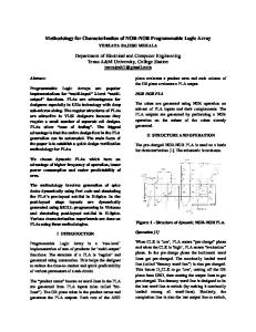
Channel Width vs. log(Circuit Size) 20 Empirical W
where λ is the pin-per-block ratio and R is the average wire-length (as, say, predicted by Feuer’s model). A fundamental assumptions of these models are that horizontal and vertical units of wire are homogeneous and uniform (i.e. all unit length, indistinguishable from each other, and with no “bias” in either direction).
15 10 5 0
A second fundamental assumption is that we have “good CAD tools”. The unreliability of this latter assumption motivates the concept of the “intrinsic” Rent parameter of a circuit as the Rent parameter arising from the best possible CAD tool [15].
6.5
7.5 8.5 log(circuit_size)
9.5
Figure 1. W vs. n for sample circuits. Brown [6,7] applied this approach to routability prediction on a simple FPGA architcture (the segmented FPGA pictured in Figure 2 which we will discuss shortly), along with a stochastic model of the probability of obtaining given switches and wires in the PLD and found a good correlation. In fact, Brown did this for several designs and also got good correlation in each case. Chan, Schlag and Zien [9] similarly applied a process of executing partitioning to calculate r, then applying Feuer and other models for wire-length and then El Gamal to predict the required W for the given circuit. Then they classify the input circuit as “easy”, “marginal” or “unroutable” for a fixed PLD architecture. Again, the authors found that they could predict whether a circuit was likely to “fit” or not. (Note that unlike ASICs which have a more continuous metric of routability, on a PLD the result reduces to “fit” or “no-fit”.) Though both of these models successfully apply the theory to estimate the required channel width for a particular design, a different design, with both a different size and different Rent parameter will have different behaviour. The interesting question from the point of view of an FPGA architect is: Can we apply this approach to a priori estimations of required interconnect for a PLD? We will address this issue in the succeeding sections. However, first let us gain perspective from some empirical data. Figure 1 shows channel width vs. log(circuit_size) for 20 MCNC [25] benchmark circuits using the VPR place and route tool [3]. It is worth keeping in mind that in some sense most of our data is really only meaningful to gain statistical significance for identification of the hard circuits, which then define our choice for the fabricated track count. (A regression equation gives a slope of 1.24 with R2 an insignificant 0.09).
2. PLD INTERCONNECT PREDICTION A PLD architecture has a fixed routing fabric, which then must be used by every input circuit. In the design of a PLD, interconnect prediction essentially means answering the following types of questions (among others): •
How many horizontal and vertical channels do I need?
•
How should wires be segmented?
•
If different wire lengths, in what ratio?
•
How can I trade off wires for switches?
•
How can I trade off delay for area (because the CAD tool can take circuitous routes if flexibility allows, but at the cost of timing).
•
How well does my device support specific common functions such as adders, multiplexors, and multiplication algorithms.
•
How will my switching be arranged? (Though this is not directly interconnect prediction, the flexibility of the switching network significantly affects line-counts.)
The word “need” is left suitably undefined, because it is not entirely clear what that means in practice. One typically thinks of this as the minimum number and distribution of wires required to fit all circuits. However, since one can easily construct pathological cases, we cannot actually guarantee 100% fitting. DeHon [11], for example, has argued that one should purposefully under-route the part because it is more efficient in terms of overall area to make parts which have a small amount of empty space --otherwise the “average” circuit would be paying for a more expensive part to benefit the abnormal circuits. In practice, we also want to be able to answer these questions with some parameters constrained. For example, inserting a new architecture family member may permit the addition of one type of wire, but not another, or growth in only one dimension, due to layout constraints. Both of the Brown and Chan studies previously mentioned target the segmented PLD architecture shown in Figure 2, which is a rough abstraction of a Xilinx 4000 [23,24] FPGA (circa 1994). This device looks very similar to a standard gate-array. The L blocks represent 4-LUT LEs which drive or feed from the wires in the channels between them via switches of the C (connection) block. The wires then also switch with each other in the S (switch) block. Using a different high-level architectural model, Altera’s FLEX 10K chips [2] are fundamentally hierarchical (See Figure 3). LEs are grouped into fully connected clusters of size 8. Clusters on the same row can drive or be driven by a horizontal wire which spans either the whole width (GH) of the chip, or half-width (HH) of the chip. Nets between different rows drive a full-length vertical wire (V) which switches onto a horizontal (GH or HH) wire before entering the cluster. To gain an appreciation for the hierarchy and the difference between these two architecture styles, one has to imagine the two architectures as significantly larger (current PLDs reach about
Page 2 of 2
P
P S
C
P
P S
C
P S
P C
P
P
P
P
P
S
P
P
P
P
P C
C
L
C
L
C
L
P p
P S
C
S
C
S
C
S
C
L
C
L
C
L
C
S
C
S
C
S
C
S
C
L
C
L
C
L
C
P P P
p
P
P
P
P
P
P S
C
P
S
P
C
P
S
P
C
P
S
P
Figure 2. Simple Segmented PLD architecture. 50,000 LEs). For 1000 LEs, the segmented architecture of Figure 2 would be an approximately 32x32 array of LEs, and the hierarchical architecture of Figure 3, 6 rows by 16 columns of clusters, each cluster containing 8 LEs. Another hierarchical architecture described by Kaptanoglu et. al [20] has its basic logic-block in arrays to a certain size (e.g. 16x16) and then tiled and connected hierarchically. Similarly, modern versions of the Xilinx segmented architecture of Figure 2 incorporated hierarchical features such as clusters and also longer lines in addition to single-length wires, significantly “bending” the uniformity rule. Hierarchical architectures introduce further problems into the prediction of interconnect requirements. El Gamal’s model assumes that tracks are segmented by uniformly single-length wires. However, in the presence of long shared lines, high usage in the bottom part of the chip could (for example) consume a large number of vertical lines in one column, causing congestion in unrelated logic on the top side of the chip. Longer lines and hierarchy motivate us to look at one of the fundamental assumptions of classical wire-length theory, namely that wires are used “optimally”.
2.1 “Efficiency” of programmable logic. When applied to ASICs, interconnect estimation has an assumption of compactness and efficiency. For example, if a point-to-point connection is of distance 3, we assume 3 units of wire will be used. This is the basis for the extension of Feuer’s model to El Gamal’s. However, programmable logic is inherently inefficient – a configurable 4-LUT makes for a very expensive AND gate, but this is the price we pay for the ability for a different circuit to use the same physical logic to implement an OR gate. Similarly, underutilization of other resources such as wires, memory, etc. allows for other designs to be implemented on the same generic device. In programmable logic, the area of the chip is dominated by switching. More specifically area can be considered as proportional to the number of configuration SRAM bits required to control the programmable switches. Thus, taking a length 10 line to go only distance 5 is not necessarily inefficient if some different circuit is able to efficiently use the length-10 wire . Though one cannot take this to the extreme and call all PLDs purely metallimited, one could consider that metal is “free” to the point where it
P
L|L L|L L|L L|L
L|L L|L L|L L|L
L|L L|L L|L L|L
L|L L|L L|L L|L
L|L L|L L|L L|L
L|L L|L L|L L|L
P P P P P
P P
P
P
P
P
P
Figure 3. Simple Hierarchical PLD Architecture. catches up with silicon area. (This, of course, is dependent on many variables.) Feuer’s region model distinguishes between length of connections “internal” and “external” to a block of logic. One can imagine extending this philosophy to predicting wire-counts within regions of a hierarchical PLD with long lines (some attempts in this direction will be discussed in Section 4, and recent work such as [10] might also be a positive step in exactly this direction), but there are no known complete treatments of the problem.
2.2 Average vs. Worst-Case Results. A second major issue with predicting interconnect in a PLD is that we have to handle the worst-case sub-circuit wherever it appears on the chip. Whereas gate-arrays can possibly distinguish between regions of the chip devoted to datapath and to control logic, PLDs must support varying degrees of datapath. Datapath has the problem of being non-average – a 32 bit bus will consume well above the average wiring resources in a particular channel. Yet putting sufficient resources in every channel for multiple busses would be inordinately expensive. Similarly, special features such as carry-chain circuitry [2,16], embedded memory blocks [18] and “alternative modes” for logic elements are not used uniformly by the user’s design, but typically need to be provided uniformly in the logic cell or cluster. It is well known that, for example, turning automatic-generation of carry chains can have a dramatic effect on fitting, both because it removes routing flexibility by introducing relative placement constraints and also because it changes the “amount” of logic in the design (in terms of LE counts) by making the logic more dense at the price of routability. Most problematic of all is that the line-count (channel width) for one chip has to support the worst-case line-count for the worst-case user netlist. Referring back to Figure 1 we can re-iterate that the behaviour of the majority of the user designs, and in particular the “average” design, is irrelevant to the architecture of the final device. This is a fundamental difference between applying interconnect theory to an algorithm as opposed to the design of hardware. In the case of algorithmic estimation, we can easily tolerate a small amount of error, and can re-tune algorithms at runtime for constant factors. However, once the architecture is fixed, a 5% error on estimating the worst-case channel interconnect could result in a significant number of designs not fitting in the part.
Page 3 of 3
2.3 Switching vs. Routing. A third fundamental difference between PLD architectures and gate arrays is the ability to trade off routing flexibility for routing itself. For example, by reducing the number of turns from V to H resources in the hierarchical part, or the population of switch blocks in the segmented part, it is possible to reduce the total area of the chip even though the number of wires per channel is increased. Brown brought this issue into his stochastic model of routability to some extent to determine “how many switches is enough”. But it would be quite interesting to get the general concept of flexibility into the interconnect usage models. As a further example of how switching has an exogenous effect on interconnect consumption, consider the case of how pins are connected into the general routing fabric. In both the models of Figure 2 and Figure 3, there is a natural correspondence between row/column and physical chip IO. Khalid [20] found for the both the XC4000 (similar to Figure 2 and FLEX8K (a predecessor to Figure 3) the pre-assignment of pins (such as would be encountered for a user who is modifying a PLD after their PCB layout is finalized) can result in a dramatic increase in both wire-count and circuit timing. A further switching-related issue is that of secondary signals. In ASICS, a small number of secondary signals (clock, reset, enable) can be routed independently, and don’t really affect other nets. In a prefabricated PLD, however, the secondary signal network already exists, and the ‘availability’ of the specific clocks or signals is often constrained within different regions, affecting how placement occurs, and hence line counts.
2.4 Uniformity. When we restrict ourselves to the uniform architecture of Figure 2, it is often possible to predict results of some interconnect issues. Betz and Rose [3,4] looked at two issues in interconnect distribution. Using at the segmented model of Figure 1(a), they considered the issue of having different channel densities in different areas of the chip. For example, should width of the center channels be larger than that of the non-center channels? (Interestingly enough, they found the answer to be no.) Also, what happens to channel density if we build a non-square PLD (e.g. 3:1)? They find that a correspondingly larger track-count is required in the direction of the longer side. One could argue qualitatively that both these results could be predicted by the classical theory. Feuer’s analysis states that for a given region of size s, the number of external connections is fixed (on average) independent of its locaion. Thus a region on the outside of the chip has the same number of connections (though half the number of directions) to go in, balancing out the number of connections. However, to quantify this relationship and reach the same conclusion as Betz’s empirical work would be difficult. No modern PLDs meet the uniformity assumptions of the classical theory. In later Virtex versions of Figure 2, LEs were grouped into clusters, a heterogeneous choice of wires (1, 2, 4, etc. and fulllength wires which pass through S without switching) was added. And the architecture of Figure 3 gained further hierarchy with the APEX architecture (discussed later in this paper).
Figure 4. Multiple heterogeneous wire-types in a recent PLD (Mercury family from Altera) Figure 4 shows a recently announced Altera device that further complicates any theory of interconnect relative to previous parts. The “Mercury” device is largely modeled on the 10K device shown in Figure 2, but adds specific new wire-types: “leap lines” to provide short vertical connections between rows, “RapidLab” interconnect, which are centered, staggered lines directly driven by individual LEs (meaning that they are faster, but less flexible). Most interesting of all is that the basic global wires come in both normal and fast or “priority” flavours – i.e. the chip has a build-in distribution of thick wires for critical connections and thin wires for normal connections. Introducing this heterogeneity not just in distribution of lengths, but distribution of flexibility introduces some fundamental issues in any theory of interconnect for the base part.
2.5 Delay vs. Area Delay and area are fundamental tradeoffs in the design of PLD architectures. The fewer switches used, the closer a PLD comes to ASIC performance. However, the cost for this better delay comes either in overall fitting or in wire area. Ahmed and Rose [1] found that an architecture based on 2 or 3 input LUTs better for area, which contrasts with earlier results [6] that LUTs of size 3 or 4 were most efficient. This points out that as geometries change the relationship between routing and switching changes, and PLD architectures are very sensitive to this. Because ASICs do not have the switching vs. wire tradeoff for either delay or area, they do not have to consider this issue. However, in the design of PLDs, it is important to know when the relationship changes. A second result in this paper was that LUTs of size 4 to 6 further clustered into groups of size 4 and 10 are superior for area and delay when taken together. The Mercury device of Figure 4 adds further complication. By having two logically identical resources with different delay properties (the normal and priority global interconnect wires) we bifurcate the interconnect prediction problem. In addition to predicting how many vertical channels we need we also need to know, across a range of designs, how many should be fast and how many should be normal speed.
Page 4 of 4
P = 0.5626B + 2 R2 = 0.7906
log P
A second issue arising in the context of delay has to do with the non-critical connections. For area reasons, an ASIC would not consider a widely circuitous route. But in a PLD, we already “paid” for these prefabricated wires. An good place and route could go to great pains to use these “free” wires inefficiently if it allows a more critical connection to have even a slightly faster path.
3. SOME EMPIRICAL DATA P = 0.7788B + 0.6973 R2 = 0.8608
Let us consider some empirically determined Rent parameters.
Figure 5 shows the data for a set of about 40 similarly sized industrial designs. (These are sorted simply by r so that the distribution is visible.) We can immediately note that we have a reasonable and uniform distribution of Rent parameters following the conventional wisdom of 0.5 < r < 0.8 with few designs outside this range. The constant 2k did vary between designs (between 1.5 and 5, with a mean of about 2). One could argue this range is a little bit higher than expected. This begs some interesting questions: Is this due to timing-driven placement? Possibly to the dominance of communications circuits in the PLD market? Is it due to the fundamental nature of PLDs, in that wire-count minimization is a means to fitting, but not the actual goal? Or would these designs give the same results in an unconstrained partition tree? How much of the result is due to the carry-chains, memories and secondary signal effects previously discussed? Since the partitioner used is based on a high-quality multi-level algorithm I do not consider the quality of the tool to be a significant issue. Figure 6 shows a detailed look at the data for a particular design (in this case a design with a relatively high r value). There are two important points to note. The first is that we can observe clumps in the data corresponding to the sampled partition boundaries of the
Unconstrained r
1 0.8 0.6 0.4 0.2 0
Figure 5. Unconstrained r for many netlists (10000 to 15000 LEs in each)
log B Figure 6. Rent plot (high r) (~10000 LE design) Unconstrained r = 0.78. Fixing k=ln(4) r = 0.56
P = 0.6522B + 1.8435 log P
To calculate an individual Rent parameter for a given design, I implemented it in the target device (for the designs of Figure 4 this was a 16,640 LE APEX20K400E as shown later in Figure 8). This device has wires organized hierarchically. The CAD flow used was a timing-driven multi-level partitioning based flow such as described in [19]. At each step of the recursive partition, the tool outputs the appropriate data-points (#LEs and #external connections) relevant for calculating the Rent parameter. I then generated a log-log OLS regression to solve for r (k was allowed to vary in order to fit the curve).
P = 0.5854B + 1.694 R2 = 0.6215 log B Figure 7. Rent plot for “many designs” Unconstrained r = 0.65. Fixing k=log(4) r = 0.65 architecture. The more important issue is the effect of fixing k. The classical literature tends to refer to k as “often the average block-degree + 1”, so I did a second regression fixing the intercept at 2 (log2(4), for 1 + an average LUT in-degree of 3). The “unconstrained” curve fit with r=0.78 drops dramatically to r=0.56 when k is constrained. So how might we apply this data to interconnect requirements for the PLD in question? (A completely separate problem is that because the part didn’t exist, most of the designs for this analysis also didn’t exist at the time the architecture was defined.) One solution might be to calculate the Rent parameter of the “superdesign” containing all the previously calculate data-points. Figure 7 shows a scatter plot and regression analysis for the set of all data points. The unconstrained regression gives r = 0.58. However this is definitely not solving our line-count problem, because it speaks to the average partition. If we want the majority of our designs to fit, we have to target some type of “upper envelope”. The second trend-line shows an ad-hoc (hand placed) line to suit this purpose. I hand-selected a line with k=4 and covering “most points” in the partition tree, and came up with a required Rent exponent of 0.65. Doing this, however, would be a major error in data analysis: As previously pointed out in the discussion of Figure 1, the vast majority of our designs are really quite easy to fit. Thus it is not a good idea to average our data so as to swamp the hard to fit designs.
Page 5 of 5
A different possibility is to throw away the data from the easy designs, and concentrate on the Rent parameter required to fit the hardest designs. Looking at Figure 5 a reasonable value to choose might be 0.78, which is approximately the 90th percentile. It is interesting to note out that about all we got from all this data is that a good initial guess would be to follow the upper end of the conventional wisdom.
r k
0.78
calc actual %diff
2 lab_ext = k * labsize^r
12
labsize
10 GH_int = labs * lab_ext
193
labs
16 GH_ext = k * (mlsize)^r
105
160 GH = GH_int + GH_ext
298
gows
13 row_v = k * (2*mlsize)^r
180
4. A SIMPLE MODEL FOR APEX WIRING.
gols
2 quad_v = rows * row_v
2339
Here we will apply some classical interconnect theory to predict the number of H and V wires required for an APEX device. Though, to some extent, this proposes a theory, our primary purpose is as illustration of the interconnect prediction problem.
quadsize 2080 double_v = k * (quadsize)^r
mlsize
total V = double_v + quad_v V per col = total_v / cols quad_h = k * (quadsize/2)^r
Consider the hierarchical “APEX” PLD device shown in Figure 8. The basic logic-element (LE) is a 4-input LUT and DFF pair. Groups of 10 LEs are grouped into a logic-array-block or LAB. Interconnect in a LAB is assumed to be complete. Groups of 16 LABs form a MegaLab, and signals within a MegaLab use horizontal wires called GH to drive the local interconnect of another LAB. Adjacent LABs interleave their local routing, and can communicate without using a GH line. The top-level routing consists of a left and right H line, connected by a bi-directional, programmable segmentation buffer. Similarly a top and bottom V. There are some number of H lines per row (2 * 13 rows total) and V lines per column (16 * 2 * 2 columns total). Because the device is hierarchical, a H or V line must drive a GH line in a given MegaLab in order to enter the MegaLab. A back of the envelope calculation is interesting. Consider the calculations in Figure 9. Using our known k=2 and r=0.78 values, we can get remarkably close to the true line-count of the part. We were within 7% on the GH lines. We will be a little over-routed in
H
HH
VV
V S
E L S A B B 0
E L S A B B 0
Mega LAB
.. . ... Mega LAB .. . Mega LAB .. . Mega LAB ...
E L S A B B 0 E L S A B B 0
E S B B 0
L A B 1 6
E L S A B B 0
L A B 1 6 L A B 16
E L S A B B 0
...
E L S A B B 0
Mega LA LAB B
E L S A B B 0
Mega LA LAB B
...
...
L Mega L A LAB A
L A B 1 6
16
16
E L S A B B 0
.. . ... Mega LAB .. . Mega LAB .. . Mega LAB ...
B 1 6
L A B 1 6 L A B 1 6 L A B 16
...
E L S A B B 0
Mega L LAB A
E L S A B B 0
L A B 1 6
.. . Mega LAB .. .
B 1 6
E L S A B B 0
Mega L LAB A
E L S A B B 0
E L S A B B 0
L A B 1 6
E L S A B B 0
E L S A B B 0
L A B 1 6 L A B 1 6
E L S A B B 0
E L S A B B 0
L A B 1 6
E L S A B B 0
E L S A B B 0
L A B 1 6
E L S A B B 0
.. . ... Mega LAB .. . Mega LAB .. . Mega LAB .. local . ... Mega LAB .. . Mega LAB .. . E L S A B B 0
B 1 6
E L S A B B 0
Mega L LAB A
.. . ... Mega LAB .. . Mega LAB .. . Mega LAB .. . ... Mega LAB .. . Mega LAB .. .
B 1 6
L A B 1 6 L A B 1 6 L A B 1 6 L A B 1 6 L A B 1 6
GH Figure 8. APEX hierarchical PLD, top-level view, showing horizontal (H), vertical (V), MegaLab-horizontal (GH) and LAB-local (local) routing lines.
double_h = k * quadsize^r total H = quad_h + double_h H per row = total_H / rows
279
6.7
775 3113 97
80 21.6
451 775 1226 94
100 -5.7
Figure 9. “Back of the envelope” wire-length calculations for H, V and GH lines on APEX400E. V, and slightly under-routed in H. But overall we are off to a pretty reasonable start. Let us ignore for now that our initial k and r came from productionquality place and route on the part itself (we also ignored all connections to the embedded RAM of each MegaLab), and look at some sensitivity analysis on our current result. Without the previous curve-fits, we probably would have chosen k=4 rather than k=2. Unfortunately, that results in 595 GH lines, 195 V lines and 189 H lines – a factor of 2 in each direction. Even modifying k to 2.2 from the original 2 increases our error to 20% in GH, 30% in V (H error dropped to 4%). Playing with r is equally problematic. A reasonable a priori guess on (k,r) might have been (4, 0.73). This results in errors between 30% and 80% on the various linecounts. It is only when we use our own data, curve-fit to the specific architecture we are defining with production quality tools that we can get close, and even then we are off by 10%. It is worth pointing out that 10% error in one direction likely results in 5-10% die bloat, while 10% error in the other direction would have dramatic negative effects on fitting.
5. CONCLUSIONS AND FUTURE WORK. There really is a lack of theoretical understanding on how to design interconnect for programmable logic. Though we can make qualitative guesses at interconnect using the classical theory, the reality is that we cannot get very close to the quality of results that we can achieve empirically. Without empirical analysis to back up the theory we we would make large mistakes in defining our architecture. Some of the reasons for this have been outlined in this paper: PLD wires are neither uniform nor continuous. The efficiency that is assumed in most theoretical models is not present in PLDs. And the premise of “average” or expected prediction is appropriate for CAD algorithms, but not for estimating the worst-case channelwidth for a range of different netlists.
Page 6 of 6
This introduces many new questions and challenges for interconnect prediction: How can we model “inefficiency” in the Rent model? In Section 4, we cheated by having an unrealistic amount of information about the partitioning hierarchy as specifically applied to our device with a large amount of data. But even with this information it would be hard to modify the model to handle relatively minor modifications such as different amounts of segmentation (e.g. 0, 4 or 8 segments). How do we effectively model the “worst case” rather than the average case. In the calculations of Section 4 we again cheated – by assuming a distribution beforehand, we chose the 90th percentile as a starting point. But without knowing the routability of our architecture beforehand this would not be possible. What about tradeoffs between switching and routing? Between delay and area? The architecture of PLDs requires these as tradeoffs, and a way to incorporate them into the model would be be quite useful.
6. ACKNOWLEDGMENTS John Valainis wrote the multi-level partitioner and necessary hooks to extract the data for Section 3. The analysis discussed in Section 4 parallels some work done by Jay Schleicher and Bruce Pedersen at Altera.
7. REFERENCES [1] E. Ahmed and J. Rose, “The Effect of LUT and Cluster Size on Deep Sub-Micron FPGA Performance and Density”, in Proc. ACM/IEEE Symp. On FPGAs (FPGA00), Feb, 2000, pp. 3-12. [2] Altera Corp. Device Data Book, 2000. [3] V. Betz, J. Rose and A. Marquardt. Architecture and CAD for Deep-Submicron FPGAs, Kluwer (Norwell, Mass), 1999. [4] V. Betz and J.S. Rose, “Effect of the Prefabricated Routing Track Distribution on FPGA Area Efficiency”, IEEE Trans. VLSI, Sept 1998, pp. 445-456. [5] B.K. Britton et. al. “Second Generation ORCA Architecture using 0.5µm Process Enhances the Speed and Usable Gate Capacity of FPGAs”, in Proc. IEEE Int. ASIC Conf., Sept 1994, pp. 474-478. [6] S.D. Brown, Routing Algorithms and Architectures for Field-Programmable Gate Arrays, Ph.D. Thesis, University of Toronto, January 1992. [7] S.D. Brown, R.J. Francis, J.S. Rose and Z.G. Vranesic. Field-Programmable Gate Arrays. Kluwer Academic Publishers, Norwell, Mass. 1992. [8] A.E. Caldwell, A.B. Kahng, S. Mantik, I.L. Markov and A. Zelikovsky, “On Wirelength Estimations for Row-Based Placement”, IEEE Trans. CAD 18(9), 1999. pp. 1265-1278. [9] P.K. Chan, M.D.F. Schlag and J.Y. Zien, “On Routability Prediction for Field-Programmable Gate Arrays”, in Proc.
30th ACM/IEEE Design Automation Conference (DAC), 1993, pp. 326-330. [10] P. Christie and D. Stroobandt, “The Interpretation and Application of Rent’s Rule”, IEEE Trans. VLSI Systems, Special Issue on System Level Interconnect Prediction, Dec 2000. [11] A. DeHon, “Balancing Interconnect and Computation in a Reconfigurable Computing Array (or, why you don’t really want 100% LUT utilization)”, in Proc. ACM/IEEE Symp. On FPGAs (FPGA98), 1998, pp. 69-75. [12] W.E. Donath. “Placement and Average Interconnection Lengths of Computer Logic.” IEEE Trans. Circuits and Systems 26(4), (April, 1979) pp 272-277. [13] A.A. El Gamal. “Two-dimensional stochastic model for interconnections in master-slice integrated circuits.” IEEE Trans. On Circuits and Systems, 28(2), (Feb 1981) pp. 127138. [14] M. Feuer. “Connectivity of Random Logic.” IEEE Trans. Computers, 31(1), (1982), pp. 29-33. [15] L. Hagen, A.B. Kahng, F.J. Kurdahi and C. Ramachandran. “On the Intrinsic Rent Parameter and Spectra-Based Partitioning Methodologies.” IEEE Trans. CAD, 13 (1994), pp 27-37. [16] S. Hauck, M. Hosler and T. Fry. “High Performance Carry Chains for FPGAs”, in Proc. ACM/IEEE Symp. On FPGAs (FPGA98), Feb, 1998, pp. 223-233. [17] W.R. Heller, W.F. Mikhail and W.E. Donath, “Prediction of Wiring Space Requirements for LSI”. Journal of Design Automation and Fault Tolerant Computing, May 1978, pp. 117-144. [18] F. Heile and A. Leaver, “Hybrid Product Term and LUTBased Architectures using Embedded Memory Blocks”, in Proc. ACM/IEEE Symp. On FPGAs (FPGA99), Feb, 1999, pp. 13-16. [19] M. Hutton, A. Leaver and K. Adibsamii. “Timing-Driven Placement for Hierarchical Programmable Logic Devices”, in Proc. ACM/IEEE Symp. On FPGAs (FPGA01), Feb, 2001, pp. 3-11. [20] M. Khalid and J. Rose. “The Effect of Fixed IO Posititioning on the Routability and Speed of FPGAs”, in Proc. Canadian Workshop on Field-Programmable Devices, 1995, pp. 474-478. [21] S. Kaptanoglu, G. Bakker, A. Kundu, I. Corneillet and B. Ting. “A New High-Density and Very Low Cost Reporogrammable FPGA Architecture”, in Proc. ACM/IEEE Symp. On FPGAs (FPGA99), Feb, 1999, pp. 3-12. [22] J. Schleicher and B. Pedersen. Personal communication. [23] S. Trimberger, K. Duong and B. Conn. “Architecture Issues and Solutions for a High-Capacity FPGA”, in Proc. ACM/IEEE Symp. On FPGAs (FPGA97). Feb, 1997, pp.3-9. [24] Xilinx Corp. The Programmable Logic Data Book, 1996. [25] S. Yang, “Logic Synthesis and Optimization Benchmarks User Guide”, Version 3.0, Microelectronics Center of North Carolina, January 1991.
Page 7 of 7