NBER WORKING PAPER SERIES

INTERNATIONAL BUSINESS CYCLE SYNCHRONIZATION IN HISTORICAL PERSPECTIVE Michael D. Bordo Thomas F. Helbling Working Paper 16103 http://www.nber.org/papers/w16103

NATIONAL BUREAU OF ECONOMIC RESEARCH 1050 Massachusetts Avenue Cambridge, MA 02138 June 2010

This is a revised version of a paper prepared for the International Symposium on Business Cycle Behaviour in Historical Perspective, University of Manchester, June 29-30, 2009. We are grateful to Matteo Ciccarelli for comments on an earlier draft of the paper and two referees for helpful suggestions. The views presented in the paper reflect only those of the authors and should not be attributed to the IMF or IMF policy. The views expressed herein are those of the authors and do not necessarily reflect the views of the National Bureau of Economic Research. © 2010 by Michael D. Bordo and Thomas F. Helbling. All rights reserved. Short sections of text, not to exceed two paragraphs, may be quoted without explicit permission provided that full credit, including © notice, is given to the source.

International Business Cycle Synchronization in Historical Perspective Michael D. Bordo and Thomas F. Helbling NBER Working Paper No. 16103 June 2010 JEL No. F0,N0 ABSTRACT In this paper, we review and attempt to explain the changes in business cycle synchronization among 16 industrial countries and the over the past century and a quarter, demarcated into four exchange rate regimes. We find that there is a secular trend towards increased synchronization for much of the twentieth century and that it occurs across diverse exchange rate regimes. This finding is in marked contrast to much of the recent literature, which has focused primarily on the evidence for the past 20 or 30 years and which has produced mixed results. We then examine the role of global shocks and shock transmission in the trend toward synchronization. Our key finding here is that global (common) shocks generally are the dominant influence.

Michael D. Bordo Department of Economics Rutgers University New Jersey Hall 75 Hamilton Street New Brunswick, NJ 08901 and NBER [email protected] Thomas F. Helbling International Monetary Fund 700 19th Street NW Washington DC 20431 [email protected]

-3-

I. INTRODUCTION The synchronized rapid and dramatic decline in output across the globe in the second half of 2008 put an abrupt end to the spreading musings of decoupling in national business cycles that emerged in early 2007 when the U.S. economy started slowing. In fact, the current global slump has been a striking reminder of how synchronized national business cycle downturns can be. This experience is in marked contrast with the experience of the two decades leading up to 2007, during which it was difficult to find strong evidence of increased or increasing business cycle linkages among industrial countries. Depending on the sample period, output correlations have even decreased in recent decades, largely on account of a remarkable cycle de-synchronization among the major industrial countries in the late 1980s and early 1990s (Helbling and Bayoumi, 2003).1

In this paper, we look at international business cycle synchronization from a historical perspective. The merit of such an approach is that short sample periods may mask important trends in synchronization patterns. In the short term, much of the business cycle dynamics depends on the shock dynamics, which tends to overshadow the effects of integration. Against this, we review and attempt to explain changes in international business cycle synchronization over 120 years using a framework in the tradition of the impulse-propagation approach to business cycles. Specifically, we seek to determine whether synchronization has increased and, if so, whether the changes in synchronization reflect changes in the nature of the impulses (the “shocks”) driving the economies, particularly the role of global shocks, changes in the 1

See also Doyle and Faust (2003) and Kose, Otrok, and Whiteman (2008).

-4-

transmission channels, or both. On the basis of this analysis, we then examine the relationship between business cycle synchronization and globalization and the role of financial factors in the dynamics of global output shocks.

From a historical perspective, the evidence in favor of increased business cycle synchronization is clear-cut. We find a secular trend towards increased synchronization that occurs across exchange rate regimes. This evidence is rather puzzling, however, considering the usual explanation for increased synchronization. While there appears to be an almost linear increase in business cycle synchronization over time, the level of globalization, that is, the degree of crossborder integration in markets for goods, capital, and labor, has followed a U-shaped pattern during the same period (Obstfeld and Taylor, 2003, and Bordo, Eichengreen and Irwin, 1999). Starting from a relatively high degree of globalization during the period of the classical gold standard, international integration decreased sharply during the interwar period before it began to rise again, first slowly during the Bretton Woods period and then more rapidly in the current floating rate period. Recent studies have documented that the degree of globalization prevailing in the 1880s was only reached again 100 years later (ibid.).

These results are not necessarily surprising from a theoretical perspective since the correlation between business cycle synchronization and integration is not necessarily positive. For example, Krugman (1993) noted that stronger trade integration may lead to greater regional specialization, which can lead to less output synchronization with industry-specific shocks. Relatedly, Heathcote and Perri (2004) showed how increased financial integration may be an endogenous

-5-

reaction to the regionalization of real sector linkages, as the latter allow for gains from the global diversification of asset portfolios.

For this investigation, we use annual data for 16 countries that cover four distinct eras with different international monetary regimes. 2 The four eras covered are 1880-1913 when much of the world adhered to the classical Gold Standard, the interwar period (1920-1938), the Bretton Woods regime of fixed but adjustable exchange rates (1948-1972), and the modern period of managed floating among the major currency areas (1973 to 2008). Across the four eras that we examine, the variation in cross-border integration in the markets for goods, capital and financial assets has been considerably larger than over the last 20 years while the influence of particular shock realizations appears arguably to have been somewhat less important. The annual data for 16 industrial countries that we use in this paper come from Mitchell (1998a, 1998b, and 1998c) and other sources. They were used by Bergman, Bordo, and Jonung (1998) and Bordo and Jonung (2001).3 Analyzing business cycle features with annual data implies that higher frequency features are not captured adequately. Nevertheless, we believe that using a much longer data sample provides a much-needed broader and complementary perspective on business cycle synchronization despite these problems. Our approach follows Bergman, Bordo and

2

These references also provide more details on the data. The countries included in our data set are Australia, Canada, Denmark, Finland, France, Germany, Italy, Japan, Netherlands, Norway, Portugal, Spain, Sweden, Switzerland, the United Kingdom, and the United States. In some of the tables, we list the countries by their geographical proximity rather than in alphabetical order. 3

The IMF’s International Financial Statistics was used to update the dataset to 2008.

-6-

Jonung (1998) and Backus and Kehoe (1992), who have shown the merit of looking at business cycle phenomena from a long-term perspective.4

The paper is organized as follows. Section II discusses conceptual issues regarding international business cycle synchronization and provides the basic stylized facts. The subsequent section looks at the role that changes in this structure of shocks may have played in the observed changes in the synchronization of cycles. Section IV considers the role of global shocks and financial factors in cycle synchronization. Section V analyzes the relationship between business cycle synchronization and the path of globalization. Section VI concludes.

II. CROSS-COUNTRY BUSINESS CYCLE SYNCHRONIZATION OVER TIME The notion of business cycles becoming increasingly synchronized across countries captures the observation that the timing and magnitudes of major changes in economic activity appear increasingly similar. For example, in the current slump, output collapsed in all major economies at about the same time. Despite frequent use, however, definitions of synchronization vary widely in the literature, As noted by Harding and Pagan (2004), most definitions are not capturing business cycle synchronization in the tradition of the National Bureau of Economic Research (NBER) because they are based on other business cycle concepts. In their paper, they develop a statistical apparatus that allows for measurement and testing of cycle synchronization in the NBER tradition. Specifically, they consider national business cycles to be synchronized if

4

Unlike these papers, we focus on international synchronization and devote less attention to the comparison of national business cycle properties such as output volatility or output-consumption comovements.

-7-

turning points in the corresponding reference cycles occur roughly at the same points in time. On this basis, they have derived a statistical measure, the concordance correlation, that allows one to test whether national cycles are significantly synchronized or not. This approach to measuring synchronization boils down to national business cycles being in the same phase—expansions and recessions—at about the same time.

In this paper, we will not follow Harding and Pagan. Analyzing cycles using turning points would add an unwarranted layer of complexity to the analysis. Ultimately, as Harding and Pagan (op. cit.) have shown, their measure of cycle synchronization depends on the moments of output growth. For an analytical understanding of the changes in the synchronization, it is, therefore, sufficient to focus on the changes in these moments.5 Hence, to establish the stylized facts, we can use correlations among output growth rates as a measure of the strength of cross-country linkages in macroeconomic fluctuations. This is also the most widely used measure in the recent academic literature on the international business cycle.

We will, however, follow Harding and Pagan (2003, 2004), Stock and Watson (1999), and others by using real gross domestic product—or output in short—as the measure of aggregate economic activity or the business cycle rather than synthetic reference cycle series based on a number of series (the NBER approach).

5

In Bordo and Helbling (2004), measurement issues are discussed in greater depth, and patterns of cycle synchronization are established using three different measures.

-8-

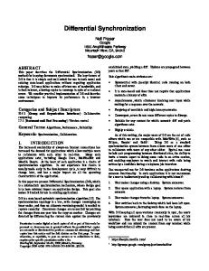
Figure 1 shows the correlation coefficients for log output growth by percentile for the four eras. The distribution of the correlation coefficients differs substantially from era to era. In particular, there has been a tendency toward higher, positive output correlations, not just a one-time level increase in synchronization. During the Gold Standard, about one half of all country pairs were characterized by negative output correlations and the average output correlation coefficient is about 0 (Table 1). A first important step toward synchronization occurred during the interwar period, when the share of negative correlations fell below 30 percent while the average correlation increased to about 0.15. A subsequent reversal during the Bretton Woods era was small, and correlations remained, on average, above those found for the Gold Standard era. A second important increase then occurred during 1973-2008, when less than 10 percent of all correlations were negative and the average correlation was 0.33.

Many of these changes in correlations across eras are statistically different from zero, on the basis of both nonparametric and parametric tests.6 The issue of statistical significance is relevant since the confidence intervals for the bilateral correlation coefficients are relatively wide given the relatively few observations per era.7

The non-parametric Wilcoxon Rank Sum test is a test of the null hypothesis that the location of the bilateral correlation coefficients (the elements of the population) is identical across eras. As 6 7

See Bordo and Helbling (2003) for more details.

The sampling standard deviation of estimated correlation coefficients depends on the size of the estimated coefficient and the number of observations. Given the former, small samples tend to amplify the sampling uncertainty greatly. For example, for a correlation coefficient of 0.15—the average for the interwar period—the standard deviation for a sample of 20 observations is 0.23. With 50 and 100 sample observations, the standard deviations decline to 0.14 and 0.10, respectively.

-9-

shown in Table 2, the test results suggest that the upward shifts in the distribution of the correlation coefficients are significant at the 5 percent level for the interwar period (compared to the Gold Standard era) and for the modern floating era (compared to both the interwar and the Bretton Woods eras). However, the downward shift in the distribution of correlations from the interwar to the Bretton Woods eras is not significant.

Parametric tests of the null hypothesis that two correlation matrices are equal, based on the approach proposed by Jennrich (1970), suggest rejection of the hypothesis that output correlations in the modern floating era have been equal to those recorded in earlier eras (Table 2). The marked increases in the correlations in the floating era are thus statistically significant. Among the other eras, however, the null hypothesis of equality between of correlation matrices is accepted. Overall, these tests support our view that, from a historical perspective, there is strong evidence of an increase in business cycle synchronization.

So far, we have looked at business cycle synchronization through a global lens, noting the increased synchronization without consideration for other factors. However, one would expect that synchronization patterns differ considerably across groups of countries, depending on factors such as “gravity” or country size. The evidence clearly illustrates that the extent to which gravity has shaped the synchronization trends depends on the region (see the results in Table 1). For core European countries (the old “EEC”) and Continental European countries, the increase in business cycle synchronization was clearly much sharper than the general increase. At the other end of gravitas, business cycle synchronization between Japan and the other countries in the panel has

- 10 -

increased by less. In particular, there is no evidence for an increase between the Bretton Woods era and the modern floating rate period.

The fact that the increase for all Continental European countries was smaller than that for the Core European countries suggests that the forces of gravity are affected by common policies, preferential trading agreements, and specific currency arrangements. The increase in correlations among the Anglo-Saxon countries is also remarkable even though it seems more difficult to attribute this to forces of gravity.8 While we do not believe that common institutions and heritage among the Anglo-Saxon countries account directly for the increased synchronization, as Otto et al. (2001) have argued, they likely have fostered similar patterns in the transmission of shocks through what appear to be similar, market-based financial systems.

While the regional perspective reinforces the notion of a trend increase, it should be noted that stark regional differences have only really emerged during the modern floating rate period. Forces of gravity were not a factor behind business cycle synchronization during the classical Gold Standard, as differences in correlations among regions were minor, with the high correlation between Canada and the United States and, to a much lesser extent, among the Scandinavian countries, being the main exceptions. During the Bretton Woods period, increased regional synchronization began to emerge in the core European countries. Interestingly, the increased synchronization during the interwar period was primarily on account of an increased

8

The emergence of strong business cycle linkages among core European countries and among the Anglo-Saxon countries was noted, among others, by Helbling and Bayoumi (2003) and Stock and Watson (2005).

- 11 -

synchronization between the cycles in the United States and other countries, which in turn seems to reflect the equity boom bust cycle and its effects from the mid-1920s to the mid-1930s.

The experience with synchronized recessions over the past few decades seems to suggest that downturns tend to be more common than expansions. The historical record shows that greater output synchronization during downturns is a phenomenon that has emerged with the tendency toward greater business cycle synchronization more generally. In the gold standard era, the average correlation coefficient for output growth between two countries when at least one of them was in recession was only marginally higher than that based on observations for the entire era (lower panel of Table 1).9 Over time, however, output correlations during recessions have risen even faster than they have when measured for entire eras. Increased business cycle synchronization over time, therefore, does not seem driven by the frequency of recessions. In fact, the average number of countries in recession per year has varied across the four eras without trend. Starting from 4 during the gold standard era, the number increased to 4.8 during the interwar period, then fell to less than 1 in the Bretton Woods periods, and finally rose to about 1.7 in the modern floating rate era.

We also examined whether there were large changes in the magnitudes of correlation coefficients over the modern floating era, given some recent studies suggesting that there had been a decrease in output synchronization over the past two decades after 1985 than an increase (e.g., Heathcote and Perri, 2004). Specifically, we compared output correlations over 1986-2006 with those for 9

Following the NBER approach, recession periods were identified as those years in which log output growth was negative.

- 12 -

the entire modern floating era which spans the period 1973-2008. The last column in Table 1 shows that the differences in correlations coefficients are very small. Given the number of observations, these differences are not statistically significant. We conclude from this exercise that the secular trend toward increased business synchronization seems to be a robust result.

So far, all the cycle correlations we have studied were based on log first differences of output. Does the detrending method matter for our findings? Naturally, high frequency noise is not a great concern, given our panels of annual data, but it is possible that the increases in cycle correlations from the 19th to the end of the 20th century really reflect changes in trend comovements. In Bordo and Helbling (2004), we also examined correlation patterns in bandpassfiltered log output data. The results show that the detrending method makes little difference and that the same principal changes in the patterns of cycle synchronization are found with bandpassfiltered output data.

III. EXPLAINING SYNCHRONIZATION: THE ROLE OF SHOCKS AND TRANSMISSION Using a standard measure of business cycle synchronization, we found evidence of increased cross-country business cycle synchronization over time among industrial countries. From an impulse-propagation perspective, the increased synchronization could reflect changes in the nature of the impulses (the “shocks”) driving the economies, especially changes in their crosscountry correlations, changes in the transmission channels and mechanisms, resulting inter alia from increased integration, or, most likely, both.

- 13 -

Disentangling the relative contributions of the changes in the correlation of shocks and changes in the transmission channels to the changes in output correlations is difficult, however, as this would require a comprehensive structural model of the economy that can be estimated empirically. Such a model, which would need to allow for factors such as changes in trade and financial integration and a multitude of shocks, seems beyond our reach, given the current state of the art in multi-country modeling. Financial integration, for example, is not yet satisfactorily accounted for in any of the leading multi-country models.

Against this background, we will proceed with a more modest research agenda. In this section, we will focus on deriving measures of the impulses driving each economy and study the changes in their variance-covariance structure. On this basis, we will then attempt to assess the extent to which changes in this structure of shocks may help to explain the observed changes in the synchronization of cycles.

A. Analytical Framework To structure our discussion, we follow Canova and Dellas (1993) and use the following canonical, simple model of joint output dynamics in a two-country set up:10

 y1t   a11    y2 t   a21 10

a12   y1t 1    1t     a22   y2 t 1   2 t 

(3.1)

Canova and Dellas (1993) show how a very stylized two-country real business cycle model implies such a bivariate vector autoregressive representation. Doyle and Faust (2002) use a simple error-components structure to illustrate similar issues.

- 14 -

where yit denotes the log output growth rate in country i. Following Stock and Watson (2005), the error vector ν is assumed to be determined by the following factor structure:11

 1t   1t     G t     2t   2 t 

(3.2)

In this factor model of the VAR errors, ζ is a global shock and ηi is a country-specific idiosyncratic shock. G is a vector of factor loadings. The matrix moving average representation of the factor VAR (FAVAR) model follows as: Yt  C ( L)G t  C ( L)t ,

(3.1)

The unconditional variance-covariance matrix of the vector yt is given by: E[YtYt ]  C (1)G  G C (1)  C (1) C (1)

(3.2)

provided that independence between the global factor ζt and the idiosyncratic errors ηit holds.

What can explain increased output synchronization—as measured by the correlation between outputs of countries 1 and 2—in this model? General statements are difficult to make since determination of signs and magnitudes of the partial derivatives of (3.2) depend on multiplicative terms of the underlying parameters. However, partial derivatives around parameter values that

11

In contrast, in the standard dynamic factor model, the coefficient matrix A is usually assumed to be zero and the dynamics arise from the factors, which are modelled as autoregressive processes.

- 15 -

are empirically relevant, notably positive first-order autocorrelation coefficients, a11 and a22, and positive spillover coefficients, a11 and a22, suggest three reasons for increased output synchronization:12 

Increases in the variance of the global shock relative to the country specific idiosyncratic shocks.



Increases in the size of the “transmission” coefficients a12 and a21, which determine the spillover effects that shocks in country 1 have on country 2 and vice versa as well as those arising from the effects of global shocks elsewhere.13



Increases in the size of the “autoregressive” coefficients a11 and a22, as greater persistence in a country’s output fluctuation increases the scope for spillovers. Compared to the previous two factors, the effect of changes in the autoregressive coefficients on output correlations tends to be small.

Extending the model to our 16-country panel leads to the following equation for a country i: yi ,t     i yi ,t 1 

16



j 1, j  i

 ij y j ,t 1   i ,t

(3.3)

and

 t  G t   t

(3.4)

12

The reader should also recall that the idiosyncratic shocks are not correlated by assumption in thes two country framework. Otherwise, the global shock could not be identified. With a larger cross-country dimension, however, limited correlation among idiosyncratic shocks becomes possible, as discussed below. 13

In the simple model of Canova and Dellas (op. cit.), these coefficients follow from the production structure, as foreign intermediate goods are needed to produce the final consumption goods.

- 16 -

where the vector Nt includes all errors νit and the vector Ht all idiosyncratic shocks ηit (i=1,…, 16). Estimating this general FAVAR model in our sample is difficult. Given few observations for each era, very few degrees of freedom would be left if the model were estimated even with one lag. For the interwar era, the number of common observations for all 16 countries is even less than the number of parameters, so that comparability of the model across eras could not be ensured. In the circumstances, we imposed a priori restrictions and estimated two more restricted versions of the general factor VAR model for each era.



The center country model. In this version, the equation for each country’s real GDP growth includes lagged own GDP growth and lagged GDP growth in the center country (the United Kingdom in the Gold Standard era and the United States in the other eras). In other words, the coefficients δij are assumed to be zero for all j except for the center country. The rationale behind this model is that idiosyncratic shocks in the center country can be transmitted through the traditional channels while idiosyncratic shocks elsewhere have only limited effects on other countries.



The trade linkages model. In this version, the equation for each country’s real GDP growth includes lagged GDP growth and lagged GDP growth in important trading partner countries (the ones reported in Mitchell, 1998a, 1998b, and 1998c).14 The rationale behind this model is, of course, straightforward.

14

Mitchell (op. cit.) reports bilateral trade with 5 to 7 important trading partners for the Gold Standard and the Interwar eras. We used those with entities in our data set only.

- 17 -

We estimated the models with a two-step, semi-parametric procedure, similar to the one used by Bernanke et al. (2005), for estimating our two factor vector-autoregressive model. In the first step, we used SURE estimators to obtain the coefficients βi and δij and the residual series νit. In a second step, we used the nonparametric static approximate factor model of Ng and Bai (2002) to obtain the global shock ζ and the idiosyncratic shocks ηi from the residual series νit. This model allows for serial correlation, heteroskedasticity and limited contemporaneous cross-correlation in the idiosyncratic components. Following standard practice in the literature, we use the first common factor to measure the common shock driving cross-country business cycle fluctuations.15 Both models turned out to be roughly similar in terms of information criteria for all eras, although the restrictions implied by the center model compared to the trade model were rejected by standard likelihood ratio tests.

B. Results

Figure 2 summarizes the estimated coefficients in the two models.16 Two features stand out. First, the average autoregressive parameter (i.e., the coefficient βi) across countries has clearly increased over time. For both models, the average autoregressive parameter was slightly negative during the Gold Standard era and positive during the other eras. The minimum, as indicated by the lower bound, given by the 5 percent percentile, increased over time while the maximum only

15

Bai and Ng (2002) proposed to use information criteria to determine the appropriate number of factors. However, their Monte Carlo simulations show that for panel datasets where the cross-sectional and time dimensions are as low as in ours, the tests are not very reliable and tend to imply too high a number of factors.

16

The coefficient estimates for the trade model for the interwar period implied unstable dynamics, and we do not report results for this period for this model.

- 18 -

increased in the case of the trade model.17 Second, the transmission coefficients have changed surprisingly little. For the center model, there is some evidence that the average transmission coefficient has increased slightly but the range given the 95 percent confidence interval appears to have changed only marginally. In contrast, for the trade model, the average hardly changed but the range, especially in the positive domain, increased.

We now turn to the shocks. Table 3 shows the average standard deviations of the national output series (log growth rates) and compares them with the estimated variances of the global shock and the average idiosyncratic shock.18 The standard deviations of both global and idiosyncratic shocks generally decline over time, as it was to be expected, given the decline in output growth volatility.19 However, as noted earlier, what matters for the changes in output correlations is the relative change in the standard deviations of the two types of shocks. While idiosyncratic shocks were clearly more volatile than global shocks during the Gold Standard, their volatility has, on average, declined a bit more rapidly than that of the global shock, although after the interwar period, the differences in the relative decline became small.

17

Following the stability analysis for the bilateral output correlations discussed in the previous section, we also examined parameter stability in the modern floating era. Specifically, we tested for the stability of the autoregressive coefficients, which tend to be sensitive to structural breaks in the data. Likelihood ratio tests comparing specifications of both kinds of FAVAR models with and without a structural break in the autoregressive parameters after 1985 suggest acceptance of the null hypothesis that there is no structural break. For the center model, the likelihood ratio test statistics is 20.55, while for the trade model, it is 8.752 (the 5 percent marginal significance value for χ2(16) is 26.3).

18

Naturally, only the product Gζt is identified in this factor model. We normalized the square of the factor loadings, i.e., G’G/16=1, to identify ζt. We believe this to be the natural normalization, as it allows for comparable variances between outputs and factors. The alternative would have been be to normalize the factor variance to 1 (Bai and Ng, 2002) and to let the factor loadings adjust to replicate output variances 19

The general moderation in the amplitude of output fluctuations has been analyzed by Blanchard and Simon (2001).

- 19 -

To examine the combined effects of the changes in parameters and shock properties over time on business cycle synchronization, we performed two sets of calculations. First, we performed standard forecast error variance decompositions. Table 4 presents 1 to 4-year ahead forecast error variance decompositions of the output growth rates, averaged across countries, for the four eras, distinguishing between the shares of total output variance explained by the global shock, the idiosyncratic shocks, and transmission. Specifically, the variance decomposition for output growth in country i was derived as: h

h

Et  h [ yi2,t  h ]   2  C ii2 ( s )   2  s 1

16



s 1 j 1,i  j

h   C ij2 ( s )   Ci ( s ) Ci ( s )

(3.5)

s 1

where C ii ( s ) and C ij ( s ) are elements of the matrix product C(s)G, with C and G defined earlier, and where Ci ( s ) denotes row i of the matrix C for i=1,...,16. . The first term in this equation reflects the immediate impact of global shocks on domestic output. In Table 4, it is reported under the column “Global factor-Own.” The second term captures the transmission of the effects of the global shock on other countries. The third term is the combined contribution of the idiosyncratic shocks, encompassing both direct effects and transmission. Given our approximate factor model formulation for the idiosyncratic errors, the direct effects are of two kinds, namely the purely country-specific part of the shocks and those arising from the cross-correlation among the idiosyncratic shocks. In the absence of a structural model, we distinguished the two effects by first calculating the effects of the conditional idiosyncratic shocks, that is, the effects of the shocks ηi given the idiosyncratic shocks ηj, (j=1,…16, j≠i), elsewhere, which we then subtracted from the total effects of idiosyncratic shocks to obtain the effects due to transmission and

- 20 -

idiosyncratic shock correlation.20 Denoting the variance of the conditional shocks with 2i , the column “Idiosyncratic factors-own” in Table 4 reflects the direct impact of the purely countryh

specific part of each country’s idiosyncratic shocks given by 2i  Cii2 ( s ) . This decomposition s 1

does not imply causality in the sense of the shocks ηj, (j=1,…,16, j≠i) being exogenous from the perspective of country i. On the contrary, the causality may well run from country i to the other countries. The conditional variance simply captures the part of the idiosyncratic shock variance that is uncorrelated to idiosyncratic shocks elsewhere.

The variance decomposition suggests the following. In general, idiosyncratic shocks have become less important over time in shaping each country’s output dynamics while global shocks have become more important. At the same time, the transmission of shocks across borders has also increased. Within this broad picture, however, the relative importance of these two factors in explaining the changes in the forecast error variance depends on the model and the eras used in the comparison. The results for the center model suggest that the increases in the relative variance of the global shocks account for most of the increase in output variance explained by the global factor, which itself depends on both the shock variance and transmission. On the other hand, the trade model suggests that both increases in the relative variance of the global shocks and the transmission account for the reduction in the variance share of idiosyncratic shocks. Interestingly, the increased importance of the transmission of shocks in explaining output

20

For example, the conditional distribution for the first country in the vector yi was calculated as:

     12  221 21 where the matrices 12 ,  22 , and  21 are the relevant partitions of the matrix ˆ  . 1

1

- 21 -

synchronization that the trade model indicates stems primarily from the increased transmission of idiosyncratic shocks. This suggests that it is not transmission from the center country, a channel that operates in both models, that accounts for the increased variance share of transmission. It is rather the intra-European or the intra-Anglo-Saxon country transmission that matters with regard to transmission, a fact that seems consistent with the above average output synchronization among European countries reported in Table 1. At the global level, on the other hand, it is primarily the global shocks that matter.

Next, we computed the full variance-covariance matrix of the 4-year ahead forecast errors and analyzed the changes in the average correlation among the errors. Table 5 shows the changes in average forecast error correlations over time implied by our two estimated models. It shows both the overall change and the change implied by the change in one group of parameters only (with the sum across all parameter groups being equal to a first-order approximation of the change). Regarding the latter, we distinguish between global shocks and loadings, idiosyncratic shocks and their correlation, and the VAR coefficients.21 Overall, the implied changes in forecast error correlations are remarkably close to the actual changes in average output correlations, particularly for the center model. The implications differ between models. The calculations for

21

Specifically, the first-order contribution of the changes in the global shock variance and the factor loading between the Gold Standard era, denoted with GS, and the interwar era, denoted with IW, was calculated as: 4

 s 1

C GS ( s)G IW IW G IW C ( s)  C GS ( s)IW C GS ( s)

4

 C GS ( s )G GS GS G GS C ( s )  C GS ( s )IW C GS ( s) s 1

- 22 -

the center model suggest that, on average, the increased business cycle synchronization over the four eras primarily reflects the increased importance of global shocks. On the other hand, the trade model suggests that while global shocks have become more important, the increased transmission accounts for a larger share of changes attributable to one parameter group. Between the Bretton Woods era and the modern floating era, both models indicate that increases in transmission have been relatively more important than they were between previous eras.

C. Sensitivity Analysis

Our results imply that the answer to the question about whether the observed changes in business cycle synchronization can be explained mostly with changes in impulses or transmission depends on the model. Given obvious limitations to the power of any test with our dataset, we now turn to sensitivity analysis to examine the robustness of our findings. Given the problems with short data samples, there is no scope for sensitivity analysis for the VAR parts of the models and we will focus entirely on the factor structure of the VAR residuals.

A first issue concerns the number of common factors. In line with standards in the literature, we only used the first common factor as a measure for the common shocks. As shown in Table 6, this factor always explains more than 20 percent of the residual variation. Nevertheless, the next two to three common factors also explain more than 10 percent of the residual variation. In the absence of clear benchmarks and tests, it is not clear what cut-off points should be chosen for the share of the residual variation explained by important common factors. It has been suggested in the literature to use common significance levels (Forni and others, 2000) even though we think

- 23 -

that in a sample like ours, a 20 percent cut-off is a more reasonable minimum for a common factor. However, as the results in Table 6 show, selecting a 10 percent rather than a 20 percent cut-off criterion would primarily change the relative shares of global and idiosyncratic shocks in explaining the residual variance but not the changes over time. Moreover, what has increased over time is primarily the share of the residual variation explained by the first common factor. The changes in the share of the variation explained by the second to fourth common factors are minor. This suggests that our results are quite robust with regard to the changes in business cycle synchronization on account of changes in the properties of shocks.

A second issue concerns the specification and estimation of the factor model. We used the nonparametric estimator proposed by Stock and Watson (2002), which is an asymptotic estimator insofar as it relies on a large cross-sectional dimension for the identification of the factors. Our cross-country dimension is clearly small, and the estimated common shocks may include noise from idiosyncratic shocks. We therefore also estimated a parametric version of the factor model (3.4) using a maximum likelihood procedure. For the identification of the shocks, we impose the standard restrictions in static parametric factor models. In particular, we assumed that there is one global shock with variance 1 and that the variance-covariance matrix of the idiosyncratic shocks, Ση, is a diagonal matrix. Table 7 shows the implications for the shock variances.22 In general, the estimated variances are very similar to those obtained with the nonparametric estimator for the interwar and postwar periods. They are quite different for the gold standard era for the trade model (but not the center model). The variance of global shocks 22

The average global shock variance is computed as (1/16)G’G, which is equivalent to the computations underlying the results shown in Table 4.

- 24 -

now exceeds the average of idiosyncratic shocks. Table 8 shows the implications for the implied correlations among the 4-step ahead forecast errors.

IV. BUSINESS CYCLE SYNCHRONIZATION, GLOBAL SHOCKS, AND FINANCIAL FACTORS

For a better understanding of the role of global shocks in international business cycle synchronization, Figure 3 is instructive. Each panel shows the global shocks from the trade model (solid lines) for an era, supplemented by dotted lines depicting the global shocks from a simple static approximate factor model for output growth rates (taken from Bordo and Helbling, 2004) and bars showing time dummies—the equivalent of global shocks—from an error components model that are significant at the 5 percent level.23 We estimated the latter to obtain another measure for large and important shocks. The global shocks implied by the two factorbased approaches—the trade model and the simple factor model—are surprisingly similar except for the interwar period, although the shocks from the trade model are generally smaller in magnitude. The latter finding is not that surprising since the possibility of transmission implies lower shock variances with equal output variances. The general picture emerging from Figure 3 is that global shocks appear noticeably important at times of world-wide downturns, suggesting an asymmetry between downturns and upturns.24

23

We estimated the following traditional error component model with our panel dataset:

y

i ,t

 

t

 

i ,t

where λt denotes a time dummy taking on the value 1 in time t and ηi,t a shock

specific to country i. 24

This corroborates Helbling and Bayoumi (2003), who found a similar result for the G-7 countries during 19732001 using quarterly data and a dynamic factor model to isolate common cycles.

- 25 -

The current global slump has once again illustrated the pivotal role of financial factors in international business cycle synchronization. To analyze the role of financial factors in global shocks to output growth, we have sought to relate the global shocks ζt to measures of global financial conditions. Following English et al. (2005), we constructed a global financial conditions index based on the first principal component of a cross-section of financial indicators.25 However, unlike English et al. (op. cit.), the cross-section is not a set of indicators within a country, but across the countries in our data set. Hence, our index captures common factors in national financial conditions.26

Unfortunately, the lack of a large cross-section of relevant and comparable financial variables across countries and time has forced us to consider a relatively limited set of variables only. Specifically, we constructed two such global financial conditions indices. The first one is based on real money growth in 11 countries.27 The underlying approach is not one of “global monetarism.” Instead, real money growth is considered to be a proxy variable for general credit conditions. The second index is also based on the real money growth rates for the 11 countries, but it also includes measures of real stock return for 5 countries28, real ex post short-term interest rates in 4 countries,29 and yield spreads in 4 countries.30

25

See also Swiston (2008).

26

The first principal component was derived from the residuals of AR(1) regressions of the underlying financial variables.

27

The countries are Australia, Canada, France, Germany, Italy, Japan, Spain, Sweden, Switzerland, the United Kingdom, and the United States.

28

France, Germany, Switzerland, the United Kingdom, and the United States.

29

France, Germany, the United Kingdom, and the United States.

- 26 -

As shown in Table 9, correlations between the global output shocks ζt and the two global financial condition indices generally are not significant.31 However, the charts in Figures 4 and 5 suggest that financial conditions have been important in some business cycle downturns. Time effects in our cross-section of financial variables were typically significant at times when time effects in our cross-section of GDP data were also significant. As noted earlier, “global” output shocks seem more prevalent during downturns than during upswings.

The phenomenon that there appears to be no noticeable correlation between financial disturbances and reference cycles except occasionally during broader international downturns has been noted, among others, by Morgenstern (1959, p. 64). Nevertheless, in view of the limited set of financial variables used to derive common financial disturbances, our results are preliminary at this point. Further research is needed to establish their robustness.

V. BUSINESS CYCLE SYNCHRONIZATION AND GLOBALIZATION

Overall, our results are broadly consistent with globalization. With increased economic and financial interdependence through trade and financial linkages, the scope for global shocks or the rapid transmission of shocks in the center countries has clearly increased. In addition, with global shocks, floating exchange rates do not provide much scope for insulation, since shocks affect all countries in similar ways. At the same time, business cycle amplitudes have clearly moderated 30 31

France, Germany, the United Kingdom, and the United States.

This conclusion is robust to various small modifications of the modeling assumptions. In particular, if the global financial conditions indices are based on residuals from AR(1) regressions that also include lagged GDP growth rates as regressors, the results are virtually the same.

- 27 -

during the post-World War II period, reflecting, among other factors, changes in sectoral structure, automatic stabilizers, the use of lender of last resort operations, and the use of discretionary counter-cyclical policies.32 In this context, it is interesting to note that the volatility of idiosyncratic shocks has decreased more than that of global shocks. Among other factors, this finding is consistent with the notion that the changes in the sectoral structure and the use of automatic stabilizers as well as other counter-cyclical policies have been fairly similar across the industrial countries.

Nevertheless, some aspects of our results remain puzzling. The much larger standard deviations of idiosyncratic shocks during the gold standard may be explained by structural factors, the conduct of macroeconomic policies, and measurement errors. Clearly, agriculture was much more important, rendering economies more susceptible to idiosyncratic shocks as weather conditions. Similarly, the general absence of lender of last resort policies (except mainly in the core countries) and macroeconomic stabilization policies could also have contributed to relatively larger idiosyncratic shocks. However, the fact that the transmission of idiosyncratic shocks played such little role during the classical gold standard remains puzzling for explanations that rely on globalization as the key driving force behind changes in the factors driving business synchronization.

In particular, the level of globalization, that is, the degree of cross-border integration in markets for goods, capital, and labor, has followed a U-shaped pattern during the same period (see Bordo, 32

See McConnell and Perez-Quiros (2000), Blanchard and Simon (2001), IMF (2002), and Stock and Watson (2005) for recent studies examining the volatility of output fluctuations in industrial countries, especially the United States.

- 28 -

Eichengreen, and Irwin, 1999, and Obstfeld and Taylor, 2004). . In contrast, the time path of business cycle synchronization has followed a secular increase over time, almost linear if there were not the interwar period hump. How can we explain this disconnect? Specifically, we will use the results to explore three hypotheses explaining aspects of the disconnect. First, we explore what we call the global shock hypothesis. According to this hypothesis, the above-trend degree of business cycle synchronization during the interwar period—when integration was lower than during the classical gold standard— is the result of an exceptionally large adverse global shock. Given that the interwar period was short, with the data only covering the period 1925-38, this outlier colors the sample statistics of what was really a transitional period. We found some evidence in favor of this hypothesis. According to both the center country and the trade linkages models of international business cycle dynamics, the variance of the global shock increased relative to the idiosyncratic shocks during the interwar period. Everything else being equal, this explains increased cross-border output comovements. However, the variance decomposition of the same models suggests that increased transmission accounted for most of the increased role of external factors in the determination of output variances. This suggests that despite the on-going disintegration during the interwar period, the forces of transmission can still be large. Clearly, the transmission of large shocks in the largest country, the U.S., was, unsurprisingly, a key factor in the worldwide Great Depression.

A second hypothesis is what we call the idiosyncratic shock hypothesis. This hypothesis postulates that changes in economic structure—especially the declining share of the agricultural sector in total output and the systematic use of stabilization policies—resulted in a decline in the

- 29 -

size of idiosyncratic shocks relative to global shocks. Everything else being equal, this can contribute to explaining increased cross-border output comovements. We found evidence in favor of this hypothesis for the transition from the classical gold standard to the other eras during which relative shock variances decreased. For other transitions, the changes in relative variances were, on average, very minor.

A third hypothesis postulates that while seemingly similar, the depth and breadth of cross-border integration before World War I was different from that in the current era. The two eras of globalization may thus have been more different than it is sometimes assumed. Bordo, Eichengreen, and Irwin (1999), for example, argued that global capital market integration today is broader and deeper, including a larger set of financial instruments, a larger number of more diverse financial intermediaries operating on a global scale, and a wider range of sectors using international markets for financial purposes. In addition, there has been a shift from debt to equity finance at the global level. Similarly, in international trade, the depth or cross-border integration has increased (e.g., Krugman, 1995). The share of trade in tradables production has increased with intra-industry trade and the shift toward trade in manufacturing products, and producers have been able to break production geographically at a much larger scale (“vertical production linkages”). While we intend to investigate this hypothesis more systematically, we have been constrained by a lack of data. In particular, we believe that with deeper and broader increased economic and financial interdependence through trade and financial linkages, the scope for global shocks has clearly increased and even industry-specific shocks can have global repercussions with production linkages. In addition, with highly integrated capital markets, it

- 30 -

may be in practice quite difficult to distinguish between true global shocks and what appear to be global shocks but are really rapidly transmitted shocks in the center countries.

VI. SUMMARY AND CONCLUSIONS

In this paper, we have documented that there is a secular trend towards increased synchronization for much of the twentieth century and that it occurs across diverse exchange rate regimes. This finding is of interest because it is in marked contrast to much of the recent literature, which has focused primarily on the evidence for the past 20 or 30 years and which has produced mixed results.

We then considered a number of possible explanations for the observed pattern of increased synchronization. We first ascertained the role of shocks demarcated into country-specific (idiosyncratic) and global (common). Our key finding here is that global (common) shocks generally are the main influence across all regimes and models. We note, however, that with reduced form models of the kind used in this paper, it remains difficult to distinguish between “true” global shocks and major shocks in the center country(ies). Nevertheless, financial factors often seem to be present at times when large global output shocks can be identified.

This finding coupled with earlier evidence produced by ourselves and others that business cycles since World War II have become less volatile, less frequent and asymmetric with a tendency towards recoveries exceeding downturns in duration, has some interesting implications. We suggest that what may be occurring is that the weakening in national business cycles since

- 31 -

World War II coupled with the diminution of idiosyncratic shocks reflect the forces discussed by Zarnowitz (1992) and others, such as changes in the composition of output, the advent of automatic stabilizers, improvements in discretionary monetary and fiscal policy, the implementation of effective lenders of last resort and a financial safety net, and the proliferation of private risk sharing instruments.33

At the same time, the increasing importance of global shocks and, to some extent, transmission, we posit reflects the forces of globalization, especially the integration of goods and services through international trade (Findlay and O’Rourke 2003) and the integration of financial markets (Obstfeld and Taylor 2003). Elsewhere, we have presented evidence showing a modest role for increasing bilateral trade in explaining synchronization, with stronger evidence for regional integration in Europe and North America (Bordo and Helbling, 2004). Evidence for the role of financial integration proxied by the removal of capital controls is inconclusive.

We also did some exploratory work on the role of the policy regime in explaining the pattern of synchronization. We found little evidence for the prediction that adhering to fixed exchange rates fosters synchronization except in the period since 1973, and these results appear driven largely by the process of European Monetary Union. Clearly, further research is needed.

33

We would like to emphasize that the decrease in idiosyncratic shock volatility does not necessarily imply that it is the volatility of the underlying “deep structural” shocks (e.g., a widespread drought) that we are measuring. Given that we derive the shocks on the basis of GDP series alone, it means that the effects of these deep shocks on output have diminished. There is, however, some evidence that shocks that are widely perceived as being exogenous may have an endogenous component. Barsky and Kilian (2001), for example, argue that the sharp increase in real oil prices in the 1970s was in part a reaction to the earlier massive expansion of the world money supply.

- 32 -

References

Backus, D. K., and P. J. Kehoe (1992). ‘International Evidence of the Historical Properties of Business Cycles’, American Economic Review, Vol. 82, pp. 864–88. Bai, J., and S. Ng (2002). ‘Determining the Number of Factors in Approximate Factor Models’, Econometrica, Vol. 70, pp. 191–221. Barsky, R. and L. Kilian (2001). ‘Do We Really Know that Oil Caused the Great Stagflation? A Monetary Alternative’, in B. S. Bernanke and K. Rogoff (eds.), NBER Macroeconomics Annual 2001, Cambridge, Mass., MIT Press. Bergman, U. M., M. D. Bordo, and L. Jonung (1998). ‘Historical Evidence on Business Cycles: The International Experience’, in J. C. Fuhrer and S. Schuh (eds.), Beyond Shocks: What Causes Business Cycles?, Boston, MA, Federal Reserve Bank of Boston. Blanchard, O. and J. Simon (2001). ‘The Long and Large Decline in U.S. Output Volatility’, Brookings Papers on Economic Activity, Vol. 1, pp. 135–164. Bordo, M.D., B. Eichengreen, and D. Irwin (1999). ‘Is Globalization Today Really Different than Globalization a Hundred Years Ago?’, in S. Collins and R. Lawrence (eds). Brookings Trade Policy Forum, Washington, DC, Brookings Institution. Bordo, M.D., B. Eichengreen, and J. Kim (1999). ‘Was There Really an Earlier Period of International Financial Integration Comparable to Today?’, in S. Lee (ed.), Implications of the Globalization of World Financial Markets, Seoul, Bank of Korea. Bordo, M.D., and T. F. Helbling (2004). Have National Business Cycles Become More Synchronized?, in H. Siebert (ed.), Macroeconomic Policies in the World Economy, Berlin-Heidelberg: Springer Verlag. ______ (2003). ‘Have National Business Cycles Become More Synchronized?’, NBER Working Paper 10130, Cambridge, Mass., National Bureau of Economic Research. Bordo, M. D. and L. Jonung (1996). ‘Monetary Regimes, Inflation and Monetary Reform’, in Daniel Vaz and Kumarasvamy Velupillai (eds.) Inflation, Institutions and Information, Essays in Honor of Axel Leijonhufvud, London, Macmillan Press Ltd. _____ (2001). ‘A Return to the Convertibility Principle? Monetary and Fiscal Regimes in Historical Perspective: The International Evidence’, in A. Leijonhufvud (ed.), Monetary Theory and Policy Experience, IEA Conference Volume, No. 132. Houndmills, U.K. and New York, Palgrave in association with the International Economic Association. Bernanke, B., J. Boivin, and P. Eliasz (2005). ‘Measuring the Effects of Monetary Policy: A Factor-Augmented Vector Autoregressive (FAVAR) Approach’, Quarterly Journal of Economics, Vol. 120, pp. 387–422. Canova, F. and H. Dellas (1993). ‘Trade Interdependence and the International Business Cycle’, Journal of International Economics, Vol. 34, pp. 23–47. Doyle, B., and J. Faust (2003). ‘Breaks in the Variability and Co-movement of G-7 Economic Growth’, Review of Economics and Statistics, Vol. 7, pp. 721–740. English, W., K. Tsatsaronis, and E. Zoli (2005). ‘Assessing the Predictive Power of Measures of Financial Conditions for Macroeconomic Variables’, BIS Paper 22, pp. 228–52.

- 33 -

Findlay, R., and K. O’Rourke (2003). ‘Commodity Market Integration 1500-2000’, in M. D. Bordo, A. Taylor and J. Williamson (eds.), Globalization in Historical Perspective, Chicago, Illinois, University of Chicago Press. Harding, D. and A. Pagan (2004). ‘Synchronization of Cycles’, CAMA Working Paper 3/2004, Canberra, The Australian National University, Centre for Applied Macroeconomic Analysis. ——— (2003). ‘A Comparison of Two Business Cycle Dating Methods’, Journal of Economic Dynamics and Control, Vol. 27, pp. 1681–90. Heathcote, J. and F. Perri (2004). ‘Financial Globalization and Real Regionalization’, Journal of Economic Theory, Vol. 119, pp. 207–43. Helbling, T. and T. Bayoumi (2003). ‘Are They All in the Same Boat? The 2000-2001 Growth Slowdown and the G-7 Business Cycle Linkages’, IMF Working Paper 03/46, International Monetary Fund. IMF (2001). ‘Business Cycle Linkages among Major Advanced Economies’ in World Economic Outlook, October. Washington, DC, International Monetary Fund. ______ (2002). ‘Recessions and Recoveries’ in World Economic Outlook, April, Washington, DC, International Monetary Fund. Jennrich, R. I. (1970). ‘An Asymptotic χ2 Test for the Equality of Two Correlation Matrices’, Journal of the American Statistical Association, Vol. 65, pp. 904–912. Kose, A., C. Otrok, and C. Whiteman (2008). ‘Understanding the Evolution of World Business Cycles’, Journal of International Economics, Vol. 75, pp. 110–130. Krugman, P. (1993). ‘Lessons of Massachusetts for EMU’, in F. Torres and F. Giavazzi (eds.), Adjustment and growth in the European Monetary Union, Oxford, New York and Melbourne, Cambridge University Press. ——— (1995). ‘Growing World Trade: Causes and Consequences’, Brookings Papers on Economic Activity, Vol. 1, pp. 327–377. McConnell, M. M, and G. Perez-Quiros (2000). ‘Output Fluctuations in the United States: What has Changed since the Early 1980’s?’, American Economic Review, Vol. 90, 1464–1476. Mitchell, B. R. (1998a). International Historical Statistics: Europe, 1750-1993, London, Macmillan Reference. ______ (1998b). International Historical Statistics: The Americas, 1750-1993, London: Macmillan Reference. ______ (1998c). International Historical Statistics: Africa, Asia, and Oceanian, 1750-1993, London: Macmillan Reference. Morgenstern, O. (1959). International Financial Transactions and Business Cycles, Princeton, NJ, Princeton University Press. Obstfeld, M. and A. Taylor (1998). ‘The Great Depression as a Watershed: International Capital Mobility over the Long Run’, in M. D. Bordo, C. Goldin, and E. N. White (eds.), The Defining Moment: The Great Depression and the American Economy in the Twentieth Century, Chicago and London, University of Chicago Press. _____ (2003). ‘Globalization and Capital Markets’, in M. D. Bordo, A. Taylor and J. Williamson (eds.), Globalization in Historical Perspective, Chicago, Illinois, University of Chicago Press.

- 34 -

Otto, G., G. Voss, and L. Willard (2001). ‘Understanding OECD Output Correlations’, Research Discussion Paper 2001-05, Sidney, Reserve Bank of Australia. Stock, J. H., and M. W. Watson (1999). ‘Business Cycle Fluctuations in U.S. Macroeconomic Time Series’, in J. Taylor and M. Woodford (eds.), Handbook of Macroeconomics, Vol. 1A, Amsterdam and New York, North-Holland. ______(2002). ‘Has the Business Cycle Changed and Why?’, in B. Bernanke and K. Rogoff (eds.), NBER Macroeconomics Annual: 2002, Cambridge, Mass. and London, MIT Press. ______ (2005). ‘Understanding Changes in International Business Cycle Dynamics’, Journal of the European Economic Association, Vol. 3, pp. 968–1006. Swiston, A. (2008). ‘A U.S. Financial Conditions Index: Putting Credit Where Credit is Due’, IMF Working Paper 08/161, International Monetary Fund. Zarnowitz, V. (1992). Business Cycles: Theory, History, Indicators, and Forecasting, NBER Studies in Business Cycles, Vol. 27, Chicago, Illinois, University of Chicago Press.

- 35 -

Table 1. Average Bilateral Output Correlations By Region and Era (Based on first differences of log output)

Gold Standard Region (Number of bilateral correlations)

Interwar Period

1880-1913

1926-38

Eras Bretton Woods 1950-72

Modern Floating Era 1973-2008

1986-2008

All observations All countries (120)

0.03

0.17

0.16

0.16

0.35

0.04

0.16

0.16

0.16

0.38

Peripheral countries (45) One country core, one periphery (60) Continental European countries only (55) One country Continental European (55)

0.04 0.01 0.01 0.03

0.16 0.19 0.08 0.15

0.17 0.14 0.18 0.16

0.17 0.14 0.18 0.16

0.32 0.36 0.53 0.26

Core European countries only (6)b

0.09

0.11

0.19

0.19

0.62

-0.01 0.03 -0.09

0.16 0.32 0.17

0.19 0.02 0.23

0.19 0.02 0.23

0.35 0.40 0.10

Anglo-Saxon Countries (6)c

0.15

0.27

0.21

0.21

0.74

Memorandum items: USA-Canada Scandinavian countries only (6) One country Scandinavian (48)

0.53 0.14 0.03

0.82 0.44 0.22

0.71 0.22 0.15

0.71 0.22 0.15

0.78 0.42 0.29

a

Core countries (15)

a

One country Core European (48) One Country North America 28) One country Japan (15)

b

Recession years onlyd All countries (120)

0.05

0.23

0.20

0.49

...

0.06

0.21

0.43

0.52

...

Peripheral countries (45) One country core, one periphery (60) Continental European countries only (55)

0.09 0.01 0.04

0.21 0.25 0.10

0.16 0.20 0.19

0.50 0.48 0.78

... ... ...

Memorandum items: USA-Canada One country Scandinavian (48)

0.81 0.03

0.92 0.33

0.22

0.94 0.49

... ...

a

Core countries (15)

a

a

Core countries comprise France, Germany, the United Kingdom, the United States, the Netherlands, and Switzerland during 1880-1913 and 1920-39 ("Old Core" in subsequent tables) and the G-7 countries afterwards ("New Core"). b

Core European countries comprise France, Germany, the Netherlands, and Switzerland during 1880-1913 and 1920-39 and the EEC countries in the panel (France, Germany, Italy, the Netherlands) afterwards. c

Comprises Australia, Canada, the United Kingdom, and the United States.

d

Correlation coefficients during years in which at least one country experienced a recession.

- 36 -

Table 2. Tests for Equality of Correlations Across Eras (Marginal significance levels)

Region (Number of bilateral correlations)

1880-1913

1926-38

1952-72

1880-1913

1880-1913

1926-38

1952-72

1973-2008

1952-72

1973-2008

1973-2008

0.000

0.000

versus 1926-38

Wilcoxon Rank Sum Tests All countries (120)

0.000

0.801

0.000

0.000

Jennrich Tests for Equality of Correlation Matrices All countries (120)

0.888

0.855

0.001

0.723

0.002

0.000

old

0.219

0.021

0.001

0.075

0.002

0.005

new

0.204

0.237

0.004

0.258

0.002

0.000

Continental European countries (28)

0.546

0.908

0.007

0.519

0.000

0.000

Anglo-Saxon Countries (6)

0.545

0.063

0.010

0.349

0.011

0.011

0.179

0.477

0.677

0.340

0.108

0.663

Core countries (15)

Memorandum item: USA-Canada

Note: See Table 1 for definition of regions and country groups, and Jennrich (1970) on details of the tests.

- 37 -

Table 3. Output and Shock Standard Deviations By Era (Based on first differences of log output; principal component-based estimates of factors) Aggregatesa

1880-1913

1920-38

1948-72

1973-2008

Average output growth

0.047

0.057

0.027

0.021

Center Model Global factor Idiosyncratic shocks

0.023 0.037

0.028 0.040

0.014 0.020

0.012 0.015

Trade Model Global factor Idiosyncratic shocks

0.022 0.034

0.017 0.024

0.013 0.018

0.010 0.013

a

Unweighted averages across countries.

Table 4. Forecast Error Variance Decomposition of Output Growth (Fractions of forecast error variance; based on first differences of log output; simple averages over countries)

Total

1887-1913 Global factor Idiosyncratic factors Own Transmission Total Own Transmission and covariance

Total

1926-38 Global factor Idiosyncratic factors Own Transmission Total Own Transmission and covariance

0.219 0.218 0.217 0.216

0.219 0.215 0.214 0.214

0.000 0.003 0.003 0.003

0.781 0.782 0.783 0.784

0.349 0.334 0.330 0.330

0.431 0.449 0.453 0.454

0.236 0.246 0.249 0.250

0.236 0.212 0.209 0.207

0.000 0.034 0.041 0.043

0.764 0.754 0.751 0.750

New core 1-year ahead 2-year ahead 3-year ahead 4-year ahead

0.190 0.188 0.188 0.188

0.190 0.188 0.188 0.188

0.000 0.000 0.000 0.000

0.811 0.812 0.812 0.812

0.287 0.282 0.280 0.280

0.524 0.530 0.532 0.532

0.311 0.315 0.317 0.318

0.311 0.291 0.285 0.283

0.000 0.024 0.032 0.035

0.689 0.685 0.683 0.682

Old core 1-year ahead 2-year ahead 3-year ahead 4-year ahead

0.179 0.179 0.179 0.179

0.179 0.177 0.177 0.177

0.000 0.002 0.002 0.002

0.821 0.821 0.821 0.821

0.396 0.380 0.375 0.374

0.425 0.441 0.446 0.447

0.266 0.285 0.293 0.296

0.266 0.258 0.257 0.256

0.000 0.028 0.036 0.039

0.734 0.715 0.707 0.704

Trade model All countries 1-year ahead 2-year ahead 3-year ahead 4-year ahead

0.226 0.239 0.240 0.241

0.226 0.199 0.192 0.190

0.000 0.040 0.048 0.051

0.774 0.761 0.760 0.759

0.338 0.293 0.281 0.277

0.436 0.468 0.479 0.482

New core 1-year ahead 2-year ahead 3-year ahead 4-year ahead

0.270 0.278 0.283 0.283

0.270 0.249 0.241 0.240

0.000 0.029 0.042 0.042

0.730 0.722 0.717 0.717

0.255 0.225 0.218 0.216

0.476 0.497 0.499 0.501

Old core 1-year ahead 2-year ahead 3-year ahead 4-year ahead

0.249 0.259 0.265 0.264

0.249 0.229 0.225 0.224

0.000 0.030 0.040 0.040

0.751 0.741 0.735 0.736

0.322 0.290 0.282 0.281

0.429 0.451 0.453 0.455

- 38 -

Center model All countries 1-year ahead 2-year ahead 3-year ahead 4-year ahead

Table 4 (continued). Forecast Error Variance Decomposition of Output Growth

Total

1952-72 Global factor Idiosyncratic factors Own Transmission Total Own Transmission and covariance

Total

1973-2008 Global factor Idiosyncratic factors Own Transmission Total Own Transmission and covariance

0.279 0.274 0.274 0.274

0.279 0.273 0.273 0.273

0.000 0.001 0.001 0.001

0.721 0.726 0.726 0.726

0.217 0.210 0.209 0.209

0.504 0.516 0.517 0.517

0.385 0.422 0.428 0.429

0.385 0.344 0.340 0.339

0.000 0.078 0.088 0.089

0.615 0.578 0.572 0.571

0.359 0.323 0.318 0.317

0.256 0.255 0.255 0.255

New core 1-year ahead 2-year ahead 3-year ahead 4-year ahead

0.236 0.228 0.228 0.228

0.236 0.228 0.228 0.228

0.000 0.001 0.000 0.000

0.764 0.772 0.772 0.772

0.225 0.223 0.223 0.223

0.538 0.548 0.549 0.549

0.457 0.462 0.463 0.463

0.457 0.415 0.413 0.413

0.000 0.047 0.050 0.050

0.543 0.538 0.537 0.537

0.274 0.255 0.254 0.254

0.269 0.283 0.283 0.283

Old core 1-year ahead 2-year ahead 3-year ahead 4-year ahead

0.424 0.413 0.413 0.413

0.424 0.414 0.413 0.413

0.000 0.000 0.000 0.000

0.576 0.587 0.587 0.587

0.187 0.185 0.185 0.185

0.389 0.402 0.402 0.402

0.502 0.536 0.539 0.540

0.502 0.444 0.439 0.439

0.000 0.091 0.100 0.101

0.498 0.464 0.461 0.460

0.312 0.265 0.261 0.260

0.185 0.199 0.200 0.200

Trade model All countries 1-year ahead 2-year ahead 3-year ahead 4-year ahead

0.319 0.325 0.319 0.318

0.319 0.278 0.270 0.268

0.000 0.047 0.049 0.050

0.681 0.675 0.681 0.682

0.215 0.172 0.166 0.165

0.466 0.503 0.516 0.517

0.315 0.276 0.263 0.257

0.315 0.250 0.236 0.232

0.000 0.026 0.027 0.025

0.685 0.724 0.737 0.743

0.364 0.268 0.242 0.235

0.321 0.456 0.495 0.508

New core 1-year ahead 2-year ahead 3-year ahead 4-year ahead

0.268 0.264 0.262 0.263

0.268 0.245 0.238 0.237

0.000 0.020 0.024 0.026

0.732 0.736 0.738 0.737

0.195 0.176 0.172 0.172

0.537 0.560 0.566 0.566

0.465 0.379 0.362 0.356

0.465 0.379 0.368 0.366

0.000 -0.001 -0.006 -0.010

0.535 0.621 0.638 0.644

0.282 0.237 0.229 0.228

0.254 0.384 0.409 0.416

Old core 1-year ahead 2-year ahead 3-year ahead 4-year ahead

0.485 0.466 0.464 0.464

0.485 0.458 0.454 0.452

0.000 0.008 0.010 0.012

0.515 0.534 0.536 0.536

0.167 0.147 0.145 0.145

0.348 0.387 0.391 0.391

0.424 0.364 0.343 0.338

0.424 0.343 0.332 0.330

0.000 0.022 0.011 0.007

0.576 0.636 0.657 0.662

0.306 0.242 0.231 0.229

0.269 0.393 0.426 0.434

Note: See Table 1 for regions and country groupings.

- 39 -

Center model All countries 1-year ahead 2-year ahead 3-year ahead 4-year ahead

- 40 -

- 41 -

Table 5. Explaining Changes in Business Cycle Synchronization (Changes in Average Correlation of 4-step Ahead Forecast Errors)

1926-38 1880-1913

1952-72 1973-2008 versus 1926-38 1952-72

1973-2008 1880-1913

Center Model Change in correlation implied by model a

0.115

0.024

0.176

0.315

0.083

-0.037

0.049

0.095

-0.014 0.026

0.038 -0.029

0.022 0.045

0.046 0.042

0.151

0.154

0.305

0.083

-0.034

0.048

-0.052 -0.016

0.048 0.090

-0.004 0.074

-0.038

0.216

0.319

Owing to changes in b Global factor variance c Idiosyncratic shock variancecovariance VAR coefficients

Trade Model d Change in correlation implied by model a Owing to changes in

b

Global factor variance c Idiosyncratic shock variancecovariance VAR coefficients Memorandum Actual change in average correlation

0.141

a

Bilateral correlations implied by model using parameters for each era.

b

First order approximation of changes in correlation implied by changes in a parameter group.

c

Including changes in factor loadings.

d

Changes for 1952-72 are against 1880-1913 (see text for details).

- 42 -

Table 6. Factor Analysis of VAR Residual Variance-Covariance Matrix (Share of the residual variance-covariance matrix explained by each factor)

1887-1913

1926-38

1952-72

1973-2008

0.219 0.127 0.112 0.078 0.099 0.083 0.058 0.060 0.040 0.029

0.236 0.170 0.194 0.137 0.069 0.047 0.059 0.026 0.032 0.022

0.279 0.128 0.105 0.082 0.081 0.071 0.058 0.058 0.044 0.017

0.385 0.148 0.088 0.074 0.077 0.052 0.047 0.036 0.024 0.024

0.458

0.736

0.512

0.533

0.226 0.148 0.138 0.084 0.088 0.083 0.064 0.039 0.043

0.319 0.128 0.156 0.068 0.078 0.057 0.061 0.054 0.020

0.361 0.140 0.106 0.086 0.070 0.065 0.049 0.034 0.030

0.512

0.604

0.607

Center model Factor 1 2 3 4 5 6 7 8 9 10 Cumulative share of factors explaining more than 10 percent Trade model Factor 1 2 3 4 5 6 7 8 9 Cumulative share of factors explaining more than 10 percent

- 43 -

Table 7. Output and Shock Standard Deviations By Era (Based on first differences of log output; maximum likelihood-based estimates of factors) Aggregatesa

1880-1913

1920-38

1948-72

1973-2001

Average output growth

0.047

0.057

0.027

0.021

Center Model Global factor Idiosyncratic shocks

0.020 0.040

0.025 0.048

0.013 0.023

0.011 0.016

Trade Model Global factor Idiosyncratic shocks

0.040 0.023

0.013 0.020

0.010 0.015

a

Unweighted averages across countries.

- 44 -

Table 8. Explaining Changes in Business Cycle Synchronization (Changes in Average Correlation of 4-step Ahead Forecast Errors)

1926-38 1880-1913

1952-72 1973-2008 versus 1926-38 1952-72

1973-2008 1880-1913

Center Model (ML estimation of factors) Change in correlation implied by model a

0.097

0.064

0.174

0.334

0.078

0.004

0.047

0.130

-0.007 0.025

0.040 -0.030

0.041 0.038

0.073 0.032

0.163

0.164

0.327

0.0489

-0.0197

0.0292

0.003 0.012

0.0364 0.115

0.0394 0.127

-0.038

0.216

0.319

Owing to changes in b Global factor variance c Idiosyncratic shock variancecovariance VAR coefficients

Trade Model (ML estimation of factors)d Change in correlation implied by model a Owing to changes in

b

Global factor variance c Idiosyncratic shock variancecovariance VAR coefficients Memorandum Actual change in average correlation

0.141

a

Bilateral correlations implied by model using parameters for each era.

b

First order approximation of changes in correlation implied by changes in a parameter group.

c

Including changes in factor loadings.

d

Changes for 1952-72 are against 1880-1913 (see text for details).

- 45 -

Table 9. Common Shock Correlationsa (Standard errors in parenthesis)

1887-1913

1926-38

1952-72

1973-2008

Correlation with common real money shocks (mt) Common GDP shocks yt+1

0.004 (0.005)

0.018 (0.01)

0.001 (0.001)

-0.002 (0.002)

yt

-0.013 (0.006)

0.025 (0.011)

0.007 (0.004)

-0.003 (0.002)

yt-1

0.003 (0.005)

-0.001 (0.009)

-0.003 (0.003)

-0.001 (0.002)

Correlation with common real money shocks (ft) Common GDP shocks

a

yt+1

-0.002 (0.005)

0.026 (0.008)

0.001 (0.001)

0.001 (0.003)

yt

-0.004 (0.005)

0.015 (0.009)

0.006 (0.005)

0.004 (0.003)

yt-1

0.001 (0.004)

0.022 (0.01)

-0.005 (0.004)

-0.002 (0.003)

Standard errors of correlation coefficients were derived with a generalized method of

moment estimator.

Figure 1. Bilateral Output Correlation Coefficients By Percentile 0.800

1880-1913 1920-38 1948-72

0.600

1973-2008

Value of rho at percentile

0.400

0.200

0.000

-0.200

-0.400 5

10

15

20

25

30

35

40

45

50

-0.600

Percentiles

55

60

65

70

75

80

85

90

47

Figure 2. Distribution of VAR Coefficients By Eras (Averages across countries and 5 and 95-percent percentiles) Center Model: Autoregressive Coefficients by Era

Trade Model: Autoregressive Coefficients by Era

1

1

0.75

0.75

0.5

0.5

0.25

0.25

0

0

-0.25

-0.25

-0.5

-0.5

-0.75

-0.75

-1

-1 Gold Standard

Interwar

Bretton Woods

Floating Rates

Gold Standard

Floating Rates

Trade Model: Transmission Coefficients by Era (Absolute values of transmission coefficients)

Center Model: Transmission Coefficients by Era 1

1

0.75

0.75

0.5

0.5

0.25

0.25

0

0

-0.25

-0.25

-0.5

-0.5

-0.75

-0.75

-1

Bretton Woods

-1 Gold Standard

Interwar

Bretton Woods

Floating Rates

Gold Standard

Bretton Woods

Floating Rates

Note: The charts show the location of the average of the coefficients across countries for each era (depicted with square symbols) and the corresponding 5 and 95 percentile values (the horizontal bars at the bottom and the top).

48 Figure 3. Global Shocks, 1887-2008

 

(Solid Lines: center model; dotted lines: trade model; bars: significant time effects) Gold Standard 0.04 Log percent

0.02 0 -0.02 -0.04 -0.06 -0.08 1887

1889

1891

1893

1895

1897

1899

1901

1932

1933

1903

1905

1907

1909

1911

1913

Log percent

Interwar Period 0.06 0.04 0.02 0 -0.02 -0.04 -0.06 -0.08 1927

1928

1929

1930

1931

1934

1935

1936

1937

1938

Log percent

Bretton Woods 0.03 0.02 0.01 0 -0.01 -0.02 -0.03 -0.04 -0.05 1952

1954

1956

1958

1960

1962

1964

1966

1968

1970

1972

Log percent

Modern Managed Floating Period 0.04 0.03 0.02 0.01 0 -0.01 -0.02 -0.03 -0.04 1973

1976

1979

1982

1985

Source: Authors' calculations (see text for details).

1988

1991

1994

1997

2000

2003

2006

49 Figure 4. Global Money and GDP Shocks, 1887-2001

 

(Blue bars: significant time effects GDP; red bars: significant time effects real money)

Log percent

Gold Standard 0.06 0.04 0.02 0 -0.02 -0.04 -0.06 -0.08 1887

1889

1891

1893

1895

1897

1899

1901

1932

1933

1903

1905

1907

1909

1911

1913

Interwar Period 0.04 Log percent

0.02 0 -0.02 -0.04 -0.06 -0.08 1927

1928

1929

1954

1956

1930

1931

1934

1935

1936

1937

1968

1970

1938

Bretton Woods

Log percent

0.15 0.1 0.05 0 -0.05 1952

1958

1960

1962

1964

1966

1972

Log percent

Modern Managed Floating Period 0.07 0.05 0.03 0.01 -0.01 -0.03 -0.05 -0.07 1973

1976

1979

1982

1985

1988

Source: Authors' calculations (see text for details).

1991

1994

1997

2000

2003

2006

50 Figure 5. Global Financial and GDP Shocks, 1887-2001

 

(Blue bars: significnat time effects GDP (rhs); red bars/lines: significant time effects financial conditions) )

Gold Standard 0.6

0.04 0.03 0.02 0.01 0 -0.01 -0.02 -0.03 -0.04

Log percent

0.4 0.2 0 -0.2 -0.4 -0.6 1887

1889

1891

1893

1895

1897

1899

1901

1903

1905

1907

1909

1911

1913

Log percent

Interwar Period 0.6 0.4 0.2 0 -0.2 -0.4 -0.6 -0.8

0.06 0.04 0.02 0 -0.02 -0.04 -0.06 -0.08 1927

1928

1929

1930

1931

1932

1933

1934

1935

1936

1937

1938

Bretton Woods 1 0.02

Log percent

0.5 0

-0.01

-0.5 -0.03

-1 -1.5

-0.05 1952

1954

1956

1958

1960

1962

1964

1966

1968

1970

1972

Log percent

Modern Managed Floating Period 1.8 1.4 1 0.6 0.2 -0.2 -0.6 -1 -1.4 -1.8

0.04 0.03 0.02 0.01 0 -0.01 -0.02 -0.03 -0.04 1973

1976

1979

1982

1985

1988

Source: Authors' calculations (see text for details).

1991

1994

1997

2000

2003

2006