Load Aware Broadcast in Mobile Ad Hoc Networks

Viewer
Transcript

B.Sc. Engineering Thesis

Load Aware Broadcast in Mobile Ad Hoc Networks

By Md. Tanvir Al Amin Student No. 03 05 012 ——————————– Sukarna Barua Student No. 03 05 026 ——————————– Sudip Vhaduri Student No. 03 05 116

3 March, 2009

Department of Computer Science and Engineering Bangladesh University of Engineering and Technology (BUET) Dhaka - 1000

CANDIDATE’S DECLARATION

It is hereby declared that the whole thesis or part of it has not been taken from other works without reference. It is also declared that this thesis or any part of it has not been submitted for the award of any degree or diploma.

———————————— Signature of the Candidate Md. Tanvir Al Amin

———————————— Signature of the Candidate Sukarna Barua

———————————— Signature of the Candidate Sudip Vhaduri

The thesis titled “Load Aware Broadcast in Mobile Ad Hoc Networks,” submitted by Md. Tanvir Al Amin, Student No. 0305012; Sukarna Barua, Student No. 0305026 and Sudip Vhaduri, Student No. 0305116; have been accepted as satisfactory in partial fulﬁllment of the requirement for the degree of Bachelor of Science and Engineering (B.Sc. Engg.) held on March, 2009.

BOARD OF EXAMINER

——————————– Dr. A. K. M. Ashikur Rahman Assistant Professor, Department of Computer Science and Engineering Bangladesh University of Engineering and Technology (BUET) Dhaka-1000, Bangladesh

Acknowledgment First and foremost, we would like to thank almighty that we could complete our thesis work in time with promising ﬁndings. We show our heartfelt gratitude toward our supervisor Dr. A. K. M Ashikur Rahman, who was very helpful during the entire span of our research work. Without his direction, support and advice, this work would not have been possible. We would like to thank Department of Computer Science and Engineering for its support with resources and materials during the research work. Specially, we remember our teachers who earnestly provided us with encouragement and inspiration for achieving this goal. We would also like to thank Bangladesh University of Engineering and Technology for its generous support and research grant. The university also provided us with its library facilities and online resource facilities. Last but not the least, we are thankful to our parents, family and friends for their support and tolerance.

3

Abstract In an ad hoc wireless network, the main issue of a good broadcast protocol is to attain maximum reachability with minimal packet forwarding. Existing protocols address this issue by utilizing the knowledge of upto 2-hop neighbors to approximate an MCDS (minimum connected dominating set) via heuristics derived from techniques known as Self pruning and Dominant pruning. Our experiments show that, using these greedy choice heuristics result in a biased load distribution throughout the network. Some nodes become heavily loaded and consequently packets through those nodes, whether unicast or broadcast, experience signiﬁcantly larger delay. On the other hand, as total necessary packet forwards are not distributed evenly, contention and collision also increases at some regions, while they are relatively less at other regions. In a mobile environment, where nodes are expected to be battery powered devices, highly loaded nodes also experience low battery life. Thus the resources are not utilized properly. We address these issues, and propose various methods to evenly distribute the load caused by broadcast packets. Our algorithms take various reactive measures to dynamically include less loaded nodes in the forward list, while maintaining the total number of packet forwards low. Detailed simulation using ns-2 shows fair scheduling of resources and signiﬁcant improvement in distribution of packet forwarding load, packet delay, latency and overall performance.

4

Contents 1 Introduction

11

1.1

What is an ad hoc wireless network . . . . . . . . . . . .

11

1.2

History of ad hoc network . . . . . . . . . . . . . . . . .

14

1.3

Research issues in ad hoc networks . . . . . . . . . . . .

15

1.4

Routing in an ad hoc wireless network . . . . . . . . . .

16

1.5

Multicasting in an ad hoc network . . . . . . . . . . . . .

18

1.6

Broadcasting in an ad hoc network . . . . . . . . . . . .

19

1.7

Our Motivation . . . . . . . . . . . . . . . . . . . . . . .

20

1.8

Our contribution . . . . . . . . . . . . . . . . . . . . . .

21

2 Background

23

2.1

Simple Flooding . . . . . . . . . . . . . . . . . . . . . . .

23

2.2

Probability Based Methods . . . . . . . . . . . . . . . . .

24

2.2.1

Probabilistic Scheme . . . . . . . . . . . . . . . .

24

2.2.2

Counter Based Scheme . . . . . . . . . . . . . . .

24

Area Based Methods . . . . . . . . . . . . . . . . . . . .

24

2.3.1

Distance Based Methods . . . . . . . . . . . . . .

25

2.3.2

Location Based Scheme . . . . . . . . . . . . . . .

25

Neighbor Based Methods . . . . . . . . . . . . . . . . . .

26

2.4.1

Flooding with Self Pruning . . . . . . . . . . . . .

26

2.4.2

Scalable Broadcast Algorithm(SBA)

. . . . . . .

26

2.4.3

Dominant Pruning . . . . . . . . . . . . . . . . .

26

2.4.4

Multipoint Relaying . . . . . . . . . . . . . . . .

27

2.4.5

Ad Hoc Broadcast Protocol (AHBP) . . . . . . .

27

2.3

2.4

5

CONTENTS

6

2.4.6

CDS Based Algorithm . . . . . . . . . . . . . . .

28

2.4.7

LENWB . . . . . . . . . . . . . . . . . . . . . . .

28

3 Preliminaries

29

3.1

Load, Congestion, Contention . . . . . . . . . . . . . . .

29

3.2

Load impact of broadcast and unicast . . . . . . . . . . .

30

3.3

Dominant Pruning - DP . . . . . . . . . . . . . . . . . .

32

3.4

Eﬀect of unbalanced broadcast load . . . . . . . . . . . .

32

3.5

Eﬀect of Mobility . . . . . . . . . . . . . . . . . . . . . .

34

4 Load Aware Broadcasting 4.1

35

What is load aware broadcasting . . . . . . . . . . . . .

35

4.1.1

Rank . . . . . . . . . . . . . . . . . . . . . . . . .

35

4.2

Approaches to Load Aware Broadcasting . . . . . . . . .

38

4.3

Proactive approach . . . . . . . . . . . . . . . . . . . . .

38

4.3.1

Neighbor heuristic . . . . . . . . . . . . . . . . .

38

4.3.2

Rank heuristic . . . . . . . . . . . . . . . . . . . .

39

4.3.3

Sorted Rank heuristic . . . . . . . . . . . . . . . .

39

Reactive Approach . . . . . . . . . . . . . . . . . . . . .

39

4.4.1

Combining neighborhood information and load . .

40

4.4.2

Load incorporated Dominant Pruning - DNL and

4.4

DRL . . . . . . . . . . . . . . . . . . . . . . . . .

40

4.4.3

Capturing the load . . . . . . . . . . . . . . . . .

43

4.4.4

Exchanging load and neighborhood information .

44

5 Simulation Model and Evaluations 5.1

5.2

45

Simulation Environment . . . . . . . . . . . . . . . . . .

45

5.1.1

Scenario Generation . . . . . . . . . . . . . . . .

45

5.1.2

Traﬃc Generation . . . . . . . . . . . . . . . . . .

45

Performance Metrics . . . . . . . . . . . . . . . . . . . .

46

5.2.1

Mean Packet Forward (MPF) . . . . . . . . . . .

46

5.2.2

Standard deviation of Packet Forward (SPF) . . .

46

5.2.3

Average Broadcast Latency (ABL) . . . . . . . .

46

CONTENTS 5.3

7

Simulation Results . . . . . . . . . . . . . . . . . . . . .

47

5.3.1

Performance vs. Mobility . . . . . . . . . . . . . .

47

5.3.2

Varying number of sources . . . . . . . . . . . . .

49

6 Conclusions

71

A Glossary

73

A.1 Graph . . . . . . . . . . . . . . . . . . . . . . . . . . . .

73

A.2 Graph model of a network . . . . . . . . . . . . . . . . .

73

A.3 MAC sublayer for MANET . . . . . . . . . . . . . . . . .

74

A.4 Delay Jitter . . . . . . . . . . . . . . . . . . . . . . . . .

75

A.5 RAD . . . . . . . . . . . . . . . . . . . . . . . . . . . . .

75

A.6 Subgraph . . . . . . . . . . . . . . . . . . . . . . . . . .

75

A.7 Independent Set . . . . . . . . . . . . . . . . . . . . . . .

76

A.8 Bipartite Graph . . . . . . . . . . . . . . . . . . . . . . .

76

A.9 Bipartition . . . . . . . . . . . . . . . . . . . . . . . . . .

76

A.10 Dominating Set . . . . . . . . . . . . . . . . . . . . . . .

76

A.11 Set Cover . . . . . . . . . . . . . . . . . . . . . . . . . .

77

List of Figures 1.1

Relation between infrastructure based and ad hoc wireless networks . . . . . . . . . . . . . . . . . . . . . . . . . . .

12

1.2

Typical cellular network . . . . . . . . . . . . . . . . . .

12

1.3

Typical ad hoc wireless network . . . . . . . . . . . . . .

13

3.1

Experimental Topology . . . . . . . . . . . . . . . . . . .

30

3.2

Load impact of unicast . . . . . . . . . . . . . . . . . . .

31

3.3

Experimental Topology . . . . . . . . . . . . . . . . . . .

32

3.4

Delay of Node B and Node K . . . . . . . . . . . . . . .

33

4.1

Calculation of Rank in a bipartite graph . . . . . . . . .

36

4.2

Calculation of Rank in the example . . . . . . . . . . . .

42

5.1

MPF vs. Pause time for low load (20-40 packets/sec) . .

53

5.2

MPF vs. Pause time for medium load (60-80 packets/sec)

54

5.3

MPF vs. Pause time for high load (100-120 packets/sec)

55

5.4

SPF vs. Pause time for low load (20-40 packets/sec) . . .

56

5.5

SPF vs. Pause time for medium load (60-80 packets/sec)

57

5.6

SPF vs. Pause time for high load (100-120 packets/sec) .

58

5.7

ABL vs. Pause time for low load (20-40 packets/sec) . .

59

5.8

ABL vs. Pause time for medium load (60-80 packets/sec)

60

5.9

ABL vs. Pause time for high load (100-120 packets/sec) .

61

5.10 MPF vs. number of sources for high mobility . . . . . . .

62

5.11 MPF vs. number of sources for medium mobility

. . . .

63

5.12 MPF vs. number of sources for low mobility . . . . . . .

64

8

LIST OF FIGURES

9

5.13 SPF vs. number of sources for high mobility . . . . . . .

65

5.14 SPF vs. number of sources for medium mobility . . . . .

66

5.15 SPF vs. number of sources for low mobility . . . . . . . .

67

5.16 ABL vs. number of sources for high mobility . . . . . . .

68

5.17 ABL vs. number of sources for medium mobility . . . . .

69

5.18 ABL vs. number of sources for low mobility . . . . . . .

70

A.1 Minimum Dominating Set in a Graph . . . . . . . . . . .

76

List of Tables 3.1

Comparison of Packet Forward by Nodes . . . . . . . . .

34

4.1

Calculating contribution of each node in Y . . . . . . . .

37

4.2

Calculating rank of each node in X . . . . . . . . . . . .

37

A.1 Meaning of the abbreviations used in this text . . . . . .

78

10

Chapter 1 Introduction 1.1

What is an ad hoc wireless network

Advancement of wireless communication technology and availability of mobile computing devices has inﬂuenced a new era of networking–ad hoc wireless Networks, which are operated by multi hop radio relaying in the absence of any ﬁxed infrastructure support [1]. Such a network ﬁnds its applications in areas where quick and low cost deployment of nodes is advantageous. For this reason, ad hoc networks are perfectly suited in battleﬁeld, emergency search and rescue site, deep ocean, outer space, wireless sensor network, wireless mesh network, wireless classroom, conference system, collaborative computing environment, or other places [1] [2], where infrastructure support is either expensive or irrelevant. In this thesis, we use the terms “Ad hoc wireless network”, “Ad hoc network” and “MANET” (Mobile Ad hoc Network) interchangeably. Infrastructure based versus ad hoc networks Ref. [1] shows the relation and distinction between infrastructure based wireless networks and ad hoc wireless networks as in Figure 1.1. In case of infrastructure based networks, total area is divided into cells, each of which has a base station. Base stations are connected to switching centers 11

CHAPTER 1. INTRODUCTION

12

Wireless Mesh Networks Cellular Wireless Networks

Hybrid Wireless Networks Wireless Sensor Networks

Infrastructure Dependent (Single-Hop Wireless Networks)

Ad hoc wireless Networks (Multi-Hop wireless Networks)

Figure 1.1: Relation between infrastructure based and ad hoc wireless networks

Mobile Node Wired link

I

H

Base station Wireless link

J B

E

C

K G A D F

Switching Center and Gateway

Figure 1.2: Typical cellular network

L

M

A

Figure 1.3: Typical ad hoc wireless network C

D

Radio range of a mobile node

Path from D to L

Mobile Node Wireless link

B

E

F

H

G

I

M

L

K

J

CHAPTER 1. INTRODUCTION 13

CHAPTER 1. INTRODUCTION

14

possibly via dedicated high bandwidth wired links. Thus base stations, switching center and gateway control connection setup, mobility related dynamics, paging, handoﬀ and so on. Figure 1.2 adopted from book [1] shows a typical infrastructure based network setup. To connect node D to node L, just the associated base stations are involved. Connectivity is seamless, path ﬁnding is trivial and quality of service is also satisfactory in most of cases. But as shown in Figure 1.2, expensive setup and maintenance cost are related with base stations, switching centers and dedicated links. On the other hand, ad hoc approach for the same physical position of mobile nodes is shown in Figure 1.3. The gray circular regions around each mobile node indicate its radio range. Based on the radio coverage, one-hop wireless links are shown as solid edges in Figure 1.3. Whether node D can connect to node L depends on the present topology, which is modeled as a graph in Figure 1.3. Here there are several paths from D to L, and depending on network conditions, any one of them might be choosen. In the ﬁgure, an example path D − F − L is shown with thick edges.

1.2

History of ad hoc network

The history of ad hoc network can be described as a life cycle. This life cycle consisted of three generation network systems which are ﬁrst generation, second generation and third generation systems. The ﬁrst generation was developed as back as in 1972 when it was called PRNET. PRNET meant for Packet Radio Networks. It was sponsored by DARPA after the ALOHAnet project in 1970’s, which later evolved into the Survivable Adaptive Radio Networks(SURAN) [3] program in the early 1980s. In 1980s ad hoc network system were further enhanced and implemented as a part of the SURAN (Survivable Adaptive Radio Networks) program. This generation was called second generation ad hoc network systems. This was actually a packet switched network and was

CHAPTER 1. INTRODUCTION

15

implemented to be used in mobile battleﬁeld which was an infrastructure less environment. In the 1990s, development of notebook computers and other viable communication equipments gave rise to third generation ad hoc network system [4]. At the same time, a lot of works has been done on the ad hoc standards and MANET working group [5] was born. They standardized routing protocols for ad hoc networks. Meanwhile, the IEEE 802.11 subcommittee standardized a medium access protocol that was based on collision avoidance and tolerated hidden terminals, for building mobile ad hoc network prototypes out of notebooks and 802.11 wireless cards.

1.3

Research issues in ad hoc networks

Recently ad hoc networks has gained worldwide interest due to their convenience when needed. However, complexity of the protocols increase and deviate largely from typical wired or infrastructure based counterparts due to the fact that, nodes in an ad hoc network can be highly dynamic in nature. They are expected to appear and disappear on-the-ﬂy caused by host mobility or power saving schemes. Consequently, frequent topology change, path break and mobility created congestion are common events. Moreover, there is no dedicated router with dedicated links, rather each end node, most likely to be battery powered, acts as a router using the same shared wireless channel. Thus low power, bandwidth and processing support is available for routing. To cope with such dynamics, necessity of intelligent methods is obvious. This has fueled an outburst of research activities in several ﬁelds related to ad hoc wireless networks. In reality, design and deployment of Mobile ad hoc networks has been a challenging research area in recent years. Protocols are standardized upto MAC layer. But on top of them, several issues [1] related to routing and transport [2] are yet to be ﬁxed. The major issues that aﬀect the design, deployment, and performance of a ad hoc wireless system are–

CHAPTER 1. INTRODUCTION

16

• Medium Access Scheme • Routing • Multicasting and Broadcasting • Transport Layer Protocol • Quality of Service • Auto Conﬁguration • Security • Energy Management and Power Saving Schemes • Addressing and Service Discovery • Scalability • Deployment • Pricing Scheme These challenges and more and more emerging applications of ad hoc networks have motivated us towards this ﬁeld.

1.4

Routing in an ad hoc wireless network

Due to the limitations of high power consumption, low bandwidth, high error rates and unpredictable movements of nodes, routing in ad hoc network has become a major research issue [6]. The main responsibilities of a routing protocol include exchanging the route information; ﬁnding a feasible path to a destination based on criteria like hop count, minimum power, lifetime of a wireless link or utilizing minimum bandwidth. There are some challenges like Mobility, Bandwidth constraint, Error-prone and shared channel, Location-dependent contention or Resource constraints [1] which are handled diﬀerently from infrastructure based counterpart.

CHAPTER 1. INTRODUCTION

17

Generally the overall strategies for maintaining routing information in MANET can be categorized into three types. Table driven approach This strategy is also called proactive approach. A table of consistent routing information in maintained. This table is initialized at the start of system start-up. When a node tries to ﬁnd a route, it just ﬁnds the required information from the routingtable. The routing table maintains up to date routing information for all destinations and therefore routing incurs a minimum initial delay. This strategy is also called pro-active strategy because routing information for all destinations is ﬁlled up in the table before they are actually required. Destination-Sequenced Distance Vector (DSDV) [7] is such a protocol using table driven technique. On demand approach This strategy is the reactive approach. Routing table is not pre-ﬁlled. Rather, routing information is acquired only when it is required. When a node requires routing a packet for which it does not have the routing information, it initiates immediately a route discovery request. This request is propagated as a broadcast packet all over the network until it reaches a node which has the desired routing information. Then that node sends back the routing information as route reply which goes back to the originating route request node. Thus an on-demand routing table is maintained. The routing information is kept valid for sometime and deleted when it is expired. Route maintenance procedures are run at every node to keep the routing table valid all the time. Example protocols which use this technique are Cluster Based Routing Protocol (CBRP) [8], Ad hoc On-Demand Distance Vector (AODV) [9], and Dynamic Source Routing (DSR) [10]. Hybrid approach Hybrid routing protocols aggregates a set of nodes into zones in the network topology [11]. Then, the network is partitioned into zones and proactive approach is used within each zone to maintain routing information. To route packets between diﬀerent zones,

CHAPTER 1. INTRODUCTION

18

the reactive approach is used. Consequently, in hybrid schemes, a route to a destination that is in the same zone is established without delay, while a route discovery and a route maintenance procedure is required for destinations that are in other zones.

1.5

Multicasting in an ad hoc network

Multicasting plays an important role in the typical applications of ad hoc wireless networks, namely military communications, search and rescue operation and so on [12] [13] [1]. In such an environment, nodes form groups to carry out certain tasks that require point-to-multipoint and multipoint-to-multipoint voice and data communication. The arbitrary movement of nodes changes the topology dynamically in an unpredictable manner. The mobility of nodes, with the constraints of power source and bandwidth, makes multicast routing very challenging [13]. Traditional wired network multicast protocols such as core based trees (CBT), protocol independent multicast (PIM), and distance vector multicast routing protocol (DVMRP), do not perform well in ad hoc wireless networks because a tree-based multicast structure is highly unstable and needs to be frequently readjusted to include broken links. Use of any global routing structure such as the link-state table results in high control overhead. The use of single-link connectivity among the nodes in a multicast group results in a tree-shaped multicast routing topology. Such a tree-shaped topology provides high multicast eﬃciency, with low packet delivery ratio due to the frequent tree breaks. Provisioning of multiple links among the nodes in an ad hoc wireless network results in a mesh-shaped structure. The mesh-based multicast routing structure may work well in a highmobility environment. The major issues in designing multicast routing protocols are thus robustness, eﬃciency, control overhead, quality of service, eﬃcient group management, scalability and security.

CHAPTER 1. INTRODUCTION

1.6

19

Broadcasting in an ad hoc network

Broadcasting means delivering a packet to all hosts or destinations in a Network. Multicasting to all nodes in an ad hoc network is equivalent to broadcast. That is, broadcast can be termed as a special case of multicast. But as there is the special requirement “deliver to all”, eﬃcient protocols independent of multicast methods can be designed for broadcast operations. Broadcasting can be useful in several applications such as audio video conferencing, distributing weather reports, stock market updates or live radio programs. Broadcast is also necessary for several unicast and multicast routing protocols for various control and routing establishment functionality. These applications emerge as wireless or mobile devices become more and more ubiquitous with increased processing and multimedia capability. Network wide broadcast [14] [15] operation in an ad hoc network is therefore more likely than in wired scenario. Protocols such as DSR [16], AODV [9], ZRP [11], LAR [17] uses broadcasting for maintaining global network information. These protocols currently uses ﬂooding as broadcasting technique. However, blind ﬂooding is not desirable because it creates heavy load on the network the eﬀect of which is known as broadcast storm. Ni et al.

[18] discuss in detail how much adverse the “Broadcast

storm” can be if ﬂooding is done blindly. They provide probabilistic, counter based, location based and several other methods to cut down redundancy. Lim and Kim [13] formulate the solution to optimal broadcast problem in an ad hoc network as ﬁnding a connected dominating set of the minimum size (MCDS). To approximate MCDS in a distributed manner, they describe two heuristic strategies–Self pruning (SP) and Dominant pruning (DP). Self pruning uses direct neighborhood information and a node itself decides whether it will retransmit a received packet. On the other hand, dominant pruning uses extended neighborhood information and a transmitting node speciﬁes in the forwarded packet, which of its neighbors should rebroadcast it. Each node u determines a forward

CHAPTER 1. INTRODUCTION

20

list as a subset of its one-hop neighbors, whose transmissions cover all two-hop neighbors of u. This computation reduces to a set cover problem, where greedy set cover approximation is used. These algorithms are the baseline for several other broadcast protocols like SBA [19], Multipoint Relaying [20], AHBP [21] or LENWB [22]. Computationally intensive CDS based methods also exist [23].

1.7

Our Motivation

Unicast routing algorithms, or broadcast algorithms, all seek for optimality. Unicast tries to minimize hop count, broadcast tries to minimize the number of packet forwards. Now a question arises, is this measurement of optimality really optimal? Answer to this question lies in the objective. If the objective is to stick to the shortest path or strictly minimal number of packet forwarding, then everything is okay. But, as with every other system appearing from the practical ﬁelds, perceived performance is actually the most important parameter of success. Minimizing hop count does not necessarily minimize delay. Because packets through the shortest paths may experience larger end to end delay due to congested nodes. In fact always selecting the shortest path imposes uneven load on the network, especially when the paths of various active sessions are not so diverse. Hence several protocols like LAOR [24], LBAR [25], LSR [26], DLAR [27] consider load as one of the route selection criteria. Unfortunately, all of these protocols, while emphasizing load aware or load balanced routing of unicast packets, remain silent or nearly silent (applies ostrich algorithm) about balancing the load created by network wide broadcast. When broadcast is a small portion of total traﬃc, ostrich algorithm performs nice, and the protocols in discussion seem unquestionable. But with the addition of latest applications like audio-video conferencing or other multimedia operations, it fails. A previously unnoticed problem becomes apparent–the unbalanced distribution of broadcast load.

CHAPTER 1. INTRODUCTION

21

We have found that, network wide broadcast can create more unbalanced condition in the network than unicast. As broadcast delivers packets to all nodes of the network, always selecting the optimal broadcast tree create a biased distribution of loads. Few nodes carry a large share of the broadcast traﬃc, leading to increased delay, higher packet dropping and faster battery power depletion at those nodes. But in a shared and collaborative environment like ad hoc network, the load should rather be balanced among several nodes to ensure fair scheduling of resources and improved performance by decreased delay and jitter1 . To the best of our knowledge, this problem has not been addressed in depth yet. Ever incresing use of mobile devices, challenges and research issues of MANET, gradual transition to next generation heavy broadcast loads and the newly found problem, all worked as our motivation towards this ﬁeld.

1.8

Our contribution

We have described schemes for distributing the broadcast load as evenly as possible without any signiﬁcant increase in number of packet forwards. We have developed reactive strategies based on feedback of a load parameter, to dynamically include less loaded nodes in the forward list. We have modiﬁed the neighborhood based heuristic used in Dominant Pruning (DP) algorithm [13] to incorporate load balancing. We also present a better heuristic “RL” to use with that algorithm. Finally, we have developed a new algorithm “SRL ”, which along with “RL” heuristic, shows best performance. Simulation results show that our methods decrease the standard deviation of number of packet forwards by more than 30% in medium loaded environment, and this performance increases with increasing load, while keeping mean packet forward near optimal. We observe, as a result of this load balanced broadcasting, end to end delay, jitter, latency and 1

Refer to Appendix A : Glossary for a description of the related terms.

CHAPTER 1. INTRODUCTION

22

other performance parameters also improve with respect to both load and mobility of the network. Hence our method is perfectly applicable to a wide spectrum of low load conditions to next generation high load broadcasting needs.

Chapter 2 Background Eﬃcient broadcasting in MANET has been analyzed by many researchers. Several protocols and techniques have been devised and simulated [15] to measure the performance of those broadcasting protocols. The main metric of performance in those simulations was number of redundant retransmission of broadcasting. Since each retransmission creates an extra and unnecessary load on the network and consumes network resources without any further contribution, minimizing retransmissions was an important goal. A number of research groups have proposed several eﬃcient techniques for achieving this goal in many diﬀerent ways. Here we are describing these broadcasting protocols. All of these protocols can be classiﬁed into four broad families-simple ﬂooding, probability based methods, area based methods and neighbor based methods [15]. We give a brief overview of some candidate protocols in each of the families below.

2.1

Simple Flooding

Flooding is simpliﬁed technique of broadcasting in which a source node transmits a broadcast packet to all of its neighbors. Each of those neighbors in turn broadcasts the packet. In this way, all reachable nodes in the network receives the packet. Moreover, each node in the network also broadcast the packet exactly once. Ho et al. [28] describes ﬂooding as a 23

CHAPTER 2. BACKGROUND

24

reliable broadcast and multicast technique for highly dynamic networks.

2.2 2.2.1

Probability Based Methods Probabilistic Scheme

It is similar to simple ﬂooding except that each node will broadcast the packet with a probability [18]. If this probability is high then the node is more likely to rebroadcast the packet. When the network is dense, then there are many nodes with shared network coverage, so setting this probability low achieves nearly 100% reachability while saving network resources. However, if network is sparse, then this probability should be set high to achieve good reachability. When the probability is 100%, it is similar to simple ﬂooding.

2.2.2

Counter Based Scheme

A very simple and adaptable broadcasting scheme is described by Ni et al. [18]. They called it counter-based scheme. Each node when receives a new broadcast packet for the ﬁrst time, it starts a RAD1 (Random Assessment Delay, which is randomly chosen between 0 and Tmax seconds) and initiates a counter with a value of one. Before the RAD expires, for each time the same packet is received again from its neighbors, the counter is incremented by one. After RAD expires, the counter value is checked against a threshold. If the value is above the threshold, the packet is not rebroadcast; otherwise the node broadcasts the packet.

2.3

Area Based Methods

These methods described in [18] consider how much extra area a node will cover when it rebroadcast a packet as metric to determine whether it will actually rebroadcast it. For example, if a node receives a packet 1

Refer to Appendix A : Glossary for a description of the related terms.

CHAPTER 2. BACKGROUND

25

from a node which is very near, then the extra area covered by the node (excluding the area already covered by the transmitted node) will be low. But if the transmitter node is very far, then the extra area it will cover will be larger. For each redundant packet, a node may calculate how much additional signiﬁcant area it may cover from its rebroadcast.

2.3.1

Distance Based Methods

In this scheme, a node after receiving a packet, starts a RAD and waits for redundant reception. For each redundant broadcast packet within the RAD, the packet is cached and source-node distance is calculated. After RAD expires, the node examines all source-node distances to see if any node is closer than a threshold distance value. If it is, then the node does not rebroadcast the packet, otherwise the packet is rebroadcast.

2.3.2

Location Based Scheme

In this scheme [18], when a node originates its broadcast packet, it inserts its own location information into the packet. When any other node receives the packet for the ﬁrst time, it checks the location of the sender and calculates expected additional covered area of rebroadcasting for it. If this area is less then a threshold value, then the packet is dropped and successive receptions are ignored. However, if the coverage area is greater than the threshold, the node initiates a RAD. Before the RAD expires, the node recalculates the additional coverage area for each redundant reception and checks against the threshold. Finally, the packet is dropped or RAD expires, in which case it is rebroadcast. Since in this scheme, each node requires global location information of itself, nodes need to have means such as GPS (global positioning system) to determine locations.

CHAPTER 2. BACKGROUND

2.4 2.4.1

26

Neighbor Based Methods Flooding with Self Pruning

Flooding as self pruning is proposed by Lim and Kim [13]. Each node inserts its neighbor list in the packet that it transmits. Any other node when receives the packet, compares its own neighbor list with the neighbor list of the sender. If the nodes can cover any additional nodes, then it rebroadcast, otherwise not. In this scheme, each node periodically transmits “hello” messages to its neighbors. From these “hello” messages a node ﬁnds who its neighbors are. All nodes maintain 1-hop neighbor information.

2.4.2

Scalable Broadcast Algorithm(SBA)

Each node in the network maintains 2-hop neighbor information centered itself [19]. This is achieved by periodic “hello” messages in which nodes transmit their 1-hop neighbor list. When a node receives “hello” messages from all of its neighbors, it has 2-hop neighbor information. A node after receiving a packet from another node calculates if any additional nodes it may cover from its rebroadcast. In that case, it starts a RAD and store the packet for rebroadcast. This process is continued for each redundant packet received within the RAD. Finally, the packet is dropped or RAD expires, in which case, the packet is rebroadcast.

2.4.3

Dominant Pruning

Dominant pruning [13] uses 2-hop neighbor knowledge for broadcasting. A Source node computes a greedy set cover to select nodes from its 1-hop neighbor-list whose broadcasts will cover all of its 2-hop neighbors. The node transmits this list in the packet header. When a node receives a packet, it checks to see if the packet header node list contains its own address. In that case, it rebroadcasts the packet in the same manner to cover its own 2-hop neighbors excluding the common nodes that are also

CHAPTER 2. BACKGROUND

27

covered by the source node. In this way, nodes in the greedy set cover are only allowed to rebroadcast the packet.

2.4.4

Multipoint Relaying

Multipoint relaying algorithm [20] is similar to dominant pruning except the method how it computes the 1-hop neighbor to forward the packet. As in dominant pruning, a source node selects from its 1-hop neighbors nodes whose broadcast will cover all 2-hop neighbors. These 1-hop neighbors who are selected as forward node are called Multipoint Relays (MPRs). These are the only nodes that are allowed to rebroadcast the packet. The authors of [20] propose the following algorithm to choose MPRs: 1. Find all 2-hop neighbors that are covered only by a single 1-hop neighbor. 2. Select those 1-hop neighbors as MPRs. 3. Compute the cover set including the nodes that are covered by the selected 1-hop neighbors. 4. Now from the unselected 1-hop neighbors choose the one which has most covered 2-hop neighbors as its own neighbors. 5. Repeat from step 2 to 4 until no 2-hop neighbor remains uncovered.

In Multipoint relaying, a node informs its 1-hop neighbors of the MPR nodes through periodic “hello” messages.

2.4.5

Ad Hoc Broadcast Protocol (AHBP)

In AHBP [21], nodes that are designated as Broadcast Relay Gateway (BRGs) within a broadcast packet header are allowed to rebroadcast a packet. The way how BRGs are chosen is similar to multipoint relaying. However the two diﬀers in following cases:

CHAPTER 2. BACKGROUND

28

1. AHBP informs 1-hop neighbors of the BRG nodes through the broadcast data packets rather than ”hello packets” as in multipoint relaying algorithm. 2. In AHBP when a node receives a broadcast packet, it determines at the same using its 2-hop neighbor knowledge the nodes that are already covered with the same transmission of the source node. While computing its own BRGs it does not consider these nodes since they are already covered. In contrast MPRs are not chosen in multipoint relaying considering the source route of the broadcast packet.

2.4.6

CDS Based Algorithm

CDS-based algorithm described by Peng and Lu in [23] computes the MPRs in a more restrictive way. In AHBP a node after receiving a broadcast packet computes the initial cover set by considering source node only. However, in CDS-based algorithm the initial cover set is computed by considering all nodes that are MPRs of the source node as well as the source node. After calculating the initial cover set, a node selects nodes from its ﬁrst hop neighbor set to cover all the 2-hop neighbors. This strategy leads to lesser number of MPRs compared to AHBP.

2.4.7

LENWB

Lightweight and Eﬃcient Network-Wide Broadcast (LENWB) [22] also makes use of 2-hop neighbor knowledge. But a node does not explicitly builds a forward list when transmitting a packet. Rather, each node makes the decision whether to rebroadcast based on knowledge of which neighbors have received a packet from the common source node and which neighbors have a higher priority for rebroadcasting. The priority of a node is proportional to the nodes degree. When received a broadcast packet, a node proactively computes if all of its lower priority neighbors will receive those rebroadcasts; if not, the node rebroadcasts.

Chapter 3 Preliminaries 3.1

Load, Congestion, Contention

Load can be termed as a utilization factor of the total capacity. In the context of networking, load of a node eﬀectively means its packet processing rate. At routing layer, it means number of packets processed and sent to link layer queue per second and at MAC layer, it means number of packets taken from queue and transmitted to the medium per second. Interface Queue builds up if the transmission rate at MAC layer is small compared to the arrival rate from routing layer. An already built queue clears in the opposite case. In wired scenario, routers are in general commercially deployed and there are dedicated links between them. So there is no contention for the medium. But in wireless ad hoc scenario, the medium is shared by a number of hosts-cum-routers and contention is inherent. The situation is worse in mobile environment, where node density can change dynamically and consequently packet transmission rate may become slow due to medium contention. Thus, the eﬀective load on a mobile host is due to two main reasons — Queuing delay and Contention.

29

CHAPTER 3. PRELIMINARIES

F

30

A

J

K E

D

H

G

C

B

I

(a) Physical position of the wireless nodes with radio range

F

A

J H

D

G

C

B

K E

I

(b) Topology of the wireless nodes

Figure 3.1: Experimental Topology

3.2

Load impact of broadcast and unicast

Eﬀect of load is diﬀerent for unicast and broadcast packets. A unicast packet travels its way from source to destination. At routing layer, load caused by that packet is observed only at the intermediate nodes. And at MAC layer, for each transmission, “unwanted” contention is observed at the neighbors of each of the intermediate nodes. Rest of the network remains undisturbed. For example, in case of a unicast transmission from node A to node G, suppose path A − K − G is taken. Figure 3.2 shows the unnecessary contentions. For each packet, when node A needs to forward it to node K,

CHAPTER 3. PRELIMINARIES

F

31

1

2

B

C

G dest

1

1

J

A

K

src

H

D

E

I

1

2

1

Figure 3.2: Load impact of unicast

it transmits it in the medium, as wireless is shared medium, all neighbors of A receive it and for node B, J, D, E, C this creates unnecessary contention. For node K, the transmission is righteous. Again when node K tries to forward it to G, node C, A, E, I suﬀers. In ﬁgure 3.2 white colored nodes are those which do not face any unnecessary contention due to the unicast session from A to G. Light gray nodes receive unnecessary packet once, and dark gray nodes receive twice. Thick black edges are intended path of the packet, any black edge means the paths exercised by the transmitted packets. Gray edges are those paths which are not exercised by the unicast session. But in case of a broadcast packet, objective is to reach every node. To achieve this reachability all non-leaf nodes in the broadcast tree [13] have to do the forwarding. As each node is to receive the broadcast packet rightfully, a transmission is rendered to create “unwanted” contention for a node, only when it is redundant for that node. For example, in ﬁgure 3.1(b) if A is broadcast source, J and K must forward to reach F ,H,I,G. But then B,D,C,E receives it again. From the forwarding of J and K, A receives the packet two more times. Thus medium contention is increased compared to unicast. Moreover, as there is no provision for MAC layer RTS, CTS and ACK for broadcast, CSMA must be used. Collision and contention is more likely to occur due to hidden station problem and exposed station problem.

CHAPTER 3. PRELIMINARIES

F

A

J D

H

G

C

B

32

F

K E

B J

I

1-hop neighbors of A

H

G

C K

D

E

I

1-hop neighbors of A

2-hop neighbors of A

2-hop neighbors of A

(a) 1-hop and 2-hop neighbors of A

(b) The bipartite graph

Figure 3.3: Experimental Topology

3.3

Dominant Pruning - DP

For example, in Figure 3.1(b) if node A initiates a broadcast packet, in needs to consider its one-hop and two-hop neighbors as shown in Figure 3.3(a). Set of only 1-hop neighbors of A is N1 (A)={B, C, D, E, J, K}. Set of only 2-hop neighbors of A is N2 (A)={F, G, H, I}. In ﬁgure 3.3(b) edges between N1 (A) and N2 (A) is shown as a bipartite graph. The forward list is a subset of N1 (A). So the problem reduces to select a subset of N1 (A) based on some optimality parameter, so that all the nodes of N2 (A) are covered. DP uses naive greedy set cover algorithm, i.e. node with maximum number of uncovered neighbors is selected. Hence according to DP, the forward list here is always {J, K}.

3.4

Eﬀect of unbalanced broadcast load

Regardless of “unwanted” or “wanted”, a single broadcast packet creates load throughout the network. Greater delay is experienced by other sessions. For example, in the topology of ﬁgure 3.1(b) node A broadcasts

CHAPTER 3. PRELIMINARIES

33

0.009 0.008 0.007

Delay

0.006 0.005 0.004 0.003 0.002 0.001

Node B Node K

0 0

100

200

300

400

500

Time

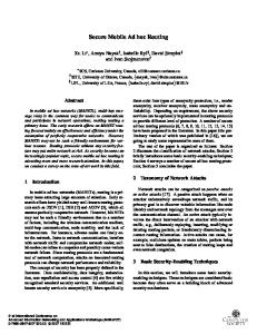
Figure 3.4: Delay of Node B and Node K CBR packets at a rate of 2 packets/sec. CBR unicast at 4 packets/sec is going from G to I, which takes path G − K − I and from F to C taking path F − B − C. DP selects node J and K to forward the broadcasts. Thus node B is forwarding only unicast traﬃc, and node K is forwarding both unicast and broadcast. As Dominant Pruning always selects node J and K to cover 2-hop neighbors {F, G, H, I}, these nodes always have a load due to the broadcast. Hence the unicast session passing via K experiences more delay than the session passing via B. This is illustrated in ﬁgure 3.4, where K has signiﬁcantly larger delay than B. Even if load aware routing protocols [24] [27] are used, unicast session from G to I could not be made better, because any path from G to I pass via at least one node from {J, A, K} and here all three of these are loaded.

There is another aspect of broadcast load balancing. Table

3.1 enlists number of packet forwards by each node. Nodes C, D, E all are relatively free while node J and K are highly loaded. This is an unfair scheduling of resources. Nodes J,K will experience faster battery depletion due to the broadcast load. So, it is expected to distribute it by

CHAPTER 3. PRELIMINARIES

34

Table 3.1: Comparison of Packet Forward by Nodes Node

Forwards

Node

Forwards

Node

Forwards

A

964

E

2

I

1

B

1993

F

1988

J

962

C

1

G

1980

K

2941

D

2

H

2

selecting the forward list between {B, K, D} and {C, J, E} to cover the 2-hop neighbors of A Thus the objective of load balanced broadcast is to distribute the broadcast load throughout the network so that the perceived load impact on other active sessions is lower and consumption of resources in various nodes are also as fair as possible. But, number of packet forwards should be kept near optimal, otherwise eﬀect of broadcast storm will dominate again.

3.5

Eﬀect of Mobility

As broadcast is unreliable, mobility doesn’t create congestion due to timeout and retransmission. But serious contention can occur due to increased node density at some regions. Neighborhood list in a node or forward list in a packet may become stale due to topology change. Result is again decreased performance.

Chapter 4 Load Aware Broadcasting 4.1

What is load aware broadcasting

To overcome the unavoidable problems of unaware broadcasting we want the broadcasting to be load aware. Here by the term ‘load aware’ we mean that a node will not transmit its broadcast packets blindly. In the previous chapter, we saw that to cover the 2-hop neighbors, a node has to select some of its neighbors as forwarding nodes for broadcasting the packets. Previous algorithms select those neighbors as forwarding nodes who are the members of minimum connected dominating sets. Here nodes are selected on the basis of neighbors. Nodes having higher number of neighbors are selected. In our approach, we also consider current network load of a node as a criteria to be selected as forwarding nodes. This is due the fact that less loaded nodes will likely transmit packets faster than heavily loaded nodes. How we integrate load and neighbor as a single selection criterion will be discussed later. Before that, we illustrate a new concept “Rank”, used later in our heuristics.

4.1.1

Rank

“Rank” is deﬁned in a bipartite graph. Consider a Bipartite graph B having partite sets1 X, Y . Without loss of generality, we can deﬁne a relation BR : X → Y from this bipartition, X being the domain, and Y 1

Refer to Appendix A : Glossary for a description of the related terms.

35

CHAPTER 4. LOAD AWARE BROADCASTING

X

36

Y

a

1/4

f

1/4

b

1/4 1/4

c

g

1/1 1/3

d

1/3

h

1/3

e

1/2

i

1/2

f

Figure 4.1: Calculation of Rank in a bipartite graph

being the range; (u, v) ∈ BR iﬀ u ∈ X, v ∈ Y and (u, v) ∈ B. For each x ∈ X, Rank of x is (x),

(x) =

1

|BR−1 (y)| y∈BR (x)

(4.1)

Here, BR (x) is the set of all y such that (x, y) ∈ BR . Similarly, BR−1 (y) is the set of all x, such that (x, y) ∈ BR . A contextual example would be, X be the set of 1-hop neighbors of a node, and Y be the set of 2-hop neighbors; the bipartite graph captures the ways a broadcast packet can reach the 2-hop neighbors from the forwarding of 1-hop neighbors. Rank of a 1-hop neighbor can be viewed as the summation of the total contributions from the 2-hop neighbors. A 2-hop neighbor u contributes

1 deg(u)

to each of the 1-hop neighbors it is

connected. Thus, the more the number of ways a 2-hop neighbor can be reached, the less it contributes to each of the 1-hop neighbor that can be used to reach it. Later we use a rank term in our heuristic “RL”, with the intuition that, the higher the rank of a 1-hop neighbor, the more “important” it is

CHAPTER 4. LOAD AWARE BROADCASTING

37

Table 4.1: Calculating contribution of each node in Y Node y ∈ Y

|BR−1 (y)| = deg(y)

f

4

g

1

h

3

i

2

Table 4.2: Calculating rank of each node in X Node x ∈ X

BR (x)

a

{f }

b

{f }

c

{f, h}

d

{f, g, h}

e

{h, i} {i}

f

(x)

1 4

1 4

1 4 1 4

+

= 0.25 = 0.25 1 3

+1+ 1 3

+ 1 2

1 2

= 0.5833 1 3

= 1.5833

= 0.8333

= 0.50

to include this neighbor in the forward list. For a supporting argument, consider node g in Figure 4.1. It can get a broadcast packet only via node d. Hence, node d must be included in the forward list. Stated another way, given that g received a broadcast packet, the probability that d was included in forward list is 1. g contributes 1 to d and makes d’s rank higher. On the other hand, consider node f . As a broadcast packet is to be delivered to all of the nodes, it must receive the packet. node f can get a broadcast packet from the broadcast of either a, b, c or d. Moreover, it is expected that f receives it only once whenever possible, i.e. including two or more elements from {a, b, c, d} in the forward list is not a desirable event in favor of f . Probability of f ’s getting it from the broadcast of either a, b, c or d is

1 4

each. Thus f contributes this amount to each of

a, b, c and d. For convenience of use with the computation of forward lists, we here-

CHAPTER 4. LOAD AWARE BROADCASTING

38

after use rank directly with bipartite graphs, with the illustrative formulation described here. Computation of rank for each of elements of X in Figure 4.1 is shown in Table 4.1 and Table 4.2.

4.2

Approaches to Load Aware Broadcasting

We propose 2 diﬀerent approaches–one is the Proactive approach and the other is the Reactive approach.

4.3

Proactive approach

In this approach, a node probabilistically distributes the forwarding responsibility of broadcasting packets among its neighbors. This selection probability is calculated on the basis of three diﬀerent heuristics. These heuristics are described below:

4.3.1

Neighbor heuristic

Let, N(x) = number of 2-hop neighbors that are neighbors of node x, N = total number of 2-hop neighbors, N(x) (4.2) N Select nodes from the set S ={x : x is a 1-hop neighbor} according P (x) =

to probability P (x). Nodes having higher probability P are likely to be selected higher number of times. So this approach can be called a probabilistic greedy neighbor approach in the sense that in greedy neighbor approach nodes with lowest neighbors are not selected at all where in probabilistic greedy neighbor approach nodes with lower neighbors rather have a lower probability to be selected. So there is a chance for every node to be selected as forwarding nodes.

CHAPTER 4. LOAD AWARE BROADCASTING

39

The procedure how the nodes are selected is similar to that of NL algorithm described in section 4.8.2, except that, rather than selecting the nodes deterministically at each iteration, a probabilistic scheme is used.

4.3.2

Rank heuristic

Let, (x) be the rank of node x,

R=

{(i) : i is a 1-hop neighbor}

(4.3)

i

P (x) =

(x) R

(4.4)

Select nodes from the set S ={x : x is a ﬁrst hop neighbor} according to probability P (x).

4.3.3

Sorted Rank heuristic

Proactive strategy could be used so that a host would try to choose neighbors in the forward list as fairly as possible. But our results show this strategy does not use queuing delay, contention and congestion at various nodes and are easily misled to wrong decisions in mobile or mixed traﬃc scenarios.

4.4

Reactive Approach

Our algorithms for load balanced broadcasting use reactive strategies to distribute the load. The reactive strategy for a node is based on creating the forward list considering the “load feedback” from neighboring nodes. Target is to select the less loaded nodes for forwarding, since it ensures balanced load distribution. The less loaded nodes do the broadcasting earlier which reduces packet transmission delay. At the same time, packets of other active sessions also experience less delay.

CHAPTER 4. LOAD AWARE BROADCASTING

4.4.1

40

Combining neighborhood information and load

While constructing the forwarding list if a node considers only load information of its neighbors, it may increase total number of packet forwarding. For example, consider the topology in ﬁgure 3.1(b). Assume node J and K have higher loads than nodes B, C, D, E and node A is broadcasting a packet. Now if it selects less loaded nodes for constructing the forwarding list, then it requires 4 nodes (i.e. B, C, D, E) to forward the packet. However, selecting {J, K} despite of their highest load requires only 2 packet forwarding. This implies that considering only load may increase packet forwarding in a large scale which may result in contention and collision in the network. Therefore, the neighborhood information of the nodes should also be considered.

4.4.2

Load incorporated Dominant Pruning - DNL and DRL

Here we describe two heuristics NL (Neighbor and Load) and RL (Rank and Load) as function of load and neighborhood information, to use with DP algorithm to ﬁnd the forward list [13]. When dominant pruning is used with NL heuristic we call it DNL (Dominant pruning with Neighbor Load) and when RL heuristic is used, we call it DRL (Dominant pruning with Rank Load. Let, the set of 1-hop neighbors of vp is N(vp ), load for vk ∈ N(vp ) is L(vk ), set of upto 2-hop neighbors of vp is N(N(vp )), set of 2-hop neighbors of vp ,

N2 (vp ) = N(N(vp )) − N(vp ) − {vp }

(4.5)

To forward a packet received from node vq , node vp builds the forward

CHAPTER 4. LOAD AWARE BROADCASTING

41

list Fp,q ⊂ X(p, q), iteratively to cover the nodes of Y (p, q) where, Xp,q = N(vp ) − {vq } − N(vq )

(4.6)

Yp,q = N2 (vp ) − N(vq ) − N(N(vq ) ∩ N(vp ))

(4.7)

At the start of iteration i, i >= 0, let the partial forward list is, Fp,q (i), (Fp,q (0) = ∅). Consider the Bipartition, Bi : Xp,q,i → Yp,q,i, where Xp,q,i = Xp,q − Fp,q (i)

(4.8)

Yp,q,i = Yp,q − N(Fp,q (i))

(4.9)

For x ∈ Xp,q,i and y ∈ Yp,q,i an edge (x, y) exists in this bipartition iﬀ y ∈ N(x). The set of nodes in Yp,q,i that are covered by x Bi (x) = {y : (x, y) ∈ E(Bi )} = N(x) ∩ Yp,q,i

(4.10)

The set of nodes in Xp,q,i that covers y B−1 i (y) = {x : (x, y) ∈ E(Bi )}

(4.11)

Among all the nodes in Xp,q,i the node vk with maximum heuristic value NL(vk , i) or RL(vk , i) (described below) is selected, and the forward list is updated as Fp,q (i + 1) = Fp,q (i) ∪ {vk }

(4.12)

NL heuristic At iteration i, NL heuristic for vk ∈ Xp,q,i is, |Bi (vk )| maxvj ∈Xp,q,i {|Bi (vj )|} maxvj ∈Xp,q,i {L(vj )} +α × L(vk )

NL(vk , i) = (1 − α) ×

(4.13)

0 <= α <= 1 is called “Load balance parameter” which determines how much emphasis is given on load balancing. If α = 0 the algorithm becomes naive greedy set cover, and if α = 1 it becomes pure load based.

CHAPTER 4. LOAD AWARE BROADCASTING

XA, J

42

YA, J

C

1/2

G

1/2

K

1/2

I

1/2

E

Figure 4.2: Calculation of Rank in the example

RL heuristic In RL heuristic, rather then taking the number of uncovered neighbors, we incorporate rank of a node in Xp,q,i. Rank for each of the node x ∈ Xp,q,i, i (x) =

1

−1 y∈Bi (x) |Bi (y)|

(4.14)

Consider in ﬁgure 3.1(b). Here N(A) = {B, C, J, K, D, E} N2 (A) = {F, H, I, G} If A is to forward a packet received from J, then vq = J, vp = A, XA,J = {C, K, E}, YA,J = {I, G}, B0 (C) = {G}, B0 (E) = {I}, B0 (K) = {I, G}. Then, (C) = 0.5, (E) = 0.5, (K) = 0.5 + 0.5 = 1. Figure 4.2 aids in this calculation. RL heuristic for vk is, i (vk ) maxvj ∈Xp,q,i {i (vj )} maxvj ∈Xp,q,i {L(vj )} +α × L(vk )

RL(vk , i) = (1 − α) ×

(4.15)

CHAPTER 4. LOAD AWARE BROADCASTING

43

SRL algorithm with RL heuristic To build the forward list, RL heuristic can be used in a diﬀerent manner resulting in a new algorithm “SRL”(Sorted Rank Load). (Algorithm 1). Instead of taking the “best” node from Xp,q,i and checking which nodes of Yp,q,i are covered, this algorithm selects node y with minimum |B−1 i (y)| −1 from Yp,q,i and covers it using nodes from B−1 i (y). If |Bi (y)| > 1, the

node with maximum RL heuristic value is selected. Algorithm 1 Procedure SRL(vp ,vq ) 1: Fp,q (0) ← ∅, Yp,q,0 ← Yp,q , 2: while Yp,q,i = ∅ do 3: Select node y ∈ Yp,q,i with minimum |B−1 i (y)| −1 4: Let S = Bi (y) 5: if |S| = 1 then 6: Select the only node vk ∈ S 7: else 8: Select vk ∈ S such that RL(vk , i) is maximum 9: end if 10: Fp,q (i + 1) ← Fp,q (i) ∪ {vk } 11: Xp,q,i+1 ← Xp,q,i − {vk } 12: Yp,q,i+1 ← Yp,q,i − N({vk }) 13: Yp,q,i+1 ← Yp,q,i − Bi (vk ) 14: i← i+1 15: end while

4.4.3

Capturing the load

To represent the load for a mobile node, utilization factor of resources like present queue length or available spaces in queue, battery power, processing capability can be used, because as an outcome of network load, resources of the hosts become loaded. Lee and Gerla [27], consider number of packets in the interface queue as a load metric. Hassanein and Zhou [25] use total number of routes passing through a node and its neighbors. On the other hand Wu and Harms [26] take summation of number of packets being queued at the

CHAPTER 4. LOAD AWARE BROADCASTING

44

mobile node and its neighboring nodes. Song et. al. [24] uses packet delay as the parameter. If the arrival and successful transmission time of the ith packet is ai and di , then they compute estimated average delay k qik = (1 − β)qi−1 + β(di − ai ) where 0 <= β <= 1, i > 1.

This delay parameter is more appropriate, since it includes both queuing delay and contention delay at the MAC layer. However, the problem with the exponential averaging equation of qik is selecting proper value of β. Delay values (di − ai ) in general contain frequent spikes. If β is large, spikes in delay value also create spikes in the average. On the other hand, small β causes delay values to be smoothed, but then the average follows any change in delay very slowly. Considering these facts, we use a moving average window W for load estimation. At time t, delay values for last Tl seconds are remembered, i.e. the averaging window is W (t) = {(di − ai ) : di >= t − Tl }

(4.16)

L(t) = Mean{W (t)}

(4.17)

Then

Experiment shows taking Tl = 5 provides excellent smoothing.

4.4.4

Exchanging load and neighborhood information

Each node piggybacks its present load information into the data packets sent or forwarded by it. This information is also piggybacked into periodic hello messages, hence an idle node also updates its load information. To pass neighborhood information, “Dynamic Hello” scheme can be used for eﬃciency. In dynamic hello scheme, instead of sending periodic hello messages, a node piggybacks neighborhood information in the data packets at ﬁxed intervals. If there is no data packet to send or forward for a predeﬁned amount of time, the node explicitly sends a hello message.

Chapter 5 Simulation Model and Evaluations 5.1

Simulation Environment

To evaluate the performance of our load balanced schemes and compare with Dominant Pruning, we have built a detailed simulation model using NS-2 [29] with wireless extensions. The physical radio characteristics are chosen to approximate Lucent WaveLAN [30] with a bit rate of 2Mbits/sec and a radio range of 250m. Propagation model used is two ray ground. For the MAC layer, IEEE 802.11 Distributed Coordination Function (DCF) [31] is used.

5.1.1

Scenario Generation

Our simulation model consists of 50 mobile hosts placed in a 1500×300m2 ﬂat area. We use random waypoint model as the mobility model. By diﬀering pause times, various degrees of mobiliy are generated. For each pause time, mean of 5 randomly generated scenario is taken. Speed of the mobile nodes are chosen to be 10ms−1 .

5.1.2

Traﬃc Generation

Our traﬃc sources are CBR. To oﬀer various degree of load in the network, 5 to 30 nodes are randomly chosen as broadcast sources, each of 45

CHAPTER 5. SIMULATION MODEL AND EVALUATIONS

46

which broadcast at a rate of 4 packets/sec. Packets are 512 bytes in size. Each simulation runs for 500 seconds of virtual time.

5.2

Performance Metrics

The performance metrics we observe are:

5.2.1

Mean Packet Forward (MPF)

MPF is average number of packet forwards by each node. Dominant pruning and other methods try to minimize number of packet forwards, while our methods try to balance the broadcast load, maintaining full reachability (covering all required 2-hop neighbors). We observe MPF to check how much extra packet forward is incurred on average due to load balancing. MP F =

5.2.2

Total number of packet forwards Total nodes

(5.1)

Standard deviation of Packet Forward (SPF)

SPF is the standard deviation (STD) of number of packets forwarded by each node. This is the main metric we observe as the “quality” of load balancing. Better load balancing implies less value of SPF. However, to ensure 100% reachability and due to dynamic condition of the network, SPF value may show large deviation, even if load balance is used. If n is the number of total nodes and P Fi is total number of packets forwarded by node i then,

(P Fi − MP F )2 (5.2) n−1 We include this metric to test the fairness of distribution of load among SP F =

n i=1

several nodes.

5.2.3

Average Broadcast Latency (ABL)

It is the mean interval from the time a broadcast packet is initiated to the time the last host receiving it. We observe this metric, as it speciﬁes

CHAPTER 5. SIMULATION MODEL AND EVALUATIONS

47

an important performance issue of a broadcast protocol, the maximum delay between send and receive that can occur on average.

ABL =

5.3

i (Time

the last host received pkti - Time pkti was sent) Total number of broadcast packets (5.3)

Simulation Results

We compare the performance of DNL, DRL and SRL with DP algorithm. Value of α is taken 0.15. By experiments, we ﬁnd that choosing alpha between 0.1 to 0.3 does excellent load balancing without costing too many extra packet forwards.

5.3.1

Performance vs. Mobility

Here we evaluate the outcome of load balancing as a function of varying mobility. We simulated the models with pause times from 0 to 500 seconds with an interval of 50 seconds. We show and explain each of the performance metric for six diﬀerent load conditions. Our experiment consisted of using 5, 10, 15, 20, 25 and 30 sources. As each node generates broadcast packets at a rate of 4 packets/sec, having 5 broadcast source means an aggregate of 5 × 4 = 20 packets/sec in the network, 15 broadcast source means 60 packets/sec, and so on. When load in the network is 20-40 packets/sec we call denote it as “low load” condition. Similarly 60-80 packets/sec is termed as “Medium load” and 100-120 packets/sec as “High Load”. MPF Figure 5.1, 5.2 and 5.3 show MPF for varying mobility. For low load conditions, each of the algorithms perform similar for all degree of mobility. The general trend of all of the algorithms with respect to mobility is that, number of packet forwards increase as mobility decreases when load is low. As we can see from Figure 5.2(b) and Figure

CHAPTER 5. SIMULATION MODEL AND EVALUATIONS

48

5.3(b), when mobility is high (pause time low), the performance is somehow unpredictable. This is intuitive because due to random change in topology, random behavior among the algorithms are expected. However DNL is inferior to the other three in case of number of packet forwards, which is clearly visible in Figure 5.2 and 5.3. Figure 5.3(b) shows that Dominant pruning dominates the other three in reducing the number of packet forwards in highly mobile environments. As mobility decreases, diﬀerence in number of packet forward decreases also. SRL seems to outperform DRL, in almost all degrees of mobility and again, this diﬀerence decreases with decreasing mobility. One subtle point is also clear from Figure 5.3. While the low and medium load graphs of Figure 5.1 and Figure 5.2 showed increase in number of packet forwards as pause time increased, the high load condition of Figure 5.3 shows decrease in this number as pause time is increased. We can call it a “Behavior-inversion” phenomena. In fact Figure 5.2(b) can be observed as the transition between two trends. The reason we think is that–When load is high, there are too many packet forwarding attempts in small amount of time which results in medium contention and corrupted packets due to collision. This increases in number of packet forwards. On the other hand, when load is low, medium contention and collision is also low. In both cases, when mobility is high, wrong decisions are taken (a 1-hop neighbor forwards a packet in the hope to reach a 2-hop neighbor, but if the 2-hop neighbor goes out of range in the meantime the forwarding may be unnecessary). But for the high load case, wrong decisions lead to more collisions and corrupted packets. SPF Figure 5.4, 5.5 and 5.6 show SPF for varying mobility. DNL algorithm, which is the outcome of incorporating NL heuristic in Dominant pruning algorithm, clearly showed worst performance in case of MPF. However, its high packet forward is justiﬁed in 5.6(a) and Figure 5.6(b), where DNL clearly outperforms the rest two in SPF. DRL and SRL perform

CHAPTER 5. SIMULATION MODEL AND EVALUATIONS

49

almost similar in balancing the load. As one can imagine, DP performs worst here, as there is no load balancing scheme incorporated. Diﬀerence of SPF between load balanced schemes and DP is low in highly mobile environments. This is because, dynamically changing neighborhood list due to mobility, unconsciously does some load balancing here. In fact, for all of the algorithms, mobility related “unconscious” load balancing helps decreasing SPF. Thus the trend of SPF with varying mobility is same for all load conditions. As mobility increases, SPF decreases, and as mobility decreases SPF increases. ABL Figure 5.7, 5.8 and 5.9 show ABL for varying mobility. Latency shows similar trend to MPF with varying mobility, when load is low in Figure 5.7. As load increases in Figure 5.8 and 5.9, DRL and SRL seem to outperform DP and DNL and reduce latency as mobility decreases. Latency decreases with decreasing mobility for all schemes, when load is high. However “Behavior-inversion” phenomena like MPF is observed here also. Considering latency, performance of DNL is worst here. Trend of the metrics with respect to mobility is almost same for all schemes. This behavior is also expected, as each of the proposed schemes are based on the fundamental set cover idea of DP.

5.3.2

Varying number of sources

Here we evaluate the performance, as a function of network load. We vary the load by varying number of broadcast sources. We show and explain the performance for nine diﬀerent pause times. These pause times are taken as 0, 50, 100, 200, 250, 300, 400, 450, 500 seconds. Graphs of each performance metric are shown for three diﬀerent mobility scenarios high, medium and low. Pause times 0, 50 and 100 seconds are considered as high mobility scenarios. Pause times 200, 250 and 300 seconds are considered as medium mobility scenarios and pauses times

CHAPTER 5. SIMULATION MODEL AND EVALUATIONS

50

400, 450 and 500 seconds are taken as low mobility scenarios. Each performance parameter is analyzed below: MPF Figure 5.10, 5.11 and 5.12 show MPF for varying number of sources. From these ﬁgures, we see that MPF of all algorithms are approximately equal for less than 15 sources when mobility is high, for less then 20 sources when mobility is medium and for less than 25 sources when mobility is very low (pause time=500 seconds). That is there is no signiﬁcant diﬀerence in MPF when number of sources is less then a particular value which is 15 for high mobile, 20 for medium mobile and 25 for low mobile scenario. Moreover, this particular value increases with decrease in mobility (increase in pause time). This also implies that when network load (which is the combination of source and mobility) is less than a particular threshold, all algorithms give similar performance. However, when load in the network crosses this threshold, the behavior starts to change. For number of sources greater than the particular value when load in the network increases, DNL algorithm produces larger packet forwards then the other three algorithms. However, DP, DRL and SRL produce approximately equal number of packet forwards showing no signiﬁcant diﬀerence in behavior. Moreover, we see that these behaviors also do not change much with changes in mobility. The same shape of the graphs for high, medium and low mobility justiﬁes this. SPF Figure 5.13, 5.14 and 5.15 show SPF for various load conditions. Here DP algorithm performs worse load balancing producing larger SPF in all mobility and load conditions. DNL algorithm outperforms other three considering SPF. It is expected since it distributes load in a more balanced way than the other three algorithms in the network. However, DRL and SRL algorithms perform approximately similar. Since DP performs no load balancing in the network it produces worse SPF in all

CHAPTER 5. SIMULATION MODEL AND EVALUATIONS

51

conditions. However, comparing Figure 5.13, 5.14 and 5.15, we observe that the diﬀerence of SPF between DP and other three algorithms increases as mobility decreases. This diﬀerence is lowest when mobility is high as seen in Figure 5.13 and largest when mobility is low as seen in Figure 5.15. This is due to the reason that increased mobility results in dynamically changing neighbor list which unconsciously does some load balancing. ABL Figure 5.16, 5.17 and 5.18 show ABL for varying number of sources. From these ﬁgures we see that, all four algorithms perform similar considering ABL for less than 15 sources when mobility is high, for less then 20 sources when mobility is medium and for less than 25 sources when mobility is very low(pause time=500 seconds) . That is there is no signiﬁcant diﬀerence in ABL when number of sources is less then a particular value which is 15 for high mobile, 20 for medium mobile and 25 for low mobile scenario. Moreover, this particular value increases with decrease in mobility (increase in pause time). This also implies that when network load (which is the combination of source and mobility) is less than a particular threshold, all algorithms gives similar performance. However, when load in the network crosses this threshold, the behavior starts to change. For number of sources greater than this when load in the network increases, DNL algorithm produces larger delays than other three algorithms as seen from those ﬁgures. However, DP, DRL and SRL produce approximately similar delays showing no signiﬁcant diﬀerence in behavior. From these ﬁgures we see however that, SRL and DP are both competitive in their behavior, but SRL produces lesser values than DP and shows the best performance in minimizing the latency. In all simulations, DNL shows decreased performance considering Number of packet forwards and Average broadcast latency. However, it tends to distribute the load more and decrease SPF, but to that extent, that it hurts other performance parameters. In fact, RL heuristic

CHAPTER 5. SIMULATION MODEL AND EVALUATIONS

52

performs far better than NL, and SRL gives nearly optimal packet forwards, better load balancing and decreased latency with respect to DP over various load conditions.

CHAPTER 5. SIMULATION MODEL AND EVALUATIONS

1300

Mean packet forward

1200

53

DP DNL DRL SRL

1100

1000

900

800

700 0

100

200 300 Pause time

400

500

400

500

(a) MPF, 5 sources

2000 1900

DP DNL DRL SRL

Mean packet forward

1800 1700 1600 1500 1400 1300 1200 0

100

200 300 Pause time (b) MPF, 10 sources

Figure 5.1: MPF vs. Pause time for low load (20-40 packets/sec)

CHAPTER 5. SIMULATION MODEL AND EVALUATIONS

2400

Mean packet forward

2300

54

DP DNL DRL SRL

2200 2100 2000 1900 1800 1700 0

100

200 300 Pause time

400

500

400

500

(a) MPF, 15 sources

3400

Mean packet forward

3200

DP DNL DRL SRL

3000

2800

2600

2400

2200 0

100

200 300 Pause time (b) MPF, 20 sources

Figure 5.2: MPF vs. Pause time for medium load (60-80 packets/sec)

CHAPTER 5. SIMULATION MODEL AND EVALUATIONS

55

4600 DP DNL DRL SRL

4400

Mean packet forward

4200 4000 3800 3600 3400 3200 3000 2800 2600 0

100

200 300 Pause time

400

500

(a) MPF, 25 sources

5500

DP DNL DRL SRL

Mean packet forward

5000

4500

4000

3500

3000

2500 0

100

200 300 Pause time

400

500

(b) MPF, 30 sources

Figure 5.3: MPF vs. Pause time for high load (100-120 packets/sec)

CHAPTER 5. SIMULATION MODEL AND EVALUATIONS

2000 1800

STD of packet forward

1600

56

DP DNL DRL SRL

1400 1200 1000 800 600 400 200 0

100

200 300 Pause time

400

500

400

500

(a) SPF, low load (5 sources)

3000

STD of packet forward

2500

DP DNL DRL SRL

2000

1500

1000

500

0 0

100

200 300 Pause time

(b) SPF, low load (10 sources)

Figure 5.4: SPF vs. Pause time for low load (20-40 packets/sec)

CHAPTER 5. SIMULATION MODEL AND EVALUATIONS

4000

STD of packet forward

3500

57

DP DNL DRL SRL

3000 2500 2000 1500 1000 500 0

100

200 300 Pause time

400

500

400

500

(a) SPF, medium load (15 sources)

4500

STD of packet forward

4000

DP DNL DRL SRL

3500 3000 2500 2000 1500 1000 0

100

200 300 Pause time

(b) SPF, medium load (20 sources)

Figure 5.5: SPF vs. Pause time for medium load (60-80 packets/sec)

CHAPTER 5. SIMULATION MODEL AND EVALUATIONS

5000

STD of packet forward

4500

58

DP DNL DRL SRL

4000 3500 3000 2500 2000 1500 1000 0

100

200 300 Pause time

400

500

400

500

(a) SPF, high load (25 sources)

5000

STD of packet forward

4500

DP DNL DRL SRL

4000 3500 3000 2500 2000 1500 0

100

200 300 Pause time

(b) SPF, high load (30 sources)

Figure 5.6: SPF vs. Pause time for high load (100-120 packets/sec)

CHAPTER 5. SIMULATION MODEL AND EVALUATIONS

0.062 0.06 Average Broadcast Latency

0.058

59

DP DNL DRL SRL

0.056 0.054 0.052 0.05 0.048 0.046 0.044 0.042 0.04 0

100

200 300 Pause time

400

500

400

500

(a) ABL, low load (5 sources)

Average Broadcast Latency

0.07

0.065

DP DNL DRL SRL

0.06

0.055

0.05

0.045 0

100

200 300 Pause time

(b) ABL, low load (10 sources)

Figure 5.7: ABL vs. Pause time for low load (20-40 packets/sec)

CHAPTER 5. SIMULATION MODEL AND EVALUATIONS

Average Broadcast Latency

0.08

0.075

60

DP DNL DRL SRL

0.07

0.065

0.06

0.055 0

100

200 300 Pause time

400

500

(a) ABL, medium load (15 sources)

1.8 DP DNL DRL SRL

Average Broadcast Latency

1.6 1.4 1.2 1 0.8 0.6 0.4 0.2 0 0

100

200 300 Pause time

400

500

(b) ABL, medium load (20 sources)

Figure 5.8: ABL vs. Pause time for medium load (60-80 packets/sec)

CHAPTER 5. SIMULATION MODEL AND EVALUATIONS

61

4.5 DP DNL DRL SRL

Average Broadcast Latency

4 3.5 3 2.5 2 1.5 1 0.5 0 0

100

200

300

400

500

Pause time (a) ABL, high load (25 sources)

6

DP DNL DRL SRL

Average Broadcast Latency

5

4

3

2

1

0 0

100

200

300

400

500

Pause time (b) ABL, high load (30 sources)

Figure 5.9: ABL vs. Pause time for high load (100-120 packets/sec)

CHAPTER 5. SIMULATION MODEL AND EVALUATIONS 5500

Mean packet forward

DP 5000 DNL DRL 4500 SRL 4000 3500 3000 2500 2000 1500 1000 500 5

10

15 20 Number of sources

25

30

25

30

25

30

(a) MPF, (Pause time = 0 sec) 5000

Mean packet forward

DP DNL 4500 DRL SRL 4000 3500 3000 2500 2000 1500 1000 500 5

10

15 20 Number of sources

(b) MPF, (Pause time = 50 sec) 5000

Mean packet forward

DP DNL 4500 DRL SRL 4000 3500 3000 2500 2000 1500 1000 500 5

10

15 20 Number of sources

(c) MPF, (Pause time = 100 sec)

Figure 5.10: MPF vs. number of sources for high mobility

62

CHAPTER 5. SIMULATION MODEL AND EVALUATIONS 4500

Mean packet forward

DP DNL 4000 DRL SRL 3500 3000 2500 2000 1500 1000 5

10

15 20 Number of sources

25

30

25

30

25

30

(a) MPF, (Pause time = 200 sec) 4500

Mean packet forward

DP DNL 4000 DRL SRL 3500 3000 2500 2000 1500 1000 5

10

15 20 Number of sources

(b) MPF, (Pause time = 250 sec) 4500

Mean packet forward

DP DNL 4000 DRL SRL 3500 3000 2500 2000 1500 1000 5

10

15 20 Number of sources

(c) MPF, (Pause time = 300 sec)

Figure 5.11: MPF vs. number of sources for medium mobility

63

CHAPTER 5. SIMULATION MODEL AND EVALUATIONS 4000

Mean packet forward

DP DNL DRL 3500 SRL 3000

2500

2000

1500

1000 5

10

15 20 Number of sources

25

30

25

30

25

30

(a) MPF, (Pause time = 400 sec) 4000

Mean packet forward

DP DNL DRL 3500 SRL 3000

2500

2000

1500

1000 5

10

15 20 Number of sources

(b) MPF, (Pause time = 450 sec) 4000

Mean packet forward

DP DNL DRL 3500 SRL 3000

2500

2000

1500

1000 5

10

15 20 Number of sources

(c) MPF, (Pause time = 500 sec)

Figure 5.12: MPF vs. number of sources for low mobility

64

CHAPTER 5. SIMULATION MODEL AND EVALUATIONS 3000

STD of packet forward

DP DNL DRL 2500 SRL 2000

1500

1000

500

0 5

10

15 20 Number of sources

25

30

25

30

25

30

(a) SPF, (Pause time = 0 sec) 3000

STD of packet forward

DP DNL DRL 2500 SRL 2000

1500

1000

500

0 5

10

15 20 Number of sources

(b) SPF, (Pause time = 50 sec) 3000

STD of packet forward

DP DNL DRL 2500 SRL 2000

1500

1000

500

0 5

10

15 20 Number of sources

(c) SPF, (Pause time = 100 sec)

Figure 5.13: SPF vs. number of sources for high mobility

65

CHAPTER 5. SIMULATION MODEL AND EVALUATIONS 2800

STD of packet forward

DP 2600 DNL DRL 2400 SRL 2200 2000 1800 1600 1400 1200 1000 800 600 5

10

15 20 Number of sources

25

30

25

30

25

30

(a) SPF, (Pause time = 200 sec) 3500

STD of packet forward

DP DNL DRL 3000 SRL 2500

2000

1500

1000

500 5

10

15 20 Number of sources

(b) SPF, (Pause time = 250 sec) 3500

STD of packet forward

DP DNL DRL 3000 SRL 2500

2000

1500

1000

500 5

10

15 20 Number of sources

(c) SPF, (Pause time = 300 sec)

Figure 5.14: SPF vs. number of sources for medium mobility

66

CHAPTER 5. SIMULATION MODEL AND EVALUATIONS 3500

STD of packet forward

DP DNL DRL 3000 SRL

2500

2000

1500

1000 5

10

15 20 Number of sources

25

30

25

30

25

30

(a) SPF, (Pause time = 400 sec) 4000

STD of packet forward

DP DNL DRL 3500 SRL 3000

2500

2000

1500

1000 5

10

15 20 Number of sources

(b) SPF, (Pause time = 450 sec)

STD of packet forward

5000

DP DNL 4500 DRL SRL 4000 3500 3000 2500 2000 1500 1000 5

10

15 20 Number of sources

(c) SPF, (Pause time = 500 sec)

Figure 5.15: SPF vs. number of sources for low mobility

67

CHAPTER 5. SIMULATION MODEL AND EVALUATIONS 6

Average Broadcast Latency

DP DNL DRL 5 SRL 4

3

2

1

0 5

10

15 20 Number of sources

25

30

25

30

25

30

(a) ABL, (Pause time = 0 sec)

Average Broadcast Latency

5

DP 4.5 DNL DRL 4 SRL 3.5 3 2.5 2 1.5 1 0.5 0 5

10

15 20 Number of sources

(b) ABL, (Pause time = 50 sec)

Average Broadcast Latency

4.5

DP DNL 4 DRL SRL 3.5 3 2.5 2 1.5 1 0.5 0 5

10

15 20 Number of sources

(c) ABL, (Pause time = 100 sec)

Figure 5.16: ABL vs. number of sources for high mobility

68

CHAPTER 5. SIMULATION MODEL AND EVALUATIONS

Average Broadcast Latency

4

DP DNL 3.5 DRL SRL 3 2.5 2 1.5 1 0.5 0 5

10

15 20 Number of sources

25

30

25

30

25

30

(a) ABL, (Pause time = 200 sec) 3

Average Broadcast Latency

DP DNL DRL 2.5 SRL 2

1.5

1

0.5

0 5

10

15 20 Number of sources

(b) ABL, (Pause time = 250 sec) 3.5

Average Broadcast Latency

DP DNL 3 DRL SRL

2.5 2 1.5 1 0.5 0 5

10

15 20 Number of sources

(c) ABL, (Pause time = 300 sec)

Figure 5.17: ABL vs. number of sources for medium mobility

69

CHAPTER 5. SIMULATION MODEL AND EVALUATIONS

Average Broadcast Latency

2

DP 1.8 DNL DRL 1.6 SRL 1.4 1.2 1 0.8 0.6 0.4 0.2 0 5

10

15 20 Number of sources

25

30

25

30

25

30

(a) ABL, (Pause time = 400 sec)

Average Broadcast Latency

2

DP 1.8 DNL DRL 1.6 SRL 1.4 1.2 1 0.8 0.6 0.4 0.2 0 5

10

15 20 Number of sources

(b) ABL, (Pause time = 450 sec)

Average Broadcast Latency

2

DP 1.8 DNL DRL 1.6 SRL 1.4 1.2 1 0.8 0.6 0.4 0.2 0 5

10

15 20 Number of sources

(c) ABL, (Pause time = 500 sec)

Figure 5.18: ABL vs. number of sources for low mobility

70

Chapter 6 Conclusions We have discussed a new problem–load aware broadcasting. We have shown why it is necessary to balance the broadcast load and proposed two new heuristics–NL and RL, to calculate the forward list in DP algorithm. A new algorithm SRL employing heuristic RL is proposed also, which calculates the forward list in a diﬀerent manner than DP. Simulation results show that, our methods decrease SPF by more than 30% in a medium loaded environment while keeping MPF near optimal, and this performance is even better with increased load. Moreover, end to end delay, jitter, latency and other performance parameters improve also. Hence our method is perfectly applicable to a wide spectrum starting from low load conditions to high load broadcasting needs. There are scopes for further extensions of our work. Here we simulated our schemes for CBR traﬃc models only. But there can be performance variations in biased traﬃc or topology conditions. For example, web traﬃc is observed to follow zipf law [32]. Client/Server model can be considered to have exponentially distributed traﬃc. So, more realistic traﬃc models can be used in special scenarios. We considered only broadcast sessions. But performance of mixed unicast and broadcast sessions, and eﬀect of unicast on broadcast and vice versa can be experimented also. Moreover, as our load aware broadcast tries to distribute the broadcast load, broadcast intensive applications can be simulated also. There can be much variations in these 71

CHAPTER 6. CONCLUSIONS

72

schemes. For example, experimental data can be collected from applications like real time audio-video conferencing, collaborative computing, video streaming over ad hoc networks and appropriate models can be ﬁtted to predict a probability distribution of those traﬃc. Using these distributions, performance of our load aware broadcasting can be examined. Not only various traﬃc models, but eﬀect of topology can be examined also. We assumed uniform distribution of mobile nodes in a rectangular region. But C-shaped, H-shaped, L-shaped or zipf distributed topology also arises in practical situations. Hence we can test the performance in these specialized topology models also.

Appendix A Glossary A.1

Graph

A graph G is a triple consisting of a vertex set V (G), an edge set E(G), and a relation that associates with each edge two vertices (not necessarily distinct) called its endpoints. Figure 3.1(b) is an example of a graph with the vertex set, V ={A, B, C, D, E, F, G, H, I, J, K}.

A.2

Graph model of a network

By the term “node”, in this paper we mean the network stations (example can be a personal computer, laptop computer, cell phone i.e. a device with computational and networking capability), which can perform some network activity. A network topology can mathematically be modeled as a graph. The set of all the “networking capable devices” or the “stations” be the vertice set, and the set of all the interconnections between the stations be the edge set. In an ad hoc wireless network, all the network stations x physically in the radio range of a network station a will cause the corresponding topology graph to have undirected edge (a, x). Figure 3.1(a) shows physical position of mobile nodes, their radio range as gray circular regions around each node, and corresponding topology graph is shown in Figure 3.1(b).

73

APPENDIX A. GLOSSARY

74

In Figure 3.1(b) the edge (A, B) means network node A and network node B are in the radio range of each other; A can receive B’s transmissions and vice versa (assume without loss of generality, both of them has same radio range). If the radio range is not same for A and B, then the underlying topology graph will have directed edges, where (u, v) means node v can hear the transmissions from node u but not necessarily vice versa.

A.3

MAC sublayer for MANET

Nodes in an ad hoc wireless network use a shared broadcast radio channel. To transmit a frame, the sender must broadcast it on the air. All the nodes in the radio range of the sender can listen to that transmission if an omnidirectional antenna is used. The wireless medium can be considered as a shared ‘resource’ with ‘read’ and ‘write’ operations. Like shared ethernet, transmissions (the write operation) should be mutually exclusive to prevent a node from corrupting another node’s ongoing transmission, while reception (the read operation) do not need such restrictions. However, due to several issues associated with wireless media, a specialized Medium Access Control (MAC) is needed. IEEE 802.11 DCF IEEE 802.11 MAC uses a Carrier Sense Multiple Access / Collision Avoidance (CSMA/CA) scheme. Collision avoidance is actually diﬃcult in MANET due to hidden station and exposed station problems. To account for hidden station and exposed station problems, RTS (Request To Send), CTS (Clear To Send), Data and ACK frames are used for unicast packets. But they are both complex and expensive to implement for broadcasting. The condition a broadcasting node need to meet is that they assess a clear channel before broadcasting. This scheme does not prevent collision. Unless speciﬁc means are implemented at the upper layer, a node can not determine whether a packet was successfully reached by its neighbors.

APPENDIX A. GLOSSARY

75

In congested networks, signiﬁcant amount of collisions occur leading to higher packet dropping rate. Broadcasting protocols try to limit the probability of collisions by limiting the number of rebroadcasts in the network [15].

A.4

Delay Jitter

In networking terms, “Delay Jitter” or “Packet Delay Variation” (PDV) is deﬁned in RFC 3393. It is the end to end delay between selected packets in a ﬂow with any lost packets being ignored [33]. The delay is speciﬁed from the start of the packet being transmitted at the source to the end of the packet being received at the destination. But broadcast protocols add a random jitter to the scheduled time of the retransmission of a broadcast packet. If the artiﬁcial delay is not added, MAC performance degrade. After receiving a broadcast packet at almost same time, several nodes examine the medium at the same time to ﬁnd it free and start retransmission at the same time resulting in collision. The added delay decreases the probability of this event.

A.5

RAD

Many broadcasting protocols require a node to keep track of redundant packets received over a short time interval in order to determine whether to rebroadcast. That time interval is termed Random Assessment Delay (RAD). RAD is an uniform random number U (0, Tm ax) seconds.

A.6

Subgraph

A subgraph of a graph G is a graph H such that V (H) ⊆ V (G) and E(H) ⊆ E(G) and the assignment of endpoints to edges in H is the same as in G. We then write H ⊆ G and say that “G contains H”. A graph is connected if each pair of vertices in G belongs to a path; otherwise, G is disconnected.

APPENDIX A. GLOSSARY

76

Figure A.1: Minimum Dominating Set in a Graph

A.7

Independent Set

An independent set or stable set in a graph is a set of pairwise nonadjacent vertices. In Figure reftopology {F, G, H, I} is an independent set.

A.8

Bipartite Graph

A graph G is bipartite [34] if V (G) is the union of two disjoint (possibly empty) independent sets called partite sets of G. Figure 4.1 shows a bipartite graph with partite sets X and Y .

A.9

Bipartition

A bipartition [34] of G is a speciﬁcation of two disjoint independent sets in G whose union is V (G). The statement “Let G be a bipartite graph with bipartition X,Y ” speciﬁes one such partition. An X,Y -bigraph is a bipartite graph with bipartition X,Y . The sets of a bipartition are partite sets. A disconnected bipartite graph has more than one bipartition. A connected bipartite graph has only one bipartition, except for interchanging the two sets.

A.10

Dominating Set

In a graph G, a set S ⊆ V (G) is a dominating set if every vertex not in S has a neighbor in S. The domination number γ(G) [34] is the minimum size of a dominating set in G.

APPENDIX A. GLOSSARY

77

In the graph of Figure A.1 the squared vertices constitute a minimum dominating set. Hence γ(G) = 3 for this graph. However, the set of the squared vertices is not a MCDS or Minimum Connected Dominating Set as G[S] is not connected. The closed neighborhood N[v] of a vertex v in a graph is N(v) ∪ {v}; it is the set of vertices dominated by v. A dominating set S in G is 1. A connected dominating set if G[S] is connected, 2. an independent dominating set if G[S] is independent, and 3. a total dominating set if G[S] has no isolated vertex.

A.11

Set Cover

A Set cover is set of sets whose union has all members of the union of all sets [35]. Formally, given a universe U and a family S of subsets of U, a set cover is a subfamily C ⊆ U of sets, whose union is U. The set cover problem is to ﬁnd a minimum size set. The greedy algorithm for set covering chooses sets according to one rule: at each stage, choose the set which contains the largest number of uncovered elements. It can be shown that this algorithm achieves an approximation ratio of H(s), where s is the size of the largest set and H(n) is the n-th harmonic number: H(n) =

n

1 ≤ ln n + 1 k=1 k

APPENDIX A. GLOSSARY Table A.1: Meaning of the abbreviations used in this text Term

Meaning

ABL

Average Broadcast Latency

ACK

Acknowledgment

AHBP

Ad Hoc Broadcast Algorithm

AODV

Ad hoc On-demand Distance Vector

CBRP

Cluster Based Routing Protocol

CDS

Connected Dominating Set

CSMA

Carrier Sense Multiple Access

CTS

Clear To Send

DCF

Distributed Coordinate Function

DNL

Dominant Pruning with Neighbor Load

DP

Dominant Pruning

DRL

Dominant Pruning with Rank Load

DSDV

Destination-Sequenced Distance Vector

DSR

Dynamic Source Routing

DVMRP

Distance Vector Multicast Routing Protocol

LAR

Location Aided Routing

MAC

Medium Access Control

MANET

Mobile Ad hoc Network

MCDS

Minimum Connected Dominating Set

MPF

Mean Packet Forward

MR

Multipoint Relaying

NL

Neighbor and Load

PDV

Packet Delay Variation

RAD

Random Assessment Delay

RL

Rank and Load

RTS

Request To Send

SBA

Scalable Broadcast Algorithm

SP

Self Pruning

SPF

Standard deviation of number of Packet Forward

SRL

Sorted Rank Load

ZRP

Zone Routing Protocol

78

Bibliography [1] C. S. R. Murthy and B. S. Manoj, Ad Hoc Wireless Networks Architectures and Protocols, 1st ed. Delhi, India: Pearson Education Inc. and Dorling Kindersley Publishing Inc., 2004, pp. 213–248. [2] A. S. Tanenbaum, Computer Networks, 4th ed. Upper Saddle River, New Jersey 07458, U.S.A: Pearson Education Inc., 2003, pp. 372– 380. [3] Wikipedia, “Suran — wikipedia, the free encyclopedia,” 2008, [Online;

accessed 1-March-2009]. [Online]. Available:

http:

//en.wikipedia.org/w/index.php?title=SURAN&oldid=248320105 [4] C. Toh, Ad Hoc Mobile Wireless Networks.

Upper Saddle River,

New Jersey 07458, U.S.A: Prentice-Hall, Inc., 2001. [5] “Mobile ad-hoc networks (manet),” IETF MANET working group charter. [Online]. Available:

http://www.ietf.org/html.charters/

manet-charter.html [6] E. Royer and C.-K. Toh, “A review of current routing protocols for ad-hoc mobile wireless networks,” IEEE Person. Commun., vol. 6, no. 2, Apr 1999. [7] C. Perkins and P. Bhagwat, “Routing over multihop wireless network of mobile computers,” in SIGCOMM ’94: Computer Communications Review, vol. 24, no. 4, Oct 1994, pp. 234–244. [8] M. Jiang, J. Li, and Y. Tay, “Cluster based routing protocol (CBRP) functional speciﬁcation,” 1998, internet Draft. 79

BIBLIOGRAPHY

80

[9] C. Perkins, E. Royers, and S. Das, “Ad-hoc On-demand Distance Vector Routing (AODV),” February 2003, internet Draft: draft-ietfmanet-aodv-13.txt. [10] D. Johnson and D. Maltz, “Dynamic source routing in ad-hoc wireless networks,” in Computer Communications Review- Proceedings of SIGCOMM ’96, August 1996. [11] Z. Haas and M. Pearlman, “The zone routing protocol (ZRP) for ad hoc networks,” 1998, internet Draft. [12] E. Royer and C. E. Perkins, “Multicast operation of the ad-hoc on-demand distance vector routing protocol,” in Proceedings of MobiCom ’99, Seattle, WA, USA, Aug 1999, pp. 207–218. [13] H. Lim and C. Kim, “Multicast tree construction and ﬂooding in wireless ad hoc networks,” in Proc. ACM MSWiM, USA, 2000, pp. 61–68. [14] M. D. Colagrosso, “Intelligent broadcasting in mobile ad hoc networks: Three classes of adaptive protocols,” EURASIP Journal on Wireless Communications and Networking, vol. 2007, no. 10216, 2007. [15] B. Williams and T. Camp, “Comparison of broadcasting techniques for mobile ad hoc networks,” in Proc. 3rd ACM Int. Symposium on Mobile ad hoc networking & computing, Switzerland, 2002. [16] S. Das, C. Perkins, and E. Royer, “Performance comparison of two on-demand routing protocols for ad hoc networks,” in Proc. IEEE INFOCOM, March 2000, pp. 3–12. [17] Y. Ko and N. Vaidya, “Location-aided routing (LAR) in mobile ad hoc networks,” in Proc. IEEE/ACM International Conference on Mobile Computing and Networking MobiCom, 1998, pp. 66–75.

BIBLIOGRAPHY

81

[18] S. Ni, Y. Tseng, Y. Chen, and J. Sheu, “The broadcast storm problem in a mobile ad hoc network,” in Proc. MobiCom, USA, 1999, pp. 151–162. [19] W. Peng and X. Lu, “On the reduction of broadcast redundancy in mobile ad hoc networks,” in Proceedings of MobiHoc 2000, MA, USA, 2000. [20] A. Qayyum, L. Viennot, and A. Laouiti, “Multipoint relaying: An eﬃcient technique for ﬂooding in mobile wireless networks,” INRIA, France, Technical Report 3898 - Rapport de recherche, 2000. [21] W. Peng and X. Lu, “AHBP: An eﬃcient broadcast protocol for mobile Ad hoc networks,” Journal of Computer Science and Technology, vol. 16, no. 2, pp. 114–125, March 2001. [22] J. Sucec and I. Marsic, “An eﬃcient distributed network-wide broadcast algorithm for mobile ad hoc networks,” CAIP Center, Rutgers University, Piscataway, NJ, USA, CAIP Technical Report 248, 2000. [23] W. Peng and X. Lu, “Eﬃcient broadcast in mobile ad hoc networks using connected dominating sets,” Journal of Software, 1999. [24] J. Song, V. Wong, and V. Leung, “Load-aware on-demand routing (LAOR) protocol for mobile ad hoc networks,” in Proc. The 57th IEEE Semiannual VTC, Jeju, Korea, April 2003. [25] H. Hassanein and A. Zhou, “Routing with load balancing in wireless ad hoc networks,” in Proc. ACM MSWiM, Italy, June 2001. [26] K. Wu and J. Harms, “Load-sensitive routing for mobile ad hoc networks,” in Proc. IEEE ICCCN, Scottsdale, AZ, October 2001. [27] S. Lee and M. Gerla, “Dynamic load-aware routing in ad hoc networks,” in Proc. IEEE ICC’01, Finland, June 2001.

BIBLIOGRAPHY

82

[28] C. Ho, K. Obraczka, G. Tsudik, and K. Viswanath, “Flooding for reliable multicast in multi-hop ad hoc networks,” in Proceedings of the International workshop on Discrete algorithms and methods for mobile computing and communication (DIALM), 1999, pp. 64–71. [29] “The Network Simulator:

NS-2:

notes and documentation.”

[Online]. Available: http://www.isi.edu/nsnam/ns/ [30] “Development of WaveLAN, an ISM band Wireless LAN,” July/Aug 1993, AT&T Technical Journal. [31] IEEE Standards Department, “Wireless LAN medium access control (MAC) and physical layer (PHY) speciﬁcations,” 1997, IEEE standard 802.11-1997. [32] L. A. Adamic and B. A. Huberman, “Zipfs law and the internet,” Glottometrics 3, pp. 143–150, 2002. [33] C. Demichelis and P. Chimento, “IP Packet Delay Variation metric for IP performance metrics (IPPM),” Nov 2002, network Working Group draft-ietf-ippm-ipdv. [Online]. Available:

http:

//tools.ietf.org/html/rfc3393 [34] D. B. West, Introduction to Graph Theory, 2nd ed.

Upper Saddle

River, New Jersey 07458, U.S.A: Prentice-Hall, Inc., 2001, pp. 1–30. [35] Wikipedia, “Set cover problem — wikipedia, the free encyclopedia,” line].

2009,

Available:

[Online;

accessed

1-March-2009].

[On-

http://en.wikipedia.org/w/index.php?title=

Set cover problem&oldid=274428703