©2009 The Visualization Society of Japan Journal of Visualization, Vol. 12, No. 1 (2009) 27-35
Measurement of Pressure Distribution from PIV Experiments
Jaw, S.Y. *1, Chen, J.H. *1, and Wu, P.C. *1 *1 Department of Systems Engineering and Naval Architecture, National Taiwan Ocean University, Keelung, Taiwan. E-mail:
[email protected] Received 22 November 2007 Revised 6 August 2008
Abstract : In this study, a non-staggered grid SIMPLER pressure solution algorithm, which is able to produce correct pressure distribution directly if correct velocities are given, is proposed to solve the pressure distribution for PIV experiments. The cell face pseudo velocity required in the pressure equation is approximated by a simple linear average of the adjacent nodal pseudo velocities so that the velocity and pressure are collocated without causing the checkerboard pressure distribution problem. In addition, the proposed pressure solution algorithm has the features that upwind effects of the convective terms are considered, boundary conditions are not required, and the pressure distribution obtained can be used to correct the velocity field so that the continuity equation is satisfied. These features make the present algorithm a superior method to calculate the pressure distribution for PIV experiments. The pressure field solved is realistic and accurate. The proposed pressure equation solver is first calibrated with a two-dimensional cavity flow. It is found that the results are almost identical to the exact solution of the test flow. The algorithm is then applied to analyze a uniform flow past two side-by-side circular cylinders in a soap film channel. With the velocity and pressure distributions successfully measured, the structures of the complex shedding flow patterns are clearly manifested. Keywords : PIV, pressure, SIMPLER
1. Introduction The Particle Image Velocimetry (PIV) is a very powerful measuring technique. By recording two sequential particle images separated by a short time interval, the instantaneous velocity distribution of the whole flow field can be determined by the cross correlation analysis of the two sequential images. Complex flows, such as the flows induced by bubble collapse (Jaw et al. 2007), the high-speed flow issuing from vent-holes of a curtain type air-bag (Lee et al. 2008), and the transient turbulent flows (Doorne and Westerweel 2007), which were impossible to be measured by the point measurement techniques, are now successfully measured using the PIV method. For many fluid engineering applications, velocity and pressure are two of the most important flow characteristics that need to be determined. For instance, the fluid-solid interaction, including the generated drag/lift forces and flow separation, induced vortex shedding, and inception of cavitation, are all caused by the pressure variation of the flow field. Velocity measurement can be considered solved by the PIV method, but pressure measurement still remains a problem. Methods similar to the PIV scheme were proposed (Ooi and Acosta 1983, O’Hern 1990, Ran and Katz 1994). Micro-bubbles seeded in the fluid were adopted as the pressure sensor. The response of the micro-bubbles to the pressure variation was monitored by pulsed laser holography. Pressure
28
Measurement of Pressure Distribution from PIV Experiments
distributions were successfully measured. However, the pressure measurements were not performed simultaneously with the velocity measurements. In addition, the density of the micro-bubbles and their distribution in the flow field were difficult to control. The micro-bubbles could only provide the pressure measurements at limited data points. Since simultaneous measurements of velocity and pressure are not easy to achieve, an alternative approach is to determine the pressure field using the velocities measured from the PIV experiments. With the given velocity field, the pressure is the only unknown in the momentum equations. The pressure distribution can be determined by substituting the velocity components into the momentum equations, and performing the direct spatial integration over the flow domain (Baur and Kongeter 1999, Liu and Katz 2006). Direct spatial integration of the momentum equations is straightforward, but one has to be careful while selecting the path of integration. Since the fluid flow is generally driven by pressure gradients from more than one direction, the spatial integration can be performed along different paths. The pressure solutions obtained may be different if integration is performed along different paths. To minimize the integration errors and reduce the effects of uncertainties in the velocity measurements, choosing a proper integration path is important. For incompressible flows, the pressure filed can also be determined by solving the pressure Poisson equation (Gurka et al. 1999, Hosokawa et al. 2003, Fujisawa et al. 2005). Applying the divergence operator to the incompressible Navier-Stokes equations, a pressure Poisson equation can be derived. The source terms of the pressure Poisson equation are expressed in terms of velocity gradients, which can be evaluated by substituting the velocity components measured from PIV experiments. The central difference scheme is generally adopted to solve the pressure Poisson equation. Nevertheless, the Neumann type of boundary condition is required for the pressure solution, which complicates the application of the method. In the development of Computational Fluid Dynamics (CFD) numerical schemes, the process of solving the pressure field correctly was a major research subject for a long time. A lot of effort had been devoted to eliminating the checker board pressure distribution if velocity and pressure were to be calculated on the same grid node. Numerous pressure solution algorithms, either staggered or non-staggered grid arrangements, have been proposed. Some of them, such as the SIMPLER (Patankar 1980) algorithm, have proved their capabilities of producing the correct pressure distribution directly if correct velocities are given. They fit the objective of finding pressure distribution from PIV experiments. The SIMPLER algorithm is thus considered to be a good candidate for solving the pressure distribution for PIV experiments. Another important issue that had also been properly resolved is the discretization of convection terms for high-Reynolds-number flows. If the convection terms are discretized with the central difference scheme, false weighting of discretization coefficient will be introduced to the downstream node. The discretization coefficient of the computation node may become negative. This results in either numerical stability or unrealistic solution. Hence, upwind difference discretization schemes are required for the convection terms. Since the CFD schemes developed are based on the physical flow characteristics, the solutions obtained are realistic and accurate. In addition, in the SIMPLER algorithm, boundary conditions are not required when solving the pressure equation and the pressure distribution obtained can be used to correct the velocity field so that the continuity equation is satisfied. These features make the SIMPLER algorithm a superior method to calculate the pressure distribution for PIV experiments. For the PIV experiments, the velocities determined are stored in the center of the interrogation windows, which can be considered as the control volume of the CFD computation node. The objective is to find the pressure corresponding to the nodal velocity measured from PIV experiments. Therefore, the pressure solution algorithms developed in CFD can be applied directly, or with little modifications, to solve the pressure distribution for the PIV experiments. In this study, a non-staggered grid SIMPLER pressure solution algorithm, incorporated with the Finite Analytic (FA) discretization scheme (Chen et al. 2000), is proposed to solve the pressure distribution from PIV experiments. The developed algorithm is first calibrated with a two-dimensional cavity flow, and then applied to analyze the uniform flow past two side-by-side cylinders.
29
Jaw, S.Y., Chen, J.H. and Wu, P.C.
2. Non-staggered SIMPLER Algorithm The normalized Navier-Stokes equations in two dimensions can be written as ∂u ∂u ∂u ∂p 1 ⎛ ∂ 2u ∂ 2u ⎞ ⎜ ⎟ +u +v =− + + ∂t ∂x ∂y ∂x Re ⎜⎝ ∂x 2 ∂y 2 ⎟⎠ ∂v ∂v ∂v ∂p 1 ⎛ ∂ 2v ∂ 2v ⎞ ⎜ ⎟ (1) +u +v =− + + ∂t ∂x ∂y ∂y Re ⎜⎝ ∂x 2 ∂y 2 ⎟⎠ ∂u ∂v + =0 ∂x ∂y In these equations, u and v are the velocity components in the x- and y-directions, respectively, p is the static pressure, and Re is the Reynolds number. The FA method is based on finding an analytic solution to a linearized Partial Differential Equation (PDE) on a small sub-domain. With proper boundary conditions, constructed by using interpolation and three nodal quantities on each boundary, the analytic solution to the linearized PDE can be found. An algebraic equation relating the variable φ at the center node P to φ at the eight surrounding nodes is derived
by evaluating the analytic solution at P. The algebraic equation has the form of φP = ∑ c i φi , i = 1~8. i
Since the analytic solution is adopted and the corner nodes are included in the discretization equation, the FA scheme possesses the characteristics that the weighting of coefficients is shifted to the upwind of the inflow direction and the cross diffusion effect is small. In addition, due to the fact that all the eight surrounding nodes are adjacent to the center node, the coding of computer program is convenient. These are the major advantages of the FA scheme. Discretized with the FA scheme (Chen et al. 2000), the governing equations become 8 d u (p − pP ) u aeuu e = ∑ c nb u nb + beu u en −1 − e E nb =1
anv v n =
8
∑c nbv v nb
nb =1
h d (p N − p P ) + bnv v nn −1 − k v n
(2)
with
c eu Re c u Re , beu = e , d eu = c eu Re τ τ c v Re c v Re , bnv = n , d nv = c nv Re (3) anv = 1 + n τ τ In these expressions, τ is the marching time step, h and k are the grid sizes in the x- and u y-directions, and c nb is the associated coefficient of the FA discretization method. Note that the aeu = 1 +
pressure is calculated at the center node, while the velocity components are calculated on the cell faces, as shown in equation (2). That is, nodal pressure and cell face velocities are staggered. The cell face velocity is driven by the nodal pressure differences. To remedy the unrealistic checker board pressure distribution, such an arrangement is necessary. For the PIV experiments, the velocities are measured and considered correct. To solve for the pressure distribution at the particular instant that the velocities were measured, time marching of the solution procedures is not required. Therefore, in equation (3), the terms related to the time derivative are removed, and the coefficient of a p simply becomes unity. In the SIMPLER algorithm, the pseudo velocities are defined as 8
uˆe =
u c nb u nb ∑ nb =1
aeu
8
, vˆ n =
v c nb v nb ∑ nb =1
anv
and the discretized momentum equations are re-written as
(4)
30
Measurement of Pressure Distribution from PIV Experiments
⎛ pE − p p ⎞ d v ⎛ p − pp ⎞ ⎟⎟ , v n = vˆ n − vn ⎜⎜ N ⎟⎟ ⎜⎜ (5) h k an ⎝ ⎠ ⎠ ⎝ The cell face velocities around the center node have to satisfy the continuity equation. Substituting u and v into the discretized continuity equation, we have
ue = uˆe −
d eu aeu
ue − uw v n − v s + =0 Δx Δy
(6)
Furthermore, a discretized pressure equation of the form a p p = a E p + aW p + a N p + a S p − Dˆ S
(7)
can be obtained. The source term Dˆ is expressed in terms of the pseudo velocities, uˆ − uˆ vˆ − vˆs Dˆ = e w + n
(8)
p
E
h
W
N
k
The boundary conditions are specified with known quantities. The boundary velocities, e.g. u e and v n , are substituted directly into the continuity equation (6) without splitting into the pseudo velocity and pressure gradient terms. The corresponding pressure equation coefficients vanish at the boundary nodes. Hence, no boundary conditions are required for the pressure equation. The velocities measured from PIV experiments are the nodal velocities, u p and v p , stored at the center of the interrogating windows. The pressure to be solved is not staggered with nodal ) ) velocities but located at the same node. The cell face pseudo velocities, i.e. u e , v n etc., required in equation (8) to solve the pressure equation are not available. Various available non-staggered grid algorithms proposed (Abdallah 1987, Miller and Schmidt 1988, Aksoy and Chen 1992, Date 1993) mainly differ from one another on how the cell face velocities and their corresponding pseudo velocities are approximated. A simple approach proposed in this study is to use the average pseudo velocities of the node. For instance, vˆ + vˆ N uˆ + uˆE uˆe = P , vˆn = P . 2 2 It should be noted that the average of the pseudo velocities involves the analytic weighting (the FA discretization coefficients) from its eight surrounding nodes. From equation (4), it is known that the imbedded relationships between the nodal and cell face pseudo velocities are not linear. Using such an approach, the checker board problem will not occur and the pressure distribution can be solved correctly. All the variables, u ,v , p , and pseudo velocities are now evaluated at the center node. The discretized equations for the non-staggered grid algorithm then become 8 8 d ( p − pW ) d (p − pS ) , aPv P = ∑ c nb v nb − P N aP u P = ∑ c nb u nb − P E 2k 2h nb =1 nb =1 8
uˆP =
∑ c nb u nb nb =1
aP
8
, vˆ P =
∑ c nb v nb nb =1
aP
(9)
⎛ p E − pW ⎞ ⎛ p − pS ⎞ (10) ⎟ , v P = vˆ p − d P ⎜ N ⎟ 2 h ⎝ ⎠ ⎝ 2k ⎠ In the above expressions, a p = 1 , d p = c p Re , and c nb is the FA coefficients determined from the
u P = uˆ p − d P ⎜
nodal velocities. Note also that, for the non-staggered algorithm, only one set of discretization coefficients is computed since the velocity components, u and v , are located at the same node. The non-staggered grid algorithm not only resolves the checker board problem but also simplifies the computing efforts. In addition, the measured velocities can also be corrected by equation (10) so that the measured velocity field satisfies the continuity equation. With the velocity components measured from PIV experiments, the discretization coefficients and the pseudo velocities determined from equation (9), the pressure equation (7) is now ready to be
31
Jaw, S.Y., Chen, J.H. and Wu, P.C.
solved, e.g., by line iteration method.
3. Application of the Pressure Solution Algorithm 3.1 Two-dimensional cavity flow The first test case is the lid driven cavity flow. The fluid inside a two-dimensional cavity with unity dimensionless height and width is driven by the lid on top of the cavity, moving at unity dimensionless velocity. A uniform mesh with 40 × 40 grid nodes is adopted to solve the problem. With specified Reynolds numbers and proper boundary conditions, the cavity flows are solved using the finite analytic scheme incorporated with the non-staggered SIMPLER algorithm. The solution is considered convergent if the maximum relative error in the computational domain is smaller than 1 × 10- 5 . For the cavity flow at Re = 100, the velocity and pressure distributions are shown in figure 1(a) and 1(b). Assuming the velocity distribution in figure 1(a) is measured from PIV experiments and substituted into the pressure solution algorithm derived above, we can obtain the pressure field shown in figure 1(c). It is found that the pressure field obtained is almost identical to the exact one shown in figure 1(b).
(a) Velocity vectors
(b) Pressure distribution
(c) Pressure distribution (PIV)
Fig. 1. Velocity and pressure distribution of cavity flow (Re=100).
From the flow calibrated above, it has been shown that, with the velocities given, the pressure field can be solved successfully using the solution algorithm developed in the present study. It is now ready for applications to measure the pressure distribution from PIV experimental data.
3.2 Uniform flow past two side-by-side cylinders in soap film channel Serial experiments of uniform flow past two side-by-side circular cylinders were conducted in a vertical flowing two-dimensional soap film channel flow (Goldburg et al. 1997). The soap film channel is selected because it is perhaps the closest physical approximation to a true two-dimensional channel flow (Rutgers et al. 2001, Gharib and Beizaie 1999). The soap film is typically between 2 and 6-μm in thickness, depending on the flow rate of the soap solution (mixed with 98.5% water and 1.5% Ivory liquid detergent, for which the kinematic viscosity is ν = 3.45 × 10 −5 m 2 / s ) injected from the top constant-head reservoir. Any fluid flowing perpendicular to the film will be greatly damped since the Reynolds number is much less than unity at this micrometer length scales. The soap film channel has a test section of 66-cm long and 11-cm wide. Hence the channel width is 10 4 to 10 5 times larger than the film thickness. In the test section the guide wires are parallel and the fluid element has reached a near constant ‘‘terminal velocity’’ due to the balance between the gravitational and air drag forces. The flow is therefore expected to be two-dimensional for all practical purposes. They offer the possibility of performing real
32
Measurement of Pressure Distribution from PIV Experiments
two-dimensional experiments that are otherwise confined to the realm of theory or simulation. For the specific experiments conducted, the velocity of the soap film is set to be 2.16m/s. Two side-by-side circular cylinders of 0.5-cm in diameter were inserted into the soap film channel to generate the flow field. The Reynolds number of the experiments, based on the cylinder diameter, is 313. The experimental results for a gap ratio of G/d = 2.6 are presented. Here G=0.013-m, is the distance measured between the centers of the two cylinders, and d=0.005-m, is the diameter of the cylinder, as shown in Fig. 2(a). Figure 2(b) and 2(c) are the color images recorded for the visualization purpose. The flow field were illuminated by sodium lamp and recorded by a Sony DXC-9000 3-CCD camera. It is found that, for such a gap ratio, both the out-of-phase and the in-phase shedding flows exist behind the two cylinders, and the former appears more often.
d=0.005-m 0.036-m
G=0.013-m
0.046-m (a) Experimental setup
(b) Out-of-phase shedding
(c) In-phase shedding
Fig. 2. Images of uniform flow past two side by side circular cylinders.
The particle image for velocity measurements, as shown in Fig. 2(a), was recorded by an IDT-1300DE double exposure mode CCD camera. The flow field was illuminated by two 50-mJ pulsed lasers. The seeding particle added to the soap solution is titanium dioxide (TiO 2 ) of 4-μm in size. The time interval between two sequential particle images is 1/10000 second. The image resolution is 1300 by 1030 pixels. The physical size of the image is 0.046-m long and 0.036-m wide. The analyzed flow region, marked by the yellow dashed line in Fig. 2(a), is from 0.004-m behind the cylinders to 0.046-m at the end of the image. However, only the results of the region marked by the blue dashed line in Fig. 2(a) are presented, so that the measured velocity, streamline, and pressure distributions can be clearly manifested, as shown in Figs. 3(a) and 4(a), for out-of-phase shedding and in-phase shedding, respectively. The pressure gradients, −dp / dx and −dp / dy , were also computed. The pressure gradient resultant vectors are plotted using −dp / dx and −dp / dy as the horizontal and vertical components. Together, with the contour of pressure distribution, they are shown in Figs. 3(b) and 4(b).
Jaw, S.Y., Chen, J.H. and Wu, P.C.
33
(a) Pressure and streamline (b) Pressure gradients Fig. 3. Out-of-phase shedding
(a) Pressure and streamline
(b) Pressure gradients
Fig. 4. In-phase shedding
For the flow with the gap ratio of 2.6, the accelerated flow between the two cylinders is strong enough to separate the two oscillating flows formed behind the two cylinders. They then interact with each other downstream to form either out-of-phase or in-phase shedding. The pressure distributions required to generate the two shedding flows are totally different, as shown in Fig. 3(b) and 4(b). For the out-of-phase shedding, the streamline is symmetrical, but the pressure distribution is not. The pressure is high on one side and low on the other, as shown in figure 3(b). For the in-phase shedding, the pressure distribution is more uniform in the center. Larger pressure difference exists on the top left and bottom right boundaries, as shown in figure 4(b). Since the uniform pressure distribution is more vulnerable to the disturbances introduced by surroundings, the in-phase shedding mode is not as stable as the out-of-phase one and therefore occurs less frequently. The examples presented prove that the pressure solution algorithm developed indeed fulfill the purpose to calculate the pressure distribution for PIV experiments. Given the velocities measured from PIV experiments, the pressure distributions are correctly solved. The pressure distributions for the cavity flow and the complex shedding flows of uniform flow past two side-by-side circular cylinders are clearly manifested.
34
Measurement of Pressure Distribution from PIV Experiments
4. Conclusion A non-staggered grid SIMPLER algorithm, incorporated with the finite analytic discretization scheme, is proposed in this study to measure the pressure distribution from PIV experiments. The SIMPLER algorithm is able to produce the correct pressure distribution directly if correct velocities are given. The FA scheme has the characteristics that the weighting of discretization coefficients will be shifted to the upwind of the inflow direction and the cross diffusion effect is small. The cell face pseudo velocity required in the pressure equation is approximated by a simple linear average of the adjacent nodal pseudo velocities so that velocity and pressure are collocated without causing the checker board pressure distribution problem. In addition, boundary conditions are not required, and the pressure distribution obtained can be used to correct the velocity field so that continuity equation is satisfied. These features make the pressure solution algorithm developed a superior method to calculate the pressure distribution for PIV experiments. The pressure distribution solved is realistic and accurate. From the test case of a two dimensional cavity flow, it is shown that, with the given velocities, the pressure field can be solved successfully using the solution algorithm developed. The proposed scheme is then successfully applied to measure the pressure distribution of a uniform flow past two side-by-side circular cylinders in a soap film channel. With the velocity and pressure distributions successfully measured, the structures of the complex shedding flows are clearly manifested.
References Abdallah, S., Numerical solution for the incompressible Navier-Stokes equations in primitive variables using a non-staggered grid, II, Journal of Computational Physics, 70 (1987), 193-202. Aksoy, H. and Chen, C.J., Numerical solution of Navier-Stokes equations with non-staggered grids using finite analytic method, Numerical Heat Transfer, Part B., 21 (1992), 287-306. Baur, T. and Kongeter, J., PIV with high temporal resolution for the determination of local pressure reductions from coherent turbulence phenomena, 3rd International Workshop on Particle Image Velocimetry, (Santa Barbara, CA, USA), (1999-9). Chen, C. J., R. A. Bernatz, W. Lin and K. D. Carlson, The Finite Analytic Method in Flows and Heat Transfer, (2000), Taylor and Francis. Date, A.W., Solution of Navier-Stokes equations on non-staggered grid, Int. J. Heat Mass Transfer, 7 (1993), 1913-1922. Doorne, C. and Westerweel, J., Measurement of laminar, transitional and turbulent pipe flow using Stereoscopic-PIV, Experiments in Fluids, 42-2 (2007), 259-279. Fujisawa, N., Tanahashi, S., and Srinivas, K, Evaluation of pressure field and fluid forces on a circular cylinder with and without rotational oscillation using velocity data from PIV measurement, Meas. Sci. Technol. 16 (2005), 989–996. Gharib, M. and Beizaie, M., Visualiation of two-dimensional flows by a liquid (soap) film tunnel, Journal of Visualization, 2-2 (1999), 119-126. Goldburg, W.I., Rutgers, M.A., and Wu, X.L., Experiments on turbulence in soap films, Physica A, 239 (1997), 340-349. Gurka R., Liberzon A., Hefetz D., Rubinstein, D. and Shavit, U., Computation of pressure distribution using PIV velocity data, International workshop on PIV’99—(Santa Barbara, CA, USA), (1999-9), 671–676. Hosokawa, S., Moriyama, S., Tomiyama, A., and Takada, N., PIV measurement of pressure distribution about single bubbles, J. Nuclear Sci. and Tech., 40-10 (2003), 754-762. Jaw, S.Y., Chen, C.J., and Hwang, R.R., Flow visualization of bubble collapse flow, Journal of Visualization, 10-1 (2007), 21-24. Lee, S.J., Jang, Y.G., Choi, Y.S. and Ha, W.P., Dynamic PIV Measurement of a High-Speed Flow Issuing from Vent-Holes of a Curtain-Type Airbag, 11-3 (2008), 239-246. Liu, X. and Katz, A.J., Instantaneous pressure and material acceleration measurements using a four-exposure PIV system, Experiments in Fluids, 41 (2006), 227–240. Miller, T.F. and Schmidt, F.W., Use of pressure weighted interpolation method for the solution of incompressible Navier-Stokes equations on a non-staggered grid system, Numerical Heat Transfer, 14 (1988), 213-233. O’Hern T.J., An experimental investigation of turbulent shear flow cavitation. Journal of Fluid Mech., 215 (1990), 365–391. Ooi, K.K. and Acosta, A.J., The utilization of specially tailored air bubbles as static pressure sensors in a jet, Journal of Fluids Eng, 106 (1983), 459–465. Patankar, S.V., Numerical heat transfer and fluid flow, (1980), Hemisphere Publication, Washington DC.
Jaw, S.Y., Chen, J.H. and Wu, P.C.
35
Author Profile
Shenq-Yuh Jaw: He had received his Ph.D. in 1991 from the Dept. of Mechanical Engineering, The University of Iowa, U.S.A. After his graduation, he had become part of the National Taiwan Ocean University faculty, and is currently a Professor in the Department of Systems Engineering and Naval Architecture. He was a visiting scholar in the College of Engineering, Florida A&M/State University in 1999. His research interests are Turbulence Modeling, Computational Fluid Dynamics, and PIV measurements in naval hydrodynamics.
Jiahn-Horng Chen: He had received his Ph.D. in 1990 from the Dept. of Aerospace Engineering, The Penn State University, U.S.A. He joined the faculty of National Taiwan Ocean University after graduation, and is currently a Professor in the Department of Systems Engineering and Naval Architecture. His research interests are Computational Mechanics and Cavitation in hydrodynamics.
Ping-Chen Wu: He is a research assistant in Dept. of Systems Engineering and Naval Architecture of National Taiwan Ocean University. He finished his Bachelor and Master degrees from the same place. His research interest is about Computational Fluid Dynamics and mainly focuses on cavitation simulation and boundary element method.