Mechanistic Force Model of an Arbitrary Drill Geometry Yemi Babaotola, Jueun Lee, Daniel Cannon
Department of Mechanical Engineering Carnegie Mellon University May 4th, 2009
1
1. Introduction Drilling is a machining process used to make a straight hole in wood, metal, ceramic and a variety of other materials. Commonly the process is performed by using a twist drill bit. The flutes are responsible for transferring material from the cutting surface to the spiral. The spiral part of the drill is used to remove chips from the material being drilled. The point angle is a measure of the angle of the tip of the drill. Hard materials generally require higher point angles to drill properly. Generally most twist drills use a straight cutting edge and a point angle of 118° which are able to cut through most surfaces. The objective of our study is to build a model for drill bit forces given user defined parameters. When the user inputs helix angle, point angle, length and diameter of the drill, the program takes these parameters and generates the flute shape of the drill. We then use the parameters of the drill’s grinding condition to generate a drill plot and its corresponding chisel edge and chisel lip. We take the output from this first program and use it as input for the second program. With the x, y, and z input the second program directly calculates the expected forces for the given tool geometry. These two programs are used in tandem to define arbitrary drill parameters and generate a plot of the drill geometry as well as expected forces on the tool. Modeling the tool forces presents a unique way to quickly assess the functionality of the tool with performing few tests and therefore is of considerable use in the machining by reducing costs related to testing.
2
2. Drill Geometry Modeling Complete force analysis of the ordinary twist drill begins with the geometric modeling of the drill point. It is at the drill point that the cutting lips perform the action of creating chips to make a hole. This drill point is created through an intricate manufacturing process that is governed by several input parameters such as the drill point angle, helix angle and drill radius. With all the necessary parameters in place, the cutting lips of the drill and hence the forces can be theoretically modeled. This modeling will consist of a combination of “fluke” and “flank” modeling. Geometrical modeling of the drill begins with a description of the flute geometry which forms the cross sectional structure of the drill. In this analysis, the drill geometry is describes at perpendicular cross sections along the axis of the drill which will lead to a discretization of the drill point. This flute geometry is manufactured from a regular cylindrical bar which is of the required diameter of the drill. The flutes are then ground into the bar with the use of a grinding wheel. A sufficient number of passes are made depending on how many flutes are required. The flute profile is defined by the profile of the grinding wheel. The helix angle of the drill flute is controlled through a combination of the drills rotational motion relative to the grinding wheel as well as the positioning of the drill axis [1]. The grinding process is shown below.
Figure 1. Flute grinding process [2].
3
2.1. Drill geometry The simple twist drill is characterized by a complex geometry. This geometry is determined through the manufacturing process of the drill. The geometry is specified through various parameters which facilitate optimum drilling conditions, and drill strength. The figure below shows a basic twist drill with all the features of interest and geometry labeled. (a)
(b)
Figure 2. Drill Geometry. (a) Twist drill geometry, and (b) drill tip.
2.2. Coordinate system The coordinate system employed in the analysis is also crucial it is summarized below: z-axis: Along the drill axis with the positive direction toward the drill shank y-axis: Perpendicular to both cutting lips and the z axis x-axis: Perpendicular to the y and z axes The xy plane is described as the orthogonal reference plane [3].
4
2.3. Flute modeling The flute profile for a given cross section is obtained by cutting the drill body with an orthogonal cutting plane. This is shown in Figure 3.
Figure 3. Flute shape on orthogonal cutting plane [3].
In practice, the sides B’C’ and BC are designed to produce the cutting lips while sides C’D’ and CD produce the “heel” or the drill point. The flute contour is designed to using the following parametric equations: r = t cos ecφ
v = φ + t tan γo cot φcot κ
Where; 2t =Web thickness φ=Web offset angle γo = Helix angle 2 κ = Point angle With this, the flute contour C’B’ can be generated when φis varied from
sin − 1 Rt to
π 2 for a drill radius R [3]. It should be noted that only one cutting lip needs to be
considered in the geometrical analysis as the other can be found through symmetry.
5
After implementing in MATLAB, the following flute contours were obtained for illustrative purposes. γ o = 30°, 2 κ = 118°
γ o = 45, 2 κ = 118°
γ o = 45°, 2 κ = 95°
Figure 4. Flute contours generated in MATLAB.
For a given distance z along the drill axis, the flute geometry can be found by rotating by an angle ζ. The rotation angle is given as follows: ζ=
z tan γ p R
Where; γ p = Peripheral helix angle This is given by [1], γ p = tan
2πR l
l =Drill length
With this, the parametric equations can be modified thus: r = t cos ecφ v = −ζ + φ + t tan γ o cot φ cot κ
This rotation is illustrated by the following diagram in Figure 5.
6
Figure 5. Flute contour rotation [3].
The result of the flute contour parameterization coupled with the flute rotation yields a solid flute. The flute contours, for varying axial distances z, were generated in MATLAB shown in Figure 6. Increasing Axial Depth
Figure 6. Flute Contour with increasing axial distance.
7
2.4. Flank shape The drill flank is generated as a result of another grinding process. This is through the action of two grinding cones whose vertices are located above the drill point and are symmetric about the drill axis as shown in the figure. The flank surfaces are ground to have surfaces which are formed as a result of the conic surface. Again, for the purpose of geometric modeling, only one cone is considered. The grinding cone creates and elliptical shape when it is cut in the previously described orthogonal plane. It is this elliptical shape that is used to specify the flank shape and hence the cutting lip.
Figure 7. Grinding Cone Positions [3], [4].
In order to describe the grinding cone, its vertex location is specified as follows: xv = −d yv = −t zv = −d cot κ
Where; d =Independently chosen variable that specifies the cone vertex position [3]. In order to obtain a reasonable flank shape, the “direction cosine” n of the cone axis with respect to the drill axis z, is related to a supplementary angle λ [3]. This supplementary angle is defined as:
8
λ=
π − cos −1 n 2
Where; π ≥ λ > θ to yield an ellipse. A portion of this ellipse will form the flank contour. 2
After the grinding parameters are specified, the conic section that is generated from the intersection of the orthogonal cutting plane and the grinding cone can be generated using a simple ellipse equation:
x12 y12 + =1 a2 b2 Where; a = Semimajor axis b = Semiminor axis a=
b=
1 e{cot(λ − θ) − cot(λ + θ)} 2
e tan θ { cot(λ − θ ) − cot(λ + θ )} 1 2 sin λ { [ cot(λ − θ ) − cot λ ][ cot λ − cot(λ + θ )]} 2
Where; θ =Grinding cone semiangle (Figure 7) e = Distance of orthogonal cutting plan from grinding cone vertex e = d cot κ + z
9
2.5. Complete drill point cross sections In order to fully generate the flute cross section, a coordinate transformation must be performed from the auxiliary coordinate system describing the ellipse to the coordinate system of the orthogonal cutting plane through a rotation angle ω. The intersection of the ellipse in this new axis, with the flute generated previously results in the flute profile at the drill point [3]. The coordinate transformation is described thus: x0 cos ω sin ω x1 − p = y0 − sin ω cos ω y1 − q
Where; The “0” subscript represents the orthogonal cutting plan coordinate system and the “1” subscript represents the ellipse auxiliary coordinate system. p = −xv cos ω+ yv sin ω− h q = −xv sin ω− yv cos ω 1 e[ cot( λ − θ) + cot(λ + θ) ] 2 m tan ω = − l
h=
The following equations describe the direction cosines l, m and n of the cone axis with respect to the x, y and z axes;
− sin ψ cos κ sin θ 1 + sin κ cos θ (sin 2 ψ + cos 2 ψ cos 2 κ ) 2 − cos ψ cos κ sin θ m= 1 (sin 2 ψ + cos 2 ψ cos 2 κ ) 2 sin ψ sin κ sin θ n= 1 + cos κ cos θ (sin 2 ψ + cos 2 ψ cos 2 κ ) 2
l=
Where; ψ = Drill point shape parameter 1 t cot ψ = tan κ tan α 0 − 2 R t 1 − 2 R 1
2
10
α0 =Nominal relief angle at the outer corner (convenient parameter used in drill
performance studies) [3]. The result of the intersection analysis is illustrated below showing both flank surfaces and ellipses in the orthogonal cutting plane.
Figure 8. Ellipse-flute instersection [3].
According to Figure 8, it can be see that the points P and R produce the cutting lips as the orthogonal sections are produces along the z axis. Similarly, points Q and S generate the heel. The following shows an implementation of this in MATLAB. For a given “z”, the intersection is shown. Increasing Axial Depth
Figure 9. MATLAB generated ellipse-flute instersection.
In order to obtain the complete cutting lip geometry, the procedure displayed in figure 9 is utilized for all points. The results yield the x, y and z coordinates of the discretized cutting lip. The results below were obtained in MATLAB displaying the cutting lips alone. 11
γ o = 15°, 2 κ = 118
γ o = 32°, 2 κ = 118
γ o = 45°, 2 κ = 118
Figure 10. MATLAB generated cutting lips for varying helix angles.
12
3. Force Analysis The analysis of force in drilling of bone is fundamental to understand drilling behavior. The force model will provide the predicted forces in the given machining conditions and drill bit geometries. In these models, while the complex cutting geometry is determined analytically, the relationships between cutting forces and cutting geometry (for each point along the cutting edges) are obtained through a power-law based constitutive model. The coefficients of the constitutive model are obtained from a small set of calibration experiments. The models can then be applied to a wide range of drilling conditions and drill geometries.
3.1. Force modeling A mechanistic force model including drilling parameters, the spindle speeds, and the feed rates was implemented to estimate the drilling thrust and torque. The forces acting on the cutting lips and chisel edge were separately analyzed. The drilling forces need to be obtained from mechanics of the oblique cutting process because the cutting velocity on the cutting lips is not orthogonal to the cutting edge of a drill. A drill has two cutting edges, which are the cutting lips and the chisel edge as shown in Figure 2.
(a)
(b)
Figure 11. (a) Oblique cutting geometry, and (b) System of forces on an element over a cutting lip.
13
Figure 11 (a) schematically illustrates the oblique cutting process, the cutting edge makes an inclination angle ( ) with the cutting velocity. In addition to the cutting and thrust directions, forces have the component in the lateral direction. In our model, the cutting lips are divided into several elements. The normal and frictional forces, by the specific normal (
, acting on an element are described
) and frictional forces (
and and
and
,, where
), as
is the elemental chip load.
are related to the parameters of uncut chip thickness ( ), velocity ( ) and
normal rake angle (
) on the element as follows: . .
The coefficients
and
(i = 1 - 5), are correlated to the experimental data. The
three factors, , , and , are the key parameters in determining the drilling mechanism. The cutting velocity along the cutting lips is affected by the drilling rotational speeds, whereas the rake angle is characterized by the drill bit geometry. The uncut chip thickness depends on the feed rates. The direction of the Thrust ( ), Cutting ( ), and Lateral ( ) forces is shown in Figure 3 (a). The magnitude of the elemental oblique cutting thrust force ( , cutting force (
), and lateral force can be computed from the elemental
normal and friction forces as follows . . . As illustrated in the Figure 3 (b), the contribution of the element to overall thrust and torque is given by . , where
is the radial distance to the drill axis at an element. 14
The magnitudes of the total drilling thrust ( ) and torque ( ) are obtained by summing the forces at all the cutting elements on each lip and all the cutting lips on the drill. The chisel edge shown in Figure 2 (b) should also be considered in the drilling force model. The chisel edge can be defined as two regions [5]. In a region around the center of the drill, called the indentation zone, material removal is performed by extrusion. On the remaining portions of the chisel edge, termed as the secondary cutting edges, material removal is performed by orthogonal cutting with large negative rake angles. Within the indentation zone, cutting model does not work because the cutting velocity is zero at the center of the drill. From the secondary cutting edges, the cutting forces are determined using the similar mechanistic model as that for the cutting lips of the drill. 3.2. Comparison of force modeling The model was compared from the experimental data of Chandrasekharan [6]. The tool material was TiN coated high speed steel and the workpiece material was 1018 steel. The coefficients for the specific energies were determined by the least square regression method from experimental data. The force model described above was compared to the experimental data in the machining conditions, spindle speed of 1000 rpm, and feed rate of 100 mm/min, in Figure 12. The mechanistic force model predicts the experimental thrust and torque with the average absolute error of 4.5 % and 2 %, respectively. (a)
(b)
15
(c)
(d)
Figure 12. Comparison of predicted and experimental forces for spindle speed of 1000 rpm, and feed rate of 0.10 mm/rev. (a) and (c) the predicted thrust force and torque , and (b) and (d) the experimental thrust force and torque from [6].
In the force model, the helix angle and point angle has been changed to observe the effect of drill bit geometries to the thrust force and torque in drilling. Figure 13 shows the variation of the value of drilling forces in the drilling condition at the different helix angles. The machining condition used in this simulation is 1000 rpm and 0.10 mm/rev. (a)
(b)
16
(c)
Figure 13. Cutting lip shapes and drilling forces at 118 degrees point angle varying the value of helix angle. (a) 15° helix angle, (b) 30° helix angle and (c) 45° helix angle.
As described in Figure 14, both of the thrust force and torque decreases as increases helix angle at a constant point angle and machining conditions [7]
Thrust force (N)
Torque (Nm)
Helix angle (°)
Helix angle (°)
Figure 14. The predicted drilling forces with different helix angles.
Additionally, the drilling forces with respect to the effect of point angle are examined.
17
(a)
(b)
Figure 15. The predicted drilling forces with different point angles. (a) 95° point angle and (b) 118° point angle.
As described in Figure 15, the drilling forces decrease with larger point angle. Specifically, the value of point angle significantly affects to the thrust force.
18
4. Conclusion In this project, a mechanistic model to predict drilling forces (thrust force and torque) for arbitrary drill bit geometries. Through the model for drill bit geometry, It can be concluded from the figure above that a helix angle of 32° produces a straight cutting lip. Higher helix angles cause an “outward” curving of the cutting lip while smaller helix angles have an “inward” curve. The cutting lip shapes produced above are generated accompanied by the x, y and z coordinates or the intersections. This creates a discretization of the cutting lip which can be used in force analysis where the varying radii are required. The drill bit geometries affect to the drilling forces. As the results from the simulation of forces with respect to the drill bit geometries, both of thrust force and torque decreased as increasing the helix and point angle.
19
References [1] Vijayaraghavan A., 2006. Automated Drill Design Software [2] USCTI, 1989. Metal Cutting Tools Handbook, 7th edition. Industrial Press Inc. [3] Fujii, S., DeVries, M. F., and Wu, S. M., 1970. “An analysis of drill geometry for optimum drill design by computer. Part I – Drill Geometry Analysis”. Journal of Engineering for Industry [4] Vijayaraghavan A., Dornfeld D. A., 2007. Automated Drill Modeling for Drilling Process Simulation. Journal of Computing and Information Science in Engineering [5] Oxford, C.J., 1955. On the drilling of metals – I. basic mechanics of the process, Transactions of the ASME 77, 103-114. [6] Chandrasekharan. V., 1993. A model to predict the three dimensional cutting force system for drilling with arbitrary point geometry, Ph.D. thesis, University of Illinois. [7] Saha, S., Pal, S., and Albright, J. A., 1982. Surgical drilling: design and performance of an improved drill, Journal of Biomechanical Engineering 104, 245-252.
20