Ideal Knots (Stasiak, Katrich, and Kauffman, editors), Series on Knots and Everything, vol.19, World Scientific, Singapore, 1999, pp. 107–128.
MINIMAL EDGE PIECEWISE LINEAR KNOTS J. A. CALVO Department of Mathematics, University of California, Santa Barbara, CA 93106, USA K. C. MILLETT Department of Mathematics, University of California, Santa Barbara, CA 93106, USA
The space of n-sided polygons embedded in three-space consists of a smooth manifold in which points correspond to piecewise linear or “geometric” knots, while paths correspond to isotopies which preserve the geometric structure of these knots. Two cases are considered: (i) the space of polygons with varying edge length, and (ii) the space of equilateral polygons with unit-length edges. In each case, the spaces are explored via a Monte Carlo search to estimate the distinct knot types represented. Preliminary results of these searches are presented. Additionally, this data is analyzed to determine the smallest number of edges necessary to realize each knot type with nine or fewer crossings as a polygon, i.e. its “minimal stick number.”
1. Introduction, vocabulary, and history of geometric knots. The topological and geometric knotting of circles occurs in many contexts in the natural sciences.?,? By geometric knotting we mean the imposition of geometric constraints on allowed configurations and their transformations. These constraints can arise by taking into consideration local “stiffness” of molecular structures such as DNA or other polymers. An attractive structure providing a useful model is that of the spatial polygon. These polygonal configurations are determined by a list of n points in three-space, which we call the vertices of the polygon. Straight line segments, or edges, connect each successive pairs of vertices, including the first and last one, producing a closed loop. When this configuration is embedded, so that there are no intersections of edges except at common vertices, one has a polygonal knot. The entire collection of such knots determines an open subset of euclidean space whose dimension is three times the number of vertices. Requiring that all vertices lie within the unit cube, that each edge have unit length, or that the angle between adjacent edges be constrained will determine other knot spaces and knot theories of interest. 1
31
41
Figure 1: A hexagonal trefoil knot and a heptagonal figure eight knot.
1.1. Minimal stick number An n-sided spatial polygon P in R3 is a closed, piecewise linear loop with no self-intersections consisting of n points of R3 , called vertices, joined by n straight line segments, called edges. We think of an n-gon as the result of glueing n sticks end to end to end. Define the minimal stick number s(K) of a topological knot type K as the smallest number of edges required to realize K as a knotted polygon.?,? It takes at least six sticks to construct a knotted polygon. A trefoil can be built with six sticks, while at least seven are required to build a figure-eight knot.a Thus s(31 ) = 6 and s(41 ) = 7. Figure ?? shows projections of a hexagonal right-handed trefoil and a heptagonal figure-eight knot. In addition, every five and six crossing prime knot (51 , 52 , 61 , 62 , 63 ), the square and granny knots (31 ± 31 ), the (3, 4)-torus knot (819 ), and the knot 820 can all be built using eight sticks. Figure ?? shows octagonal realizations of these knots. Since only the trefoil and the figure eight can be constructed with fewer edges, all of these knots have stick number s(·) = 8. However, it remains an open question whether this is a complete list of the eight-stick knots. Towards this goal, Calvo ? rules out every possibility other than 818 , which has a minimal stick number of either 8 or 9. In addition to those knots in Figures ?? and ??, all of the seven crossing prime knots (71 , . . . , 77 ), as well as knots 816 , 817 , 821 , 940 , and 941 are known to have nine-stick realizations, showing that these knots have minimal stick number s(·) = 9.b a For instance, see Proposition 1.3 in Millett.? In pp.266–268, this proposition is followed not only by pictures, but also by coordinates of the vertices of equilateral realizations of these knots. b The construction of these nine-stick realizations are due to Monica Meissen ?,? and Robert Scharein? .
2
Formulae for stick number are known only for a couple of families of knots. Firstly, if p and q are coprime integers with 2 ≤ p < q < 2p, the stick number of the (p, q)-torus knot Tp,q is s(Tp,q ) = 2q
(1)
?
(Theorem 7 in Jin ). Note that this shows that s(31 ) = s(T2,3 ) = 6 and that s(819 ) = s(T3,4 ) = 8. Secondly, the connected sum of any combination of n right- and left-handed trefoils has stick number s(31 ± 31 ± · · · ± 31 ) = 2n + 4
(2)
?
(Theorem 7.1 in Adams et al ). Thus the square and granny knots have s(31 + 31 ) = s(31 − 31 ) = 8. This is an improvement on the general case of a connected sum, in which s(K1 + K2 ) ≤ s(K1 ) + s(K2 ) − 3
(3)
?
(Theorem 3.1 in Adams et al ). Relatively little more is known about stick number. Negami? shows that given a nontrivial knot K with crossing number c(K), p 5 + 9 + 8 c(K) ≤ s(K) ≤ 2 c(K). (4) 2 Here, the upper bound is obtained using results in graph theory, while the lower bound is found by projecting an n-sided polygon onto a plane perpendicular to one of the edges. The result is an (n − 1)-sided polygonal knot diagram having at most c = 21 n(n − 3) crossings. Completing the square and solving for n then gives the inequality in (??). Note that the trefoil knot is the only known example for which the upper bound is tight. In fact, Furstenberg et al ? show that if K is a knot with a one-, two-, or three-integer Conway notation and c(K) > 5, then this bound can be improved to p 5 + 9 + 8 c(K) ≤ s(K) ≤ c(K) + 2. (5) 2 On the other side of the spectrum, Jin ? uses Kuiper’s superbridge index sb(K) to obtain the lower bound 2 sb(K) ≤ s(K).
(6)
The superbridge index sb(K) is the minimum over all embeddings of K of the largest number of local maxima obtained when projecting the knot in any direction in R3 (see Kuiper ? ). Furstenberg et al ? point out that no bound on stick number s(K) gotten from the superbridge index sb(K) can ever be very efficient. A case in point is the family of two-bridge knots which, by (??), have 3
arbitrarily large stick number but whose superbridge index is bounded above by seven: sb(K) ≤ 7. Nonetheless, (??) can lead to some interesting bounds. For instance, if 2 ≤ p < q then the (p, q)-torus knot has sb(Tp,q ) = min{2p, q} (Theorem B in Kuiper ? ). A systematic construction of polygonal realizations of torus knots then shows that, if 2 ≤ p < q, then � � � 2q , (7) 2 min 2p, q ≤ s(Tp,q ) ≤ p p where the “ceiling brackets” denote rounding up, so dxe = min{n ∈ Z : n ≥ x} (Corollary 5 and Theorem 8 in Jin and Kim ? ). Notice that in the special case when p = 2r + 1 and q = 3r + 1, we have 2 min{2(2r + 1), 3r + 1} = 6r + 2 � � while (2r + 1) 2(3r+1) = 6r + 3. Therefore, 2r+1 6r + 2 ≤ s(T2r+1,3r+1 ) ≤ 6r + 3
(8)
for any positive integer r (Corollary 9 in Jin and Kim ? ). Although here s(·) is defined in the general setting of polygons with arbitrary edge lengths, similar notions of minimal stick number exist for more special sorts of “geometric knots.” For instance, one might restrict attention to polygons with unit-length edges, with vertices on the integral lattice Z3 , with restricted vertex angles, or with vertices on the unit-radius sphere about the origin.c In this way, stick number might well depend upon the specific type of geometric knot under consideration. For example, Diao ? has shown that the trefoil knot requires 24 edges for its vertices to lie on the lattice Z3 and its edges to have unit length. Later, we shall give special attention to equilateral polygons and consider the minimal equilateral stick number s0 (K) of a topological knot type K. At this time, however, there are no knot types known to have equilateral stick numbers which are different from their standard stick number. Question 1. How many sticks are required to construct a knot K? In particular, what are the stick numbers for all knots with, say, nine crossings or fewer? Does this depend on whether we use unit-length edges or not? 1.2. The space of geometric knots The general framework for the space of geometric knots was introduced by Randell.?−? Consider an n-sided polygon P in R3 , together with a distinguished vertex, or root, v1 and a choice of orientation. We can view P as a point of R3n by listing the triple of coordinates for each of its n vertices, starting with v1 and proceeding in sequence as determined by the orientation. c
See Adams et al.? 4
In the spirit of Vassiliev,?,? define the discriminant Σ(n) to be the collection of points in R3n which correspond in this way to non-embedded polygons. A polygon fails to be embedded in R3 when two or more of its edges intersect, so Σ(n) is the union of the closure of 12 n (n − 3) real semi-algebraic cubic varieties, each consisting of polygons with a given pair of intersecting edges.d For example, the collection of polygons hv1 , v2 , . . . , vn−1 , vn i for which v1 v2 intersects v3 v4 is the closure of the locus of the system (v2 − v1 ) × (v3 − v1 ) · (v4 − v1 ) = 0 (v2 − v1 ) × (v3 − v1 ) · (v2 − v1 ) × (v4 − v1 ) < 0 (v4 − v3 ) × (v1 − v3 ) · (v4 − v3 ) × (v2 − v3 ) < 0. In particular, the closure of each of these semi-algebraic varieties forms a codimension-1 submanifold (with boundary) of R3n . Hence the subspace Geo(n) = R3n − Σ(n) corresponding to embedded polygons is an open 3n-manifold which we will call the embedding space of rooted oriented n-sided geometric knots. A path h : [0, 1] → Geo(n) corresponds to an isotopy of polygonal simple closed curves, so each path-component of Geo(n) contains polygons of the same topological knot type. If two polygons lie in the same path-component of Geo(n) , we will say they are geometrically equivalent. Also, a polygon is geometrically unknotted if it is geometrically equivalent to a standard planar polygon; since all planar n-sided polygons are geometrically equivalent, the component of geometric unknots is well-defined. The geometric equivalence of two knots implies their topological equivalence. However, not much is known about the converse. For instance, it is unknown whether there exist topological unknots which are geometrically knotted. In fact, until recently there were no known examples of any topological knot type corresponding to two distinct geometric knot types.e Question 2. How many distinct geometric (or topological) knot types are there in Geo(n) as a function of n? Question 3. What can be said about the topology of the components of these knot spaces? A classical theorem of Whitney ? guarantees that, for each n, there are only finitely many geometric knot types. Furthermore, it is a “folk theorem” that Geo(n) consists of a single path-component when n ≤ 5. Since triangles d e
If n = 3, Σ(3) is the collection of triangles hv1 , v2 , v3 i for which (v2 − v1 ) × (v3 − v1 ) = 0. See Millett? p.265, and compare with Theorem 1 in .? 5
are planar, the embedding space Geo(3) of rooted oriented triangles is connected. A quadrilateral (tetragon) consists of two triangles hinged along a common edge; since we can change the dihedral angle at the hinge to flatten the quadrilateral out, we find that Geo(4) is also connected. Finally, suppose that P = hv1 , v2 , v3 , v4 , v5 i is some pentagon. If the edge v4 v5 intersects the triangular disc determined by vertices v1 , v2 , and v3 , then P can be deformed by an isotopy of the linkage v4 v5 v6 across the disc determined by v4 , v5 , and v6 until it coincides with the quadrilateral hv1 , v2 , v3 , v4 i (see Figure ??a). On the other hand, if the edge does not intersect that triangle, then P can be deformed by an isotopy of v1 v2 v3 across the triangular disc determined by v1 , v2 , and v3 until it coincides with the quadrilateral hv1 , v3 , v4 , v5 i (see Figure ??b). In either case, P can then be pushed into a plane just like a quadrilateral. Therefore the space Geo(5) of pentagons is connected, as well. The situation when n = 6 is described in Calvo.?−? In this case, we have to contend with the hexagonal realizations of the trefoil knot. Recall that trefoils are chiral, i.e. topologically different than their mirror image. This means that every hexagonal trefoil will lie in a different component of Geo(6) than its mirror image. Therefore, there must be at least three distinct pathcomponents in Geo(6) , corresponding to the unknot, the right-handed trefoil, and the left-handed trefoil. The embedding space Geo(6) contains, in fact, five path-components. These consist of a single component of unknots, two components of right-handed trefoil knots, and two components of left-handed trefoil knots. Thus there two distinct geometric realizations of each type of topological trefoil. In particular, hexagonal trefoil knots are not reversible: In contrast with trefoils in the topological setting, reversing the orientation on a hexagonal trefoil yields a different geometric knot. Hence geometric knottedness is actually stronger than topological knottedness. It turns out that the distinction between the two geometric types of righthanded trefoils is a consequence of our original choice of root and orientation. If we eliminate this choice by taking the quotient of Geo(6) modulo the action of the dihedral group of order 12, we find that the spaces of non-rooted oriented hexagonal knots and of non-rooted non-oriented hexagonal knots each consist of three components (Corollary 7 in Calvo ? ). Randell has reported another approach, using a spectral sequence analysis, confirming these results.f Nevertheless, the fact that Geo(6) consists of five components may prove to be relevant to questions about the topology of DNA, in which there are intrinsic base points and orientations due to the sequences of base pairs.
f
Personal communication, AMS meeting, Iowa (March 1996). 6
The classification of hexagonal knots is completed by means of the joint chirality-curl J , a combinatorial invariant which distinguishes between all five components of Geo(6) . In particular, J takes values as follows: iff H is an unknot, (0, 0) J (H) = (+1, ±1) iff H is a right-handed trefoil, (−1, ±1) iff H is a left-handed trefoil. Reversing orientation on a hexagon will change the sign of the second coordinate of J , while taking mirror its image will change the sign of both coordinates. The minimal stick number for the figure-eight knot is s(41 ) = 7. Thus, the space Geo(7) contains at least four path-components containing to the unknot, the right- and left-handed trefoil knots, and the figure eight knot. Topologically, these are the only four knots that can occur with seven edges. Geometrically, there are five heptagonal knot types, two of which correspond to the figure-eight knot (Theorem 4.1 in Calvo ? ). In fact, heptagonal trefoil knots are achiral but not reversible. This is another example demonstrating the difference between topological and geometric knottedness. Unlike the hexagonal trefoils, though, the irreversibility of heptagonal figure-eights does not depend on our choice of root. In fact, whereas the space of non-rooted non-oriented embedded heptagons consists of four pathcomponents, the space quotient of of non-rooted oriented embedded heptagons consists of five path-components (Corollary 4.7 in Calvo ? ). Of the nine knot types known to have stick number s(·) = 8 (see Figure ??), only two are achiral. Together with the four topological knot types which already occur in Geo(7) , this gives at least 20 path-components in Geo(8) . The exact number of geometric – or, for that matter, topological – knot types that can occur when n = 8 remains unknown. 1.3. Equilateral polygons A path in the embedding space Geo(n) corresponds to a deformation which can stretch or shrink the edges of a polygon. This type of deformation might be unrealistic when one uses geometric knot theory to model phenomena like DNA molecules. In such cases, we may want a stronger notion of “geometric knot theory” in which the length of the edges remain invariant under deformation. Depending on the relative size of the edges, this new notion of knottedness may actually be different than the more general geometric knottedness described in Section ?? above. For instance, Cantarella and Johnston ? show that for certain choices of edge length, there are “stuck” hexagonal unknots, i.e. polygons 7
which are topologically unknotted but cannot be made planar via geometric deformations that preserve edge lengths. Let us restrict our attention to the class of equilateral polygons and to deformations which preserve the lengths of their edges. Define the embedding space Equ(n) of n-sided equilateral knots as the collection of polygons hv1 , v2 , . . . , vn−1 , vn i in Geo(n) with unit-length edges. Therefore Equ(n) is a codimension-n quadric subvariety of Geo(n) defined by the equations kv1 − v2 k = kv2 − v3 k = · · · = kvn−1 − vn k = kvn − v1 k = 1. Consider the map f : Geo(n) → Rn given by the n-tuple f (hv1 , v2 , . . . , vn−1 , vn i) = (kv1 − v2 k, kv2 − v3 k, . . . , kvn−1 − vn k, kvn − v1 k) . The point p = (1, 1, . . . , 1) ∈ Rn is a regular value for f (Corollary 1 in Randell ? ), so that Equ(n) = f−1 (p) is a 2n-dimensional smooth submanifold which intersects a number of the components of Geo(n) , some perhaps more than once. Another helpful way in which to think of the space Equ(n) is to use a vector description. An n-sided polygon can be entirely described by its root vertex v1 and a list of n displacement vectors from one vertex to the next: ~ 1 = v2 − v1 , V ~ 2 = v3 − v2 , · · · V ~n−1 = vn − vn−1 , V ~ n = v1 − vn . V Each of these is a unit vector and is, therefore, enumerated by a point of the unit-radius 2-sphere S2 in R3 . A list of n such vectors is subject to the requirement that their sum is the zero vector in order to ensure a closed polygon. This shows that the collection of n-sided equilateral polygons can be considered to be the codimension-3 subset S of the product R3 × S2 × · · · × S2 determined by the condition that the sum of the n vectors is zero. Note that S is a real algebraic variety of dimension 2n. Then the space Equ(n) of equilateral knots ~1 , V ~2 , · · · , V ~n−1 , V ~n ) which is the open subset of S consisting of the points (v1 , V correspond to embedded polygons. We will say two polygons are equilaterally equivalent if they lie in the same component of Equ(n) , and that a polygon is an equilateral unknot if it is equilaterally equivalent to a standard planar polygon. Millett has shown that all planar polygons are equilaterally equivalent, so the component of equilateral unknots is well-defined.g As in the geometric case, the space Equ(3) of triangles is connected; in fact, Equ(3) consists of rotations and translations of a rigid equilateral triangle and is thus homeomorphic to R3 × SO(3). All rhombi (equilateral quadrilaterals) are equilaterally unknotted, since we can view a rhombus as the sum g
For example, see steps 2 and 3 in the proof of Proposition 2.1 in Millett.? 8
of two isosceles triangles “hinged” along one of the rhombus’s diagonals. For instance, a rhombus Q = hv1 , v2 , v3 , v4 i corresponds to the sum of the triangles hv1 , v2 , v3 i and hv3 , v4 , v1 i. We can move v2 and keep kv1 − v2 k = kv2 − v3 k = 1 by rotating the triangular linkage v1 v2 v3 about the axis through v1 and v3 until Q lies completely in a plane. Hence Equ(4) is connected. Randell ? showed that any equilateral pentagon can be deformed to a planar one without changing the length of any of its edges. For suppose P = hv1 , v2 , v3 , v4 , v5 i is an equilateral pentagon. Let P be the plane determined by vertices v1 , v2 , and v3 . If P separates v4 from v5 , then either (i) both v3 and v4 lie on one side of the plane containing v1 , v2 , and v5 , or (ii) both v1 and v5 lie on one side of the plane containing v2 , v3 , and v4 . Thus, after relabeling, we can assume that both v4 and v5 lie to one side of P. In this case, rotate the triangular linkage v1 v2 v3 about the axis through v1 and v3 until it lies coplanar with v4 . We can then deform the quadrilateral linkage v1 v2 v3 v4 in its plane until it misses the line through v1 and v4 ; this is easy to achieve since the set of quadrilateral linkages v1 v2 v3 v4 embedded in the plane forms a connected one-parameter family described entirely by the angle ∠v4 v1 v2 . We can then rotate the linkage v4 v5 v1 about the axis through v1 and v4 until the entire pentagon lies in a single plane. Since any equilateral pentagon can be flattened out, Equ(5) must also be connected. Consider the case when n = 6. We have equilateral examples of each of the five types of hexagons in Geo(6) . For example, the regular hexagon H0 = h(1, 0, 0), (.5, .866025, 0), (−.5, .866025, 0), (−1, 0, 0), (−.5, −.866025, 0), (.5, −.866025, 0)i is an equilateral unknot, while the hexagon H1 = h(0, 0, 0), (.886375, .276357, .371441), (.125043, −.363873, .473812), (.549367, .461959, .845227), (.818041, 0, 0), (.4090205, −.343939, .845227)i is an equilateral trefoil with J (H∞ ) = (+∞, +∞). Let ρH and rH denote the mirror image (or obverse) and the reverse of a hexagon H; then ρ, r, and ρr are involutions of Geo(6) taking H1 to equilateral trefoils of the other three types. Therefore Equ(6) intersects each of the five components of Geo(6) at least once. The first in-depth analysis of Equ(6) was done by Millett and Rosa Orellana. They show that any topologically unknotted equilateral hexagon can be deformed to a planar one without changing the length of any of its edges.h h
This result is mentioned, for example, in Proposition 1.2 of Millett.? An alternate proof is presented in Calvo.?−? 9
Thus Equ(6) contains a single component of unknots. Calvo ?−? completes the study of equilateral hexagons, showing that any two equilateral hexagons are equilaterally equivalent exactly when they are geometrically equivalent. Therefore, Equ(6) contains exactly five path-components, consisting of a single component of unknots, two components of right-handed trefoil knots, and two components of left-handed trefoil knots (Theorem 2 in Calvo ? ). As with Geo(6) , the joint chirality-curl J distinguishes among these components. Nevertheless, each component of trefoils in Equ(6) contains essential loops which are null-homotopic in Geo(6) , so that the inclusion i : Equ(6) ,→ Geo(6) has a nontrivial kernel at the level of fundamental group. Thus, the trefoil components of Equ(6) are not homotopy equivalent to those in Geo(6) (Theorem 15 in Calvo? ). In particular, this shows that, despite the fact that equilateral and geometric knot types coincide in the case n = 6, the two notions of knottedness are quite different in nature. Question 4. Are there values of n for which the number of path-components in Geo(n) and Equn differ? This can occur if there exist either topological knot types which are realizable only by “scalene” n-sided polygons, or equilateral isotopes of the same geometric knot type. 2. Monte Carlo methods. 2.1. Random knot search generation The complexity of the knot spaces Geo(n) and Equ(n) has proven to be very difficult to penetrate analytically. Instead, we shall explore these spaces probabilistically, by selecting a large number of “random” configurations in these spaces. As the size of the sample of this Monte Carlo search increases, one obtains a better understanding of the spaces, the topological knot types realized, and the minimal stick numbers of those knots. Consider generating a random geometric knot in Geo(n) . By a homothety, any knot type which occurs in Geo(n) will be realizable by a polygon in the cube [0, 1]3 . This allows us to restrict our attention to the subspace Geo(n) ∩ [0, 1]3n . In this case, one Monte Carlo approach is quite straight forward. With respect to the uniform distribution on the interval [0, 1], one selects a list of 3n numbers to represent the coordinates of the n vertices of the polygon. Geometric knots are obtained by connecting these vertices by linear segments cyclically. A helpful tool in the study of the spaces Equ(n) of equilateral knots is the pivot transformation. A pivot is determined by a pair of non-adjacent vertices of a polygon, which separate the regular n-gon into two pieces, together with a pivot angle φ ∈ [−π, π]. The pivot transforms the polygon by holding the image on one of these pieces fixed and rotating the image of the other piece about the axis through the two designated vertices by the given angle. Up to 10
a rotation of euclidean 3-space about the same axis, the result of the pivot will be equivalent to the one given by reversing the roles of the two pieces. Furthermore, if φ is sufficiently small, the new polygon will have the same equilateral knot type as the one with which we started. The following two theorems assist in the study of equilateral knot spaces. Theorem 1. (Proposition 2.1 in Millett? ) For any two equilateral polygons in Equ(n) , there is a finite sequence of translations, rotations, and pivots taking one polygon to the other. This theorem is helpful in the study of Question ??, as it provides a method to construct any possible knot type. If the knots are based at (0,0,0) and the second vertex is (1,0,0), then translations and rotations are not required. Since all knot types have a representative of this sort, pivots are the only transformations required. Similar methods show that any path connecting two equilateral polygons in Equ(n) can be approximated as closely as desired by a sequence of pivots. This implies that the pivots generate all possible paths, a fact of relevance in the study of a geometric knot type. 2.2. Recognition of knot type One important tool in the study of knot spaces has been the calculation of knot invariants that can be used to identify knot types in the standard classification of knots. Historically, the Alexander polynomial has been the principal example, and it continues to be a popular one due to the relative ease of its calculation. Since 1984, however, this has changed with the creation of the Jones polynomial and its successors, the HOMFLY polynomial, the Kauffman polynomial and, more recently, the “quantum” and Vassiliev finite-type invariants. While, in theory, these are impractical due to the complexity of their computation, they actually are remarkably effective in practice. In addition, certain simplifications have proved to be helpful.? Based upon the observed computational complexity of, for example, the HOMFLY polynomial, one might make the conjecture: “The invariant of the generic knot is easy to compute.” The HOMFLY polynomial is a finite Laurent polynomial in two variables, l and m, with integer coefficients associated with each topological knot type.?,?−? For the 2977 prime knots represented with fewer than 13 crossings there are only 76 cases that have the same first term as the trivial knot. By considering the entire invariant, these are easily eliminated. Furthermore, most – though not all – chiral knots are distinguished by their HOMFLY polynomial.i Thus, although there are small families of knots having the same invariant, the i
Knot 942 is an example of a chiral knot that has the same HOMFLY polynomial as its mirror image. 11
HOMFLY polynomial is a good assay for determining topological knot type when dealing with small crossing and stick numbers. For a first estimate, we use distinct HOMFLY polynomials as a surrogate for distinct topological knot type; note that we do not identify chiral presentations. 3. Results of search. In this section, we will describe a number of numerical calculations. Many of these are in a rather preliminary and incomplete state. In particular, we address Questions ?? and ??: • How many distinct knot types are there in Geo(n) or Equ(n) as a function of the number of vertices? • What are the stick numbers s(K) and s0 (K) of all knots K with nine or fewer crossings? For Geo(n) , partial results of research in progress are shown in Figure ?? and Table ??. In this computation, n points are selected randomly within the unit cube [0, 1]3 and connected cyclically by linear segments. The HOMFLY polynomial of the resulting knot is then calculated. The polynomials are counted to estimate the number of distinct knot types. Figure ?? shows a plot of the number of distinct HOMFLY polynomials observed in Geo(n) as a function of n. Note that growth in the number of polynomials gives an estimate of the number of knot types represented. This data clearly indicates the exponential growth in the topological knot types as a function on n. Since, asymptotically, knots are chiral one should divide the number of HOMFLY polynomials by two to estimate the number of topological knot types up to mirror image. Table ?? displays the observed stick number s(·) for all knots with nine or fewer crossings. Where possible, exact results, such as those discussed in Section ??, are given; these are marked by stars (?). Otherwise, the table indicates the smallest n observed in the Monte Carlo search for which a realization of a given knot type exists. For Equ(n) , partial results of research in progress are shown in Figure ?? and Table ??. In this case, the pivot transformation is successively applied, beginning at the regular polygon, and the HOMFLY polynomial is calculated. Then the number of distinct polynomials is counted. Figure ?? shows a plot of the number of distinct polynomials obtained in the search of each space, providing a rough estimate for the total number of distinct knot types in Equ(n) as a function of n. In addition to exploring Equ(n) for the relatively small values of n shown in Figure ??, the Monte Carlo search was also performed for Equ(50) , in which case realizations of every knot listed in Table ?? were found. However, 12
Table 1: Observed geometric stick numbers s(·) for knots with nine or fewer crossings. Stars (?) indicate cases for which the minimal stick number is actually known.
K 0
s(K) 3?
31
6?
41
7?
51 52
8? 8?
61 62 63 31 + 3 1 31 − 31
8? 8? 8? 8? 8?
71 72 73 74 75 76 77 31 + 4 1
9? 9? 9? 9? 9? 9? 9? 10
81 82 83 84 85 86 87 88 89 810 811 812
10 11 12 10 12 12 12 11 12 12 10 12
K 813 814 815 816 817 818 819 820 821 31 + 5 1 31 − 51 31 + 5 2 31 − 52 41 + 4 1
s(K) 11 11 12 9? 9? 9 8? 8? 9? 12 11 12 12 11
91 92 93 94 95 96 97 98 99 910 911 912 913 914 915 916 917 918 919 920 921
13 14 12 14 13 13 12 13 13 13 13 12 13 14 11 14 14 13 13 13 14
13
K s(K) 922 14 923 14 924 12 925 15 926 12 927 12 928 12 929 15 930 13 931 13 932 12 933 12 934 12 935 13 936 14 937 14 938 15 939 13 940 9? 941 9? 942 9? 943 10 944 10 945 10 946 9? 947 12 948 12 949 11 31 + 6 1 13 31 − 61 13 31 + 6 2 14 31 − 62 14 31 + 6 3 13 41 + 5 1 14 41 + 5 2 15 31 + 31 ± 31 10?
Table 2: Observed equilateral stick numbers s0 (·) for knots with nine or fewer crossings. Stars (?) indicate cases for which the minimal equilateral stick number is actually known.
K 0
s0 (K) 3?
31
6?
41
7?
51 52
8? 8?
61 62 63 31 + 31 31 − 31
8? 8? 8? 9 10
71 72
12 12
K 73 74 75 76 77 31 + 41
s0 (K) 12 12 11 12 12 11
82 813 814 819 820 821
12 12 12 9 10 10
942 945 946
9? 14 14
the exploration of Equ(n) for the smaller values of n is still at an early stage. Table ?? displays the observed equilateral stick number s0 (·) for all knots with nine or fewer crossings found thus far by these Monte Carlo searches. As in Table ??, minimal stick numbers are marked by stars (?). For larger n, the computational power that is required to obtain an accurate approximation to the total number of knot types realizable in Geo(n) or Equ(n) can be overwhelming. In practice, one observes only a fraction of the total number of knot types, even after a large number of observations have been made. For example, the case of fifty edges is shown in Figure ??a, which plots the growth in the number of distinct knot types K observed as a function of the number t of samples taken. After a total of 13,750,000 Monte Carlo observations in Equ(50) , a total of 2935 distinct HOMFLY polynomials have been found. However the shape of the graph indicates that this number is likely to increase significantly after more sampling. The situation can be likened to a “fish problem,” where one wishes to determine the number of species of fish inhabiting a lake via random sampling of the population. The problem, in the case of knots, is complicated by the fact that the relative proportions of species are far from being uniform. One 14
solution is to approximate the observed values of K with a function which can then be used to estimate the total number of knot types possible. The data collected during the Monte Carlo searches suggests a function of the form � � (9) K(t) = N ∞ − Ae−kt . Here the parameter N represents the total number of knot types realizable with n sticks. We consider the sequence of total knot types observed after, say, every 250,000 samples and find the best fitting curve of the form in (??) for these data points. This is done by taking some small integer j ≥ 1 and considering successive differences of the form � � K(t + |) − K(t) = N A ∞ − e−k| e−kt . A least-squares regression fitting a line to ln (K(t + |) − K(t)) will then yield a “good” value for the parameter k. The desired parameter N is then found by a second least-squares regression fitting a curve of the form in (??) to the data points of K. Table ?? shows the approximate total number of knot types N obtained by using j = 1, 2, 3, 4 for the Monte Carlo searches for Equ(50) . The coefficient of determination R2 for the corresponding curve fit is also indicated in each case.j Of these, the better approximation seems to come from j = 1, in which case K(t) = 347∞.6∞ − 3305.46e−0.03∞3∀t .
(10)
Figure ??b shows a plot of this function. This predicts a total of about 3,472 distinct HOMFLY polynomials, providing a conjectured lower bound for chiral knot types in Equ(50) . 4. Conclusions The Monte Carlo approach described in Section ?? seems an effective means for producing rough estimates, both in the general case of polygons with arbitrary edge length and in the case of equilateral polygons, of the total number of knot types in each knot space and of the minimal stick number for each topological knot type. In particular, Tables ?? and ?? in Section ?? are the j The coefficient of determination R2 is a classical statistical tool measuring how well a curve fits a data set. The better the fit, the closer R2 is to 1. Given a data set {pi }i∈{1,... ,m} with mean p¯ and a curve q(t) approximating it, the coefficient of determination is defined as the ratio Pm Pm (p − p¯)2 − (p − q(i))2 i=1 i P i=1 i 2 R = . m (p − p¯)2 i=1 i
15
Table 3: Approximate number of knot types N in Equ(50) .
. j 1 2 3 4
N 3471.6 3701.0 3828.0 3826.4
R2 0.997536 0.997046 0.996360 0.996369
only available compilation of stick number information for all knots with nine or fewer crossings of which we are aware. Although the results in Section ?? are only preliminary, one lesson is clear: The amount of sampling required to give an accurate estimates for these quantities will be staggering. For example, consider the data for the Monte Carlo search in Equ(50) . After 13,750,000 observations the search has revealed 2935, or about 85%, out of a conjectured 3,472 distinct HOMFLY polynomials. According to the prediction curve (??), it should take an additional 20 million observations before finding 98% of the conjectured total. Of course, deeper statistical analysis of the data, especially in regards to the non-uniform distribution in the population of knot types in these spaces, is likely to yield better information in both these areas. Acknowledgments The first author was funded in part by a National Science Foundation Graduate Research Fellowship (1995–1998). We would also like to thank Paolo Gardinali for his statistical pointers. References 1. Adams, C. C., The Knot Book: An Elementary Introduction to the Mathematical Theory of Knots, W. H. Freeman and Co., New York (1994). 2. Adams, C. C., B. M. Brennan, D. L. Greilsheimer, and A. K. Woo, Stick numbers and composition of knots and links, Journal of Knot Theory and its Ramifications 6 no.2 (1997) 149–161. 3. Birman, J. S. and X. S. Lin, Knot polynomials and Vassiliev’s invariants, Inventiones Mathematicae 111 (1993) 225–270. 4. Calvo, J. A., The embedding space of hexagonal knots, preprint (1998). 5. , Geometric knot theory, Ph.D. thesis, University of California, Santa Barbara (1998). 16
6. Cantarella, J. and H. Johnston, Nontrivial embeddings of polygonal intervals and unknots in 3-space, preprint (1998). 7. Diao, Y., Minimal knotted polygons on the cubic lattice, Journal of Knot Theory and its Ramifications 2 no.4 (1993) 413–425. 8. Freyd, P., D. Yetter, J. Hoste, W. B. R. Lickorish, K. C. Millett, and A. Ocneanu, A new polynomial invariant of knots and links, Bulletin of the American Mathematical Society (New Series) 12 no.2 (1985) 239–246. 9. Furstenberg, E., J. Lie, and J. Schneider, Stick knots, preprint (1997). 10. Jin, G. T., and H. S. Kim, Polygonal knots, Journal of the Korean Mathematical Society 30 no.2 (1993), 371–383. 11. Jin, G. T., Polygon indices and the superbridge indices of torus knots and links, Journal of Knot Theory and its Ramifications 6 no.2 (1997), 281–289. 12. Kuiper, N. H., A new knot invariant, Mathematische Annalen 278 (1987) 193–209. 13. Lickorish, W. B. R. and K. C. Millett, A polynomial invariant of oriented links, Topology 26 no.1 (1987) 107–141. , The new polynomial invariants of knots and links, Mathemat14. ics Magazine 61 no.1 (1988) 3–23. 15. Meissen, M., Edge number results for piecewise-linear knots, Knot Theory, Banach Center Publications Vol.42, Polish Academy of Sciences, Institute of Mathematics, Warsaw (1998). 16. , Lower and upper bounds on edge numbers and crossing numbers of knots, Ph.D. thesis, University of Iowa (1997). 17. Millett, K. C. and D. W. Sumners (eds.), Random Knotting and Linking, Series on Knots and Everything Vol.7, World Scientific, Singapore (1994). 18. Millett, K. C., Knotting of regular polygons in 3-space, Journal of Knot Theory and its Ramifications 3 no.3 (1994) 263–278; also in Random Knotting and Linking, K. C. Millett and D. W. Sumners (eds.), Series on Knots and Everything Vol.7, World Scientific, Singapore (1994) 31–46. 19. Negami, S., Ramsey theorems for knots, links, and spatial graphs, Transactions of the American Mathematical Society 324 (1991) 527– 541. 20. Przytycka, T. M., and J. H. Przytycki, Subexponentially computable truncations of Jones-type polynomials, Graph Structure Theory, Contemporary Mathematics Vol.147, American Mathematical Society, Providence, Rhode Island (1993) 63–108. 17
21. Randell, R., A molecular conformation space, MATH/CHEM/COMP 1987, R. C. Lacher (ed.), Studies in Physical and Theoretical Chemistry 54 (1988) 125–140. , Conformation spaces of molecular rings, MATH/CHEM/ 22. COMP 1987, R. C. Lacher (ed.), Studies in Physical and Theoretical Chemistry 54 (1988) 141–156. , An elementary invariant of knots, Journal of Knot Theory 23. and its Ramifications 3 no.3 (1994) 279–286; also in Random Knotting and Linking, K. C. Millett and D. W. Sumners (eds.), Series on Knots and Everything Vol.7, World Scientific, Singapore (1994) 47–54. 24. Scharein, R. G., Interactive topological drawing, Ph.D. thesis, University of British Columbia (1998). 25. Sumners, D. W. (ed.), New Scientific Applications of Geometry and Topology, Proceedings of Symposia in Applied Mathematics Vol.45, American Mathematical Society, Providence, Rhode Island (1992). 26. Vassiliev, V. A., Complements of Discriminants of Smooth Maps: Topology and Applications, Translations of Mathematical Monographs Vol.98, American Mathematical Society, Providence, Rhode Island (1992). 27. Whitney, H., Elementary structure of real algebraic varieties, Annals of Mathematics (Second Series) 66 (1957) 545–556.
18
51
52
61
62
63
31 + 31
31 − 31
819
820
Figure 2: Octagonal knots.
19
(a)
(b)
Figure 3: All pentagons are geometric unknots.
Figure 4: Growth in the number of distinct HOMFLY polynomials observed in Geo(n) , plotted as a function of n.
20
Figure 5: Growth in the number of distinct HOMFLY polynomials observed in Equ(n) , plotted as a function of n.
21
(a)
(b) Figure 6: Growth in the number K of distinct knot types observed in Equ(50) as a function of the number t of samples. Each unit in t corresponds to 250,000 samples.
22