Multi-Agent Search with Deadline

Viewer
Transcript

Multi-Agent Search with Deadline∗ Yuichiro Kamada†

Nozomu Muto‡

First version: January 11, 2011 This version: June 15, 2011

Abstract This paper studies a ﬁnite-horizon search problem in which two or more players are involved. Players can agree upon a proposed object by a unanimous decision. Otherwise, search continues until the deadline is reached, at which players receive predetermined ﬁxed payoﬀs. If players can beneﬁt from the object of search only at the deadline, the limit payoﬀs as the realizations of objects become frequent are eﬃcient but sensitive to the distribution of possible payoﬀ proﬁles. In this case the limit expected duration of search relative to the length of time before the deadline is more than a half, and approximates one in the limit as the number of involved players goes to inﬁnity. If the beneﬁts are received as soon as they agree, the payoﬀ approximates the Nash bargaining solution in the limit, and an agreement is reached almost immediately.

1

Introduction

This paper studies search problems which involve two features that arise in many reallife situations: The decision to “stop” is made by multiple individuals, and there is a predetermined deadline at which a decision has to be made, whatever it is. The goal of this paper is to provide a tractable framework to analyze such situations, and investigate the implications of the two assumptions, especially in terms of welfare of the involved players, and the duration of search. To ﬁx the idea of the kind of situations that we would like to analyze, let us provide a concrete example: A husband and a wife are searching for an apartment in a city that ∗

We thank Drew Fudenberg, Haruo Imai, David Laibson, Bart Lipman, Jordi Mass´o, Akihiko Matsui, Yuval Salant, Tomasz Strzalecki, and seminar participants at the brown bag lunch seminar at Harvard University, and Social Choice and Game Theory Workshop at UAB for helpful comments. † Department of Economics, Harvard University, Cambridge, MA 02138, e-mail: [email protected] ‡ Departament d’Economia i d’Hist`oria Econ`omica, Universitat Aut`onoma de Barcelona, Ediﬁci B, Campus UAB, 08193 Bellaterra, Barcelona, Spain. e-mail: [email protected]

1

they are moving in. The contract with their current apartment terminates at the end of August, they need to ﬁnd a place by September 1. Since they are not familiar with the city, they ask a broker to pass information of available apartments to them. The availability of new apartments depends on many speciﬁc factors, and so the news do not come every single day. Whenever the broker passes an information to the couple, each person (the husband and the wife) expresses whether they are willing to rent it or not. The couple’s preferences are not perfectly aligned with respect to the type of apartments they would like to reside, and both players need to agree to rent an apartment. The search ends once an oﬀer is accepted. The market is seller’s market, so the couple cannot “hold” an oﬀer and search a better one. If the couple cannot agree on anything by September 1, they will end up homeless. To analyze this type of situations, we consider an n-player search problem with a deadline. Time is continuous, and according to a Poisson process an “opportunity” arrives. At each opportunity, a payoﬀ proﬁle for all involved players realizes from some set according to an iid distribution, and each player says “accept” or “reject.” The search ends if all players accept, otherwise it continues. If no agreement is reached by the deadline, players obtain an a priori speciﬁed ﬁxed payoﬀ. Since there is a trivial subgame perfect equilibrium in which all players always reject, we analyze an (appropriately deﬁned) trembling-hand equilibrium of this game in the limit as the Poisson arrivals become frequent. Our main results are the following: If the beneﬁts are received only at the deadline (which corresponds to the situation in which the couple can only rent an apartment only in September), the limit payoﬀs are eﬃcient but sensitive to the probability distribution of possible payoﬀ proﬁles. In this case the limit expected duration of search relative to the length of time before the deadline is more than a half, and approximates one in the limit as the number of involved players goes to inﬁnity. If players can beneﬁt from the object of search as soon as they agree (in the example this means the couple can rent the apartment as soon as they sign the contract), the payoﬀ approximates a point in the Nash set (Maschler et al. (1988), Herrero (1989)) which generalizes the Nash bargaining solution (Nash (1950)) to nonconvex domains. They reach an agreement almost immediately in the limit. We further investigate the structure of equilibrium and relate the forms of equilibria in these two situations. As would be clear at this point, there are two key features in our model: deadline and multiple agents. These two factors give rise to new challenges for model-making and analysis of search problems, and as a consequence they lead us to obtain new insights to search problems. In particular, these two things interact with each other. First, the existence of deadline implies that the problem is nonstationary. That is, the problems faced by the agents at diﬀerent moment of time are diﬀerent. Nonstationarity often results in intractability, but we overcome this by using a continuous-time speciﬁcation and Poisson arrivals as described in the preceding paragraph, which turns out to be useful 2

in recent developments of ﬁnite horizon games.1 Second, one may argue that since each player’s decision at any given opportunity is essentially conditional on the situation where all other agents say “yes,” the problem essentially boils down to a single-player search problem. This argument misses an important key property of our model: It is indeed true that at each given opportunity the decisions by the opponents do not aﬀect a player’s decision. However, the player’s expectation about the opponents’ future decisions aﬀect her decision today, and such future decisions by opponents are in turn aﬀected by the decisions at the further future by involved agents. These two features interact because the two “futures” discussed in the previous sentence are diﬀerent exactly due to the nonstationarity.

1.1

Literature Review

Let us relate our work with the literature. First, although there is a large body of literature on search problems with a single agent over inﬁnite horizon, there are very few works that diverge from these two assumptions.2 Some recent papers in economics discuss inﬁnite-horizon search models in which a group of multiple decision-makers determine when to stop. Wilson (2001), Compte and Jehiel (2010), and Cho and Matsui (2011) consider a search model in which a unanimous agreement is required to accept an alternative, and show that the equilibrium outcome is close to the Nash bargaining solution when players are patient. Despite absence of a deadline, these convergence results to the Nash bargaining solution have a similar ﬂavor to ours when payoﬀs realize as soon as an agreement is reached. In Section 6.3, we will discuss a common logic behind these convergence. Compte and Jehiel (2010) also analyze the general majority rule to discuss the power of each individual to aﬀect outcomes of search, and the size of the set of limit equilibrium outcomes. Albrecht et al. (2010) consider the general majority rule, and show that cutoﬀs in their strategies are lower for the decision-makers than for a player in the corresponding single-person search model, and the expected duration of search is shorter if they are more patient. Alpern and Gal (2009), and Alpern et al. (2010) analyze a search model in which a realized object is chosen when one of two decision-makers accepts it, unless one of them cast a veto which can be exercised only ﬁnite times in the entire search process.3 Note that all of the above works consider an inﬁnite-horizon framework.4 Second, there is an emerging new ﬁeld on “revision games,” which concerns players’ 1

See Ambrus and Lu (2010a), Kamada and Kandori (2009), Kamada and Sugaya (2010a,b), and Calcagno and Lovo (2010). 2 See Rogerson et al. (2005) for a survey. 3 Recent papers by Moldovanu and Shi (2010), and Bergemann and V¨alim¨aki (2011) analyze inﬁnitehorizon search problems where each player receives a private signal in every period. 4 There is large literature of search models in Operations Research. Fewer works, however, consider multi-person decision problems (See Abdelaziz and Krichen (2007) for a survey). Sakaguchi (1978) proposed a two-player continuous-time inﬁnite-horizon stopping game in which opportunities arrive according to a Poisson process as in our model.

3

interactions over continuous-time with ﬁnite horizon, where opportunities to “revise” actions arise according to a Poisson process (Kamada and Kandori (2009), Kamada and Sugaya (2010a,b), Calcagno and Lovo (2010)). An insight from these works is that when action space is ﬁnite (as in our case) the set of equilibria is typically small and the solution can be obtained by (appropriately implemented) backwards induction. Another insight is that a diﬀerential equation is useful when characterizing the equilibrium. In our paper we follow and extend these methods to characterize equilibrium. Third, the multi-agent search problem is similar to the bargaining problem in that both predict what outcome in a prespeciﬁed domain is chosen as a consequence of strategic interaction between agents. On the other hand, the search model is distinguished from bargaining in which players have full control of the proposals, as discussed by Compte and Jehiel (2004, 2010). As opposed to the well-known bargaining models in which a player is chosen as a “proposer” and makes an oﬀer to other players, we assume that there is no “proposer” but rather all players are passive. This assumption captures the feature of situations that we would like to analyze. For example neither the husband nor the wife designs and builds their house for themselves, but looks for an apartment which is already built. The distinction between these “active” and “passive” players is also important when we consider the diﬀerence between our work and the standard bargaining literature.5 There are papers discussing continuous-time bargaining models with ﬁnite horizon, in which players have full control of proposals. Ma and Manove (1993) argue continuoustime bargaining with deadline where two players propose alternately, having options to wait with retaining the right of proposal. They show that players reach an agreement near the deadline as the delay of transmission of the proposal shrinks. Ambrus and Lu (2010a) consider a model of coalitional bargaining in a similar context with ours.6 They show general uniqueness of the Markov perfect equilibrium, and characterize the core as the limit equilibrium outcomes in convex games. Perhaps the most related are the papers by Gomes et al. (1999) and Imai and Salonen (2009), who analyze models that have common features with ours, although their models are diﬀerent in several important aspects. As a consequence, the set of analyses implemented are diﬀerent, the proof methods are diﬀerent, and importantly the results are diﬀerent even with respect to what seem common in these models. Detailed comparison is made in Remark 2 of Section 6.2. Here we describe their works very brieﬂy and point out several important similarity and diﬀerences. Gomes et al. (1999) consider a model of n-player discrete-time bargaining with a general coalitional form, in which a player 5

Cho and Matsui (2011) present another view: A drawn payoﬀ proﬁle in the search process can be considered as an outcome in a (unique) equilibrium in a bargaining game which is not explicitly described in the model. From this viewpoint, every player is “active” although the “activeness” is hidden in the model. 6 See Ambrus and Lu (2010b) for an application of their model to legislative processes.

4

is selected as a proposer with equal probability. They introduce a vector ﬁeld on the boundary of the set of feasible payoﬀ proﬁles, and identify the limit of the subgame perfect equilibrium payoﬀs as breakdown probability vanishes and the horizon length tends to inﬁnity (while the duration of a single period is kept ﬁxed). In addition to the modeling assumption and the diﬀerence with respect to the limit payoﬀ, their models and ours have diﬀerent implication about the duration of search: Search ends immediately for any discount rate (including the case with no discounting) in their model, while the duration depends crucially on discount rate in our model. Imai and Salonen (2009) consider a two-player discrete-time bargaining. They axiomatize their bargaining solution deﬁned as the limit equilibrium payoﬀ as the number of periods in a ﬁxed length of horizon tends to inﬁnity ﬁrst and then the horizon length shrinks to zero or diverges to inﬁnity. The limit as the horizon length shrinks is the Raiﬀa bargaining solution, while the other limit is the Nash bargaining solution. In contrast to their results, in our search model, the limit payoﬀ proﬁle as realization of allocations becomes frequent is the Nash bargaining solution irrespective of the length of time horizon for any positive discount rate. This is because there is no “last opportunity” in our model. The paper is organized as follows. Section 2 provides a model. In Section 3 we provide basic results. In particular, we show that trembling-hand equilibrium takes the form of cutoﬀ strategies, by which we mean each player at each moment of time has a “cutoﬀ” of payoﬀs below which they reject oﬀers and otherwise accept. In Section 4 we consider the case in which discounting is not so much important relative to the frequency of search (the case corresponding to the situation where the couple can rent an apartment only in September), and in Section 5 we consider the opposite case, that is, the case in which discounting is important relative to the frequency of search (the couples can rent an apartment as soon as they sign the contract). Section 6 discusses further topics and Section 7 concludes. All proofs are provided in Appendix.

2

Model

The Basic Setup There are n players who face a search problem (X, xd ) where X ⊂ Rn is the set of possible payoﬀ proﬁles (which we call “allocations”), and xd ∈ Rn is the disagreement point assumed to be xd = (0, . . . , 0) ∈ Rn . Let N = {1, . . . , n} be the set of players. A typical player is denoted by i, and the other players are denoted by −i. Players with a common discount rate ρ > 0 search within a ﬁnite time interval [−T, 0] with T > 0, on which opportunities of agreement arrive according to the Poisson process with arrival rate λ > 0. At each opportunity, the nature draws an object which is characterized by an allocation x = (x1 , . . . , xn ) ∈ X following an identical and independent 5

probability measure µ deﬁned on the Borel subsets of X. After allocation x is realized, each player simultaneously responds by either accepting or rejecting x without a lapse of time. Let B = {accept, reject} be the set of responses in this search process. If all players accept, the search ends, and players receive the corresponding payoﬀs. We will consider two speciﬁcations with respect to the timing that the payoﬀs realizes. The ﬁrst is when the payoﬀs realize only at the deadline, irrespective of the timing of agreement. In this case the payoﬀ proﬁle from agreeing to allocation x is e−ρT x. The second is when the payoﬀs realize upon agreement. In this case the corresponding payoﬀ proﬁle e−ρ(T −t) x. Notice that the coeﬃcient e−ρT x in the ﬁrst case is a strictly positive constant, so the ﬁrst case is essentially equivalent to the case with ρ = 0 in the second case. If at least one of the players rejects the oﬀer, then they continue search. If players reach no agreement before the deadline at time 0, they obtain the disagreement payoﬀs xd = (0, . . . , 0). Assumptions We make the following mild assumptions about X and µ throughout the paper. Assumption 1. (a) X is a compact subset of Rn . (b) There exists an allocation (x1 , . . . , xn ) ∈ X with xi > 0 for all i ∈ N . (c) For all x ∈ X, any neighborhood of x in X has a positive volume with respect to the Lebesgue measure in Rn . (d) µ is absolutely continuous with respect to the Lebesgue measure in X, and admits a continuous probability density function f whose support is X. (e) f is bounded away from zero, i.e., minx∈X f (x) > 0.7 Condition (a) is standard and assumed in all the papers we cited in the introduction. Note however that X may not be convex.8 Condition (b) is an assumption not to make the problem meaningless because a player should reject any allocation that gives her a nonpositive payoﬀ at any time before the deadline. Condition (c) rules out degenerate domains such as points and line segments. This condition follows from the next condition if X is convex. Conditions (d) and (e) are standard regularity conditions of the probability measure.

7

The minimum exists because of Assumption 1 (d). Convexity is assumed in Wilson (2001), Compte and Jehiel (2010), and Cho and Matsui (2011), although Cho and Matsui (2011) discuss an application of their analysis to nonconvex cases. 8

6

Histories and Strategies Let us deﬁne strategies in this game. A history at −t ∈ [−T, 0] consists of 1. a series of time (t1 , . . . , tk ) when there was an opportunity of Poisson arrival before −t, where k ≥ 0 and −T ≤ −t1 < −t2 < · · · < −tk < −t, 2. allocations x1 , . . . , xk drawn at opportunities t1 , . . . , tk respectively, 3. acceptance/rejection decision proﬁles (b1 , . . . , bk ), where each decision proﬁle bl (l = 1, . . . , k) is contained in B n \ {(accept, . . . , accept)}, 4. allocation x ∈ X ∪ {∅} at −t (x = ∅ if no Poisson opportunity arrives at −t). ( ) ˜ t be the set We denote a history at time −t by (t1 , x1 , b1 ), . . . , (tk , xk , bk ), (t, x) . Let H ∪ ˜= ˜ of all such histories at time −t, and H −t∈[−T,0] Ht . Let Ht =

{( 1 1 1 ) } ˜ t | x ̸= ∅ (t , x , b ), . . . , (tk , xk , bk ), (t, x) ∈ H

∪ be the history at time −t when players have an opportunity, and H = −t∈[−T,0] Ht . A (behavioral) strategy σi of player i is a function from H to a probability distribution over ∏ the set of responses B.9 Let Σi be the set of all strategies of i, and Σ = i∈N Σi . For σ ∈ Σ, let ui (σ) be the expected payoﬀ when players play σ. A strategy proﬁle σ ∈ Σ is a Nash equilibrium if ui (σi , σ−i ) ≥ ui (σi′ , σ−i ) for all σi′ ∈ Σi and all i ∈ N . Let ui (σ | h) ˜ is realized and strategies be the expected payoﬀ of player i given that a history h ∈ H taken after h is given by σ. A strategy proﬁle σ ∈ Σ is a subgame perfect equilibrium if ui (σi , σ−i | h) ≥ ui (σi′ , σ−i | h) for all σi′ ∈ Σi , h ∈ H, and all i ∈ N . Equilibrium Notions A strategy σi ∈ Σi of player i is a Markov strategy if for history h ∈ Ht at −t, σi (h) depends only on the time −t, and the present allocation xki for player i herself. A strategy proﬁle σ ∈ Σ is a Markov perfect equilibrium if σ is a subgame perfect equilibrium, and σi is a Markov strategy for all i ∈ N . We will later show that players play a Markov perfect equilibrium (except for histories in a zero-measure set) if they follow a trembling-hand equilibrium deﬁned below. For ε ∈ (0, 1/2), let Σε be the set of strategy proﬁles which prescribe probability at least ε for both responses in {accept, reject} after all histories in H. A strategy proﬁle σ ∈ Σ is a trembling-hand equilibrium if there exists a sequence (εk )k=1,2,... and a sequence of strategy proﬁles (σ k )k=1,2,... such that εk > 0 for all k, k limk→∞ εk = 0, σ k ∈ Σε , σ k is a Nash equilibrium in the εk -constrained game with a 9

We assume that the set of histories has a measure naturally induced by the Catesian product of the Lebesgue measures for t’s and x’s, and the counting measures for b’s. A strategy has to be a measurable function with respect to this measure on H.

7

˜ i.e. the restricted set of strategies Σε for all k, and limk→∞ σ k (h) = σ(h) for all h ∈ H, convergence is pointwise with respect to histories.10 k

Some More Terminologies An allocation x = (x1 , . . . , xn ) ∈ X is (strictly) Pareto eﬃcient in X if there is no allocation y = (y1 , . . . , yn ) ∈ X such that yi ≥ xi for all i ∈ N and yj > xj for some j ∈ N . An allocation x ∈ X is weakly Pareto eﬃcient in X if there is no allocation ˆ = {v ∈ Rn+ | x ≥ v for some x ∈ X} be the y ∈ X such that yi > xi for all i ∈ N . Let X nonnegative region of the comprehensive extension of X.

3

Preliminary Results

In this section, we present preliminary results which will become useful in the subsequent sections. We will show that there exists essentially a unique trembling-hand equilibrium, in which every player plays a strategy with a cutoﬀ manner. We will derive an ordinary diﬀerential equation that characterizes the cutoﬀ proﬁle in the equilibrium. In addition, we will show a basic invariance: The equilibrium continuation payoﬀ when enlarging the arrival rate is the same as that when lowering the discount rate and stretching the duration from the deadline at the same rate. We hereafter consider the case with discount rate ρ ≥ 0, because the case when the payoﬀs realize only at the deadline is equivalent to the case with ρ = 0, as discussed in the previous section. We show that any trembling-hand equilibria yield the same continuation payoﬀ proﬁle after almost all histories at time −t ∈ [−T, 0]. Therefore the trembling-hand equilibrium is essentially unique and Markov. Proposition 1. Suppose that σ, σ ′ are two trembling-hand equilibria. Then ui (σ | h) = ˜ t \ Ht and all i ∈ N . ui (σ ′ | h′ ) for almost all histories h, h′ ∈ H We make two remarks about Proposition 1. First, we ruled out histories in Ht , because diﬀerent realization of payoﬀs that players accept clearly give rise to diﬀerent continuation payoﬀs on the equilibrium path. Second, there exist subgame perfect equilibria in which all players reject any allocations, since they move simultaneously.11 We introduced trembling-hand equilibrium to rule out such trivial equilibria. In an ε-constrained game, a player will optimally accept a favorable allocation for herself, expecting the others to accept it with a small probability. 10

This equilibrium concept is an analogue of extensive-form trembling-hand equilibrium, as opposed to its normal-form counterpart. Although our extensive-form game involves uncountably many nodes and hence the standard deﬁnitions of trembling-hand equilibria are not directly applicable, it is for this reason that we call this notion a trembling-hand equilibrium. 11 If players respond sequentially, we can show that any subgame perfect equilibrium consists of cutoﬀ strategies. Therefore our results are essentially independent of the timing of responses of players.

8

A Markov strategy σi of player i ∈ N is a cutoﬀ strategy with cutoﬀ vi (t) ≥ 0 if player i who is to respond at time −t accepts allocation x ∈ X whenever xi ≥ vi (t), and rejects it otherwise. For a cutoﬀ proﬁle v = (v1 , . . . , vn ) ∈ Rn+ , we denote the “acceptance set” by A(v) = {x ∈ X | xi ≥ vi for all i ∈ N }. The following argument will show that there exists a trembling-hand equilibrium that consists of cutoﬀ strategies. To show this, we construct a Markov perfect equilibrium. Suppose that all players play Markov strategies σ, and there is no Poisson arrival at time −t ∈ [−T, 0]. Then player i has an expected payoﬀ ui (σ | h) at −t independent of ˜ t \ Ht played before time −t. We denote the continuation payoﬀ at time history h ∈ H −t by vi (t, σ) = e−ρ(T −t) ui (σ | h). We hereafter ﬁx a cutoﬀ strategy proﬁle σ, and simply denote by vi (t) the continuation payoﬀ of player i at time −t. Let A(v(t)) ⊂ X be the set of allocations accepted by the cutoﬀ strategies with cutoﬀ proﬁle v(t) = (v1 (t), . . . , vn (t)). We often denote this set by A(t) with a slight abuse of notation. If σ is a Markov perfect equilibrium, vi (t) must be characterized by the following recursive expression: For i ∈ N , ∫ t (∫

)

∫

vi (t) =

xi dµ λe−(λ+ρ)(t−τ ) dτ

vi (τ )dµ + 0

X\A(τ )

∫ t( ∫ = vi (τ ) + 0

A(τ )

(

) ) xi − vi (τ ) dµ λe−(λ+ρ)(t−τ ) dτ .

(1)

A(τ )

After time −t, players ﬁnd the ﬁrst Poisson opportunity at time −τ with probability density λe−λ(t−τ ) . If the drawn allocation x falls in A(τ ), they reach agreement with x, or otherwise, they continue search with continuation payoﬀs v(τ ). Bellman equality (1) implies that vi (t) is diﬀerentiable in t. Multiplying both sides of (1) by e(λ+ρ)t and diﬀerentiating both sides yield vi′ (t)

∫

(

= −ρvi (t) + λ

) xi − vi (t) dµ

A(t)

for i ∈ N . Therefore we obtain the following ordinary diﬀerential equation (ODE) of the ˆ continuation payoﬀ proﬁle v(t) = (v1 (t), . . . , vn (t)) deﬁned in X: ∫

′

v (t) = −ρv(t) + λ

( ) x − v(t) dµ

(2)

A(t)

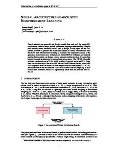
with an initial condition v(0) = (0, . . . , 0) ∈ Rn . Let us make a couple of observations about ODE (2). Figure 1 describes a typical illustration of the vectors that appear in this ODE for n = 2. The shaded area shows the acceptance set A(t), whose barycenter with / ∫ ∫ respect to the probability measure µ is A(t) xdµ µ(A(t)). Therefore the term λ A(t) (x − v(t))dµ is parallel to the vector from v(t) to the barycenter of A(t), which represents the gain upon agreement. On the other hand, −ρv(t) captures the loss from discounting. 9

x2 barycenter of A(t)

A(t) X

v(t) −ρv(t)

v (t) ′

λ

R

A(t) (x

− v(t))dµ

x1

v(0) = 0

Figure 1: Vectors in ODE (2) Velocity vector v ′ (t) is the sum of these two vectors. The absolute value of the integral on the right hand side of (2) is proportional to the weight µ(A(t)). If ρ = 0, (2) immediately implies vi′ (t) ≥ 0 for all t and i ∈ N , and vi′ (t) = 0 if and only if µ(A(t)) = 0. Now we see that a standard argument of ordinary diﬀerential equations shows that ODE (2) has a solution whenever Assumption 1 holds.12 The cutoﬀ strategy proﬁle with a cutoﬀ proﬁle given by this solution of ODE (2) turns out to be a trembling-hand equilibrium, as shown in the following proposition. Proposition 2. There exists a trembling-hand equilibrium that consists of (Markov) cutoﬀ strategies. By Proposition 1, the solution of ODE (2) is unique. Therefore the game has essentially a unique trembling-hand equilibrium for any given X and µ. Let us denote the unique solution of (2) by v ∗ (t; ρ, λ), the continuation payoﬀ proﬁle in the trembling-hand equilibrium. We simply denote this by v ∗ (t) as long as there is no room for confusion. To prepare for the main sections in which we investigate the asymptotic behavior of v ∗ (t) as the arrival rate λ becomes large, we show a useful lemma which is directly derived from the form of ODE (2). Lemma 3. For any α > 0, v ∗ (t; ρ, αλ) = v ∗ (αt; ρ/α, λ) if −t, −αt ∈ [−T, 0]. Next we note that, under certain assumptions, v ∗ (t; ρ, λ) converges to an allocation v ∗ independent of t in the limit of λ → ∞. This convergence is obvious if ρ = 0. ˆ is compact, limT →∞ v ∗ (T ; 0, λ) clearly exists. Since v ′ (t) is always nonnegative and X Since v ∗ (T ; 0, λ) = v ∗ (λT ; 0, 1) by Lemma 3, v ∗ = limλ→∞ v ∗ (T ; 0, λ) also exists, and is ˆ is compact. See Coddington This is because the right hand side of ODE (2) is continuous in v, and X and Levinson (1955, Chapter 1) for a general discussion about ODE. 12

10

x2 X

v∗

barycenter of A(t)

A(t)

v(t) v ′ (t)

x1

v(0) = 0

Figure 2: The path and the velocity vector of ODE (3) independent of T . If ρ > 0, the existence of v ∗ = limλ→∞ v ∗ (t) is not straightforward since vi′ (t) may be negative. We postpone a proof of the existence of this limit in the case of positive ρ until Proposition 12 in Section 5. In the following two sections, we analyze the limit of the continuation payoﬀs in the equilibrium and the expected duration that the search process continues, as the frequency of Poisson arrival goes to inﬁnity. This limit is considered in two cases: the case when the payoﬀs realize at the deadline (Section 4), and the case when the payoﬀs realize as soon as the agreement is reached (Section 5).

4

Asymptotic Results when the Payoﬀs Realize at the Deadline

In this section, we consider the case in which players receive beneﬁts of the agreement only at the deadline even when they stop searching earlier. Mathematically, this is equivalent to analyzing the limit of the continuation payoﬀ proﬁle limλ→∞ v ∗ (t) in the equilibrium when ρ = 0. In this case, v ∗ (t) is characterized as the unique solution of the following ordinary diﬀerential equation given by letting ρ = 0 in ODE (2): ′

∫

(

v (t) = λ

) x − v(t) dµ

(3)

A(t)

with an initial condition v(0) = (0, . . . , 0) ∈ Rn . Figure 2 describes a path of the solution ∫ of ODE (3) for n = 2. At time −t ∈ [−T, 0], the velocity vector v ′ (t) equals λ A(t) (x − v(t))dµ, which is parallel to the vector from v(t) to the barycenter of A(t) weighted by µ. 11

x2 1

X

v∗

1/2 v(t) v(0) = 0

X 1/2

1

x1

Figure 3: A path that converges to a weakly Pareto eﬃcient allocation. We present asymptotic results of the continuation payoﬀs v ∗ (t) as the arrival rate λ tends to inﬁnity. If λ is very large, one may conjecture that players have so many opportunities that they can ﬁnd a good allocation. We discuss eﬃciency of the limit v ∗ = limλ→∞ v ∗ (t; 0, λ) in X to show that this intuition is basically correct. Let us note that we sometimes consider the limit limt→∞ v ∗ (t; 0, λ) with enlarging the time interval [−T, 0]. By Lemma 3, v ∗ = limt→∞ v ∗ (t; 0, λ) for all λ. This implies that we can consider the two limits interchangeably; the limit of v ∗ (t) as t → ∞, and the limit as λ → ∞ for ﬁxed t. In general, v ∗ is not necessarily Pareto eﬃcient in X. There is an example of a probability density function f satisfying Assumption 1 in which v ∗ (t) converges to an allocation that is not strictly Pareto eﬃcient. ( ) ( ) Example 1. Let n = 2, X = [0, 1/2]×[3/4, 1] ∪ [3/4, 1]×[0, 1/2] , and f be the uniform density function on X, which is shown in Figure 3. By the symmetry with respect to the 45 degree line, we must have v1∗ (t) = v2∗ (t) for all t. Therefore v ∗ = (1/2, 1/2), which is not Pareto eﬃcient in X. Note that v ∗ is weakly Pareto eﬃcient, and that X is a non-convex set in this example. In fact, we will show that v ∗ is always weakly eﬃcient for general X, and strictly Pareto eﬃcient if X is convex. Furthermore, even if X is not convex, we can show v ∗ is “generically” Pareto eﬃcient, that is, v ∗ is Pareto eﬃcient in X for any generic f that satisﬁes Assumption 1. ˆ = {v ∈ Rn | x ≥ v for some x ∈ X} is the positive region of the Remember X + comprehensive extension of X. Lemma 4. The solution v ∗ (t) of equation (3) converges to a weakly Pareto eﬃcient ˆ as λ → ∞. allocation in X

12

Let F be the set of density functions that satisfy Assumption 1. We consider a topology on F deﬁned by the following distance in F: For f, f˜ ∈ F , f − f˜ = sup f (x) − f˜(x) . x∈X

Proposition 5. The set {f ∈ F | v ∗ is Pareto eﬃcient in X} is open and dense in F. This proposition shows that v ∗ is eﬃcient only for generic f . However, if X is convex, then v ∗ is eﬃcient for all f . Proposition 6. Suppose that X is a convex set. Then v ∗ is Pareto eﬃcient in X. Weak Pareto eﬃciency leads to an observation that players reach an agreement almost surely if t is very large. Let p(t) be the probability that players reach an agreement in the equilibrium before the deadline given no agreement at time −t. Then the continuation ˆ which implies v ∗ (t)/p(t) ∈ X. ˆ We payoﬀs v ∗ (t) must fall in the set {p(t)v | v ∈ X}, have vi∗ (t) > 0 for all t > 0 and i ∈ N since vi∗ (t) is nondecreasing and vi∗′ (0) > 0 by equation 3. Since there is a positive probability that no opportunity arrives before the ˆ strictly Pareto dominates deadline, p(t) is smaller than one. Therefore v ∗ (t)/p(t) ∈ X ˆ v ∗ (t). This implies limt→∞ p(t) = 1 since by Lemma 4 v ∗ is weakly Pareto eﬃcient in X. Now we show the following proposition: Proposition 7. The probability of agreement before the deadline converges to one as the time interval becomes large. In Propositions 5 and 6, we showed that v ∗ (t) almost always converges to the Pareto frontier of X. We consider the inverse problem. For any Pareto eﬃcient allocation w in X which is not at the edge of the Pareto frontier,13 we show that one can ﬁnd density f which satisﬁes Assumption 1 such that the limit of the solution v ∗ (t) of equation (3) is w. Proposition 8. Suppose that w is a Pareto eﬃcient allocation in X such that wi > 0 for all i ∈ N , and w is not located at the edge of the Pareto frontier. Then there exists a probability measure µ satisfying Assumption 1 such that the equilibrium continuation payoﬀ proﬁle v ∗ (t) converges to w as λ tends to inﬁnity. In the proof, we construct a probability density function f to have a large weight near w ∈ X, and show that the limit continuation payoﬀs is w if there is a suﬃciently large 13

We formally deﬁne this property in the proof given in Appendix A.8.

13

weight near w. Note that this claim is not so obvious as it seems. Indeed, we will see in Section 5 that the limit is independent of density f if there is a positive discount rate ρ > 0, as long as Assumption 1 holds. In the rest of this section, we make assumptions on regularity of X around v ∗ in addition to Assumption 1. Assumption 2. (a) The limit v ∗ is Pareto eﬃcient in X. (b) The Pareto frontier of X is smooth in a neighborhood of v ∗ . (c) For the unit normal vector α ∈ Rn+ at v ∗ , αi > 0 for all i ∈ N . (d) For all η > 0, there exists ε > 0 such that {x ∈ Rn+ | |v ∗ − x| ≤ ε, α · (x − v ∗ ) ≤ −η} is contained in X, where “·” denotes the inner product in Rn .14 The next lemma shows that v ∗ (t) converges to v ∗ with a speed of order (λt)−1/n . Lemma 9. Suppose that Assumption 2 holds. As either t → ∞ or λ → ∞, (vi∗ − vi∗ (t))(λt)1/n converges to a positive and ﬁnite value which is written as lim (vi∗ t→∞

−

1 vi∗ (t))(λt) n

(

n + 1 ∏ αj ) n1 = f (v ∗ )nn+1 j̸=i αi

for all i ∈ N , where α ∈ Rn++ be the unit normal vector of X at v ∗ . In the present model with ﬁnite λ, it always takes positive time for players to reach an agreement. The next proposition shows that if the Pareto frontier of X is smooth and v ∗ (t) converges to the Pareto frontier, then the expected duration of the search process in the time interval [−T, 0] is (n2 T )/(n2 + n + 1). Proposition 10. Suppose that Assumption 2 holds. Then the expected duration of search n2 in the equilibrium is 2 T. n +n+1 The proposition implies that a positive fraction of time is spent on search, but players do not spend all the time they have. This is a result of a tradeoﬀ between two eﬀects: On one hand, players do not want to wait too much, as doing so would result in disagreement, or the agreement in low payoﬀs which they would receive if it takes place close to the deadline. On the other hand, players do not want to stop their search immediately, as they are very picky when the deadline is very far away. Being picky is optimal for the players, as there is no discounting. In the next section, we will see that if there is a signiﬁcant eﬀect of discounting we expect the search to end immediately. Putting it another way, there are two eﬀects of making the arrival rates large. One is that there exist many realizations of payoﬀs in a given time interval, which makes the possibility of 14

Only condition (b) is necessary if X is convex.

14

Number of agents

1

2

3

5

10

100

Limit expected duration .33 .57 .69 .81 .90

.99

Table 1: Limit expected duration of search as opportunities arrive more and more frequently.

Prob. of agreement 1 .86 λ→∞ λ=1 0

−10

time

Figure 4: A numerical example of the cumulative probability of agreement. agreement more likely. The other is that as the result of the increase of opportunities, players expect more opportunities in the future, which makes them pickier. The solution of the expected duration provided in the theorem implies that, if only two players are involved in search, the expected duration is 47 T , it monotonically increases to approach T as n gets larger. Table 1 shows the limit expected duration for several n’s when T = 1.15 We do not think the reason for this is a simple one, which would say that if there are many people it is diﬃcult to all agree on something. The result is rather the consequence of two distinct eﬀects explained above. The limit duration of Proposition 9 is not far away from those with ﬁnite λ in many cases. In the apartment search example, let us suppose that the couple has ten weeks before the deadline, and a broker provides information of an apartment once in every week on average. Figure 4 shows a graph of the cumulative probability of agreement for λ = 1 and λ → ∞ when T = 10, N = {1, 2}, X = {(x1 , x2 ) ∈ R2+ | x1 + x2 ≤ 1}, and µ is the uniform distribution on X. The probability of agreement before any time −t does not change more than 15% if one considers quite a frequent search instead of searching once a week. A straightforward computation shows that the expected duration of search is decreasing in λ, and it is 6.08 for λ = 1, which is only 6.5% longer than the limit expected duration (4/7) · 10 = 5.71.

Although we assumed n ≥ 2, one can easily show that the same analysis applies to the search problem with a single agent. 15

15

5

Asymptotic Results when the Payoﬀs Realize upon Agreement

In this section, we consider the limit of the equilibrium continuation payoﬀs v ∗ (t) as λ → ∞ when the payoﬀs realize as soon as an agreement is reached. First, we note that if ρ = 0, exactly the same analysis as in the previous section applies, as we have already discussed. Hereafter we consider the case where ρ > 0. Let us revisit the ordinary diﬀerential equation (2) that characterizes the equilibrium continuation payoﬀ proﬁle v ∗ (t) as its unique solution: ∫

′

v (t) = −ρv(t) + λ

(

) x − v(t) dµ

(2)

A(t)

with an initial condition v(0) = (0, . . . , 0). If λ is large, the right hand side of equation (2) is approximated by the right hand side of equation (3). Therefore, v ∗ (t) is close to the solution of equation (3) in the case of ρ = 0, for λ large relative to ρ. This resemblance of trajectories holds until v ∗ (t) approaches the ˆ In particular, we can show that v ∗ (t) approaches v 0 arbitrarily closely boundary of X. as λ → ∞, where v 0 is deﬁned as the limit of the solution of equation (3). Note that v 0 is weakly Pareto eﬃcient by Lemma 4. ¯ > 0 such that for all λ ≥ λ, ¯ Proposition 11. For all ε > 0, there exists λ 0 v − v ∗ (t) ≤ ε for some t. Remark 1. Before analyzing v ∗ = limλ→∞ v ∗ (t; ρ, λ), let us consider another limit v ∗ (∞; ρ, λ) = limt→∞ v ∗ (t; ρ, λ). Since the right hand side of equation (2) is not proportional to λ, these two limits do not coincide for positive ρ > 0. If the limit v ∗ (∞) exists, this must satisfy ∫ ( ) ∗ ρv (∞) = λ x − v ∗ (∞) dµ (4) A ∗

where A = {x ∈ X | x ≥ v (∞)}. For ρ > 0, equality (4) shows µ(A) > 0, which follows that v ∗ (∞) is Pareto ineﬃcient in X. This will contrast eﬃciency of v ∗ = limλ→∞ v ∗ (t; ρ, λ) shown in Proposition 12. Equality (4) also implies that v ∗ (∞) is parallel to the vector from v ∗ (∞) to the barycenter of A, as shown in Figure 5 in the two-dimensional case. We assume the following simplifying conditions until the end of this section.16 Assumption 3. The Pareto frontier of X is smooth, and every component of the normal vector at any Pareto eﬃcient allocation in X is strictly positive. 16

We can show basically the same results without this assumption. We avoid complications derived from the indeterminacy of a normal vector on the boundary of X.

16

A barycenter of A

barycenter of Pareto frontier of A

v ∗ (∞) λ −ρv ∗ (∞)

R

A (x

− v ∗ (∞))dµ

(0, 0)

Figure 5: Vectors when t → ∞. Now suppose that λ is very large. Then µ(A) must be very small, which means that v (∞) is very close to the Pareto frontier of X. By Assumption 1, the density f is approximately uniform in A if A is a set with a very small area. To obtain an intuition, suppose that A is a small n-dimensional pyramid. The vector in the right hand side of equality (4) is parallel to the vector from v ∗ (∞) to the barycenter of the Pareto frontier of A. If x is the barycenter of the Pareto frontier of A, it turns out that the boundary of ∏ A at x is tangent to the hypersurface deﬁned by i∈N xi = a for some constant a. We refer to such a Pareto eﬃcient allocation as a Nash point, and the set of all Nash points as the Nash set of (X, 0) (Maschler et al. (1988), Herrero (1989)). The Nash set contains all local maximizers and all local minimizers of the Nash product. If X is convex, there exists a unique Nash point, which is called the Nash bargaining solution. The above observation leads to the next proposition. ∗

Proposition 12. Suppose that any Nash point is isolated in X. Then the limit v ∗ = limλ→∞ v ∗ (t) exists and belongs to the Nash set of the problem (X, 0). In particular, if X is convex, this limit coincides with the Nash bargaining solution of (X, 0). Therefore, the trajectory of v ∗ (t) for very large λ starts at v ∗ (t) = 0, approaches v 0 , and moves along the Pareto frontier until reaching a point close to a Nash point. Finally we consider the duration of search in the equilibrium. In contrast to Proposition 10 in the case of ρ = 0, we show that players reach an agreement almost immediately if λ is very large. ¯ > 0 such that the Proposition 13. For all −t ∈ (−T, 0] and all ε > 0, there exists λ probability that players reach an agreement before time −t in the equilibrium is larger ¯ than 1 − ε for all λ ≥ λ.

17

x2 1

X

ρ=0

v0 ( 21 , 12 )

ρ>0

v(0) = 0

1

x1

Figure 6: Paths of continuation payoﬀs. The probability density is low near (1, 0), and high near (0, 1).

6 6.1

Discussion Dynamics of Bargaining Powers

Consider the case where X = {x ∈ R2+ | x1 + x2 ≤ 1} and a density f such that f (x) > f (x′ ) if x2 −x1 > x′2 −x′1 . Suppose ρ > 0 is very small. In this case, the limit of the solution of ODE (3) with ρ = 0, denoted v 0 , locates at the boundary of X by Proposition 6, and it is to the north-west of ( 21 , 21 ), which is the Nash bargaining solution and is the limit of the solution of ODE (2). Hence, by Proposition 11, the continuation payoﬀ when the players receive payoﬀs upon the agreement starts at a point close to ( 12 , 12 ), and goes up along the boundary of X and reaches a point close to v 0 , and then goes down to (0, 0). On this path of play, player 1’s expected payoﬀ is monotonically decreasing over time. On the other hand, player 2’s expected payoﬀ changes non-monotonically. Speciﬁcally, it rises up until it reaches close to v20 , and then decreases over time. Figure 6 illustrates this path. Underlying this non-monotonicity is the change in bargaining power between the players. When the deadline is far away, there will be a lot of opportunities left until the deadline, so it is unlikely that players will accept allocations that are far from the Pareto eﬃcient allocations, so the probability distribution over such allocations does not matter so much. Since X is convex and symmetric, two players expect roughly the same payoﬀs. However, as the time passes, the deadline comes closer, so players expect more possibility that Pareto-ineﬃcient allocations will be accepted. Since player 2 expects more realizations favorable to her than player 1 does, player 2’s expected payoﬀ rises while player 1’s goes down. Finally, as the deadline comes even closer, player 2 starts fearing the possibility of reaching no agreement, so she becomes less pickier and the cutoﬀ goes down accordingly.

18

6.2

Simultaneous Convergence

In Section 4, we have shown that if ρ = 0, the limit equilibrium payoﬀs as λ → ∞ are eﬃcient but dependent on the distribution µ. In Section 5, in contrast, the limit is the Nash bargaining solution if ρ > 0 is ﬁxed. In this section, we show that the limit equilibrium payoﬀs as λ → ∞ and ρ → 0 simultaneously depends on where λρn converges to. Proposition 14. Suppose that Assumptions 2 and 3 hold. The limit v ∗ = limλ→∞,ρ→0 v ∗ (t; ρ, λ) satisﬁes the following claims: (i) If λρn → 0, then v ∗ = limλ→∞ v ∗ (t; 0, λ), which is the limit analyzed in Section 4, and (ii) if λρn → ∞, then v ∗ = limλ→∞ v ∗ (t; ρ, λ) for ρ > 0, which is the limit shown in Section 5. An insight behind this result is as follows: The limit depends on whether the ﬁrst term in ODE (2) is negligible or not when compared to the second term. Let z(t; ρ, λ) be the Hausdorﬀ distance from v ∗ (t; ρ, λ) to the Pareto frontier of X. If ρ is very small and λ is not very large, Proposition 11 shows that v ∗ (t; ρ, λ) is close to limλ→∞ v ∗ (t; 0, λ) which is on the Pareto frontier. Then we can apply Lemma 9 to show that z(t; ρ, λ) is approximately proportional to λ−1/n . Since µ(A(t)) approximates z(t; ρ, λ)n (times some constant), and the length of the vector from v ∗ (t; ρ, λ) to the barycenter of A(t) is linear in z(t; ρ, λ), the second term is of order λ · λ−1/n · λ−1 = λ−1/n . Therefore if λρn → 0 the ﬁrst term, which approximates ρv ∗ , is negligible because ρ vanishes more rapidly than λ−1/n . If λρn → ∞, the ﬁrst term is signiﬁcant because ρ does not vanish rapidly compared to λ−1/n . Remark 2. Gomes et al. (1999) consider a discrete-time ﬁnite-horizon n-player bargaining with a general coalitional form. A proposer is selected with equal probability in every period, and if her proposal is rejected, she drops out of bargaining with a small probability. They investigate the limit subgame perfect equilibrium payoﬀ proﬁle as the probability of breakdown vanishes and the horizon length tends to inﬁnity. The limit is shown to be the Raiﬀa solution (deﬁned appropriately in the setting of a general coalitional form) if the speed that the probability of breakdown vanishes is suﬃciently faster than the speed that the horizon length goes to inﬁnity, and it is the Nash solution (or more general concept of the NTU consistent value) if the latter is suﬃciently faster than the former. Imai and Salonen (2009) consider a related two-player model. They analyze a limit solution as the number of periods in the ﬁxed length of horizon becomes large. This solution turns out to be between the Raiﬀa and the Nash solution, which are borderline cases of Gomes et al. (1999). Despite common features such as presence of deadline, and analysis of limits in multiple cases, the present paper diﬀers from these works in the following three aspects. First, proposers in the above bargaining model have a full control of their proposals. In 19

a subgame perfect equilibrium, players reach an agreement immediately because a proposer always oﬀers an allocation accepted by the others given continuation payoﬀs in subsequent subgames. On the other hand, realization of an allocation at each moment is stochastic in our model, hence it is not ex ante obvious whether the duration of search shrinks as we let the arrival rate go to inﬁnity. Indeed, we have shown in Proposition 10 that when the payoﬀs realize at the deadline, players spend a signiﬁcant amount of time for search. Second, the conditions that determines whether the limit equilibrium payoﬀs is Nash solution or not are diﬀerent. In the bargaining models, the condition is expressed by the limit of the probability that there is no breakdown in the entire bargaining conditional on no agreement at all (Gomes et al. (1999, Theorem 4.4)). Since imposing a breakdown with probability π at an opportunity is mathematically equivalent to discounting payoﬀs with discount factor 1−π, and there are λ opportunities in average in a unit time interval in the Poisson process, the discount rate ρ is given by e−ρ = (1 − π)λ . Therefore the probability of no breakdown corresponds to (1−π)λT = e−ρT which does not depend on λ. This contrasts our Proposition 14, in which the term in the convergence condition depends on λ. This distinction derives from the diﬀerence in the probabilities of agreement at an opportunity on the equilibrium path. In our search model, the probability of realization falling into the acceptance set is the nth order of the distance to the limit payoﬀ proﬁle, while players reach an agreement with probability one in the bargaining model. Third, the processes by which opportunities arrive diﬀer in two models. In Gomes et al. (1999) and Imai and Salonen (2009), players have an opportunity for sure in every ﬁxed time interval. This implies that there is the “last period” (unless a breakdown occurs). In contrast, our model have a positive probability that there comes no opportunity after any time −t. This distinction aﬀects the limit as λ → ∞. Let the discount rate be positive. Then, the limit payoﬀs in Imai and Salonen (2009) comes between the Raiﬀa and the Nash bargaining solutions as the number of periods in the ﬁxed length of horizon becomes large, whereas the limit in our search model is exactly the Nash bargaining solution independent of the level of discount rate ρ > 0. If there is the last period, players expect to obtain positive payoﬀs at the last period for sure. This eﬀect does not disappear in backward induction unless the time horizon goes to inﬁnity.

6.3

Inﬁnite-Horizon and Static Games

Although we consider a ﬁnite-horizon model, our convergence result in Proposition 12 is suggestive of that in inﬁnite-horizon models such as Wilson (2001), Compte and Jehiel (2010), and Cho and Matsui (2011), all of whom consider the limit as the discount factor goes to one in discrete-time inﬁnite-horizon models. This is because the threatening power of disagreement at the deadline is quite weak if the horizon is very far away, and

20

thus the inﬁnite-horizon model is similar to a ﬁnite-horizon model with T → ∞ if ρ > 0. In fact, we can show that the iterated limit as T → ∞ and then ρ → 0 is the Nash bargaining solution in our model. By Proposition 14, limρ→0 v ∗ (T ; αρ, αλ) with α = ρ−a is the Nash bargaining solution for all a > n/(n + 1). As a → ∞, we see that the iterated limit limρ→0 limα→∞ v ∗ (T ; αρ, αλ) is also the Nash bargaining solution. Since Lemma 3 shows that enlarging T is equivalent to rising λ and ρ in the same ratio, the iterated limit as T → ∞ ﬁrst and then ρ → 0 must be the Nash bargaining solution. Propositions 1 and 2 imply that the limit continuation payoﬀ is essentially equal to the cutoﬀ, which is expressed by a single variable. In this sense, there is some connection between our model and a static game considered by Nash (1953) himself, who provided a characterization of the Nash bargaining solution by introducing a static demand game with perturbation described as follows.17 Suppose that X is convex. The basic demand game is a one-shot strategic-form game in which each player i calls a demand xi ∈ R+ . Players obtain x = (x1 , . . . , xn ) if x ∈ X, or 0 otherwise. In the perturbed demand game, players fail to obtain x ∈ X with a positive probability if x is close to the Pareto frontier. Under certain conditions, he showed that the Nash equilibrium of the perturbed demand game converges to the Nash bargaining solution as the perturbation vanishes. Let us compare the perturbed Nash demand game with our multi-agent search model ( ) with a positive discount rate. Let p(x) = µ A(x) be the probability that players come across an allocation which Pareto dominates or equals x ∈ X at an opportunity. If T is very large and t is close to T , players at time −t choose almost the same cutoﬀ proﬁle, say x, contained in the interior of X. The average duration that players wait for an allocation falling into A(x) is almost 1/λp(x). During this time interval, payoﬀs are discounted at rate ρ. Since xi must be equal to her continuation payoﬀ in an equilibrium, i would lose nearly (1 − e−ρ/λp(x) )yi on average by insisting cutoﬀ xi where y is the expected allocation conditional on y ∈ A(x). Note that this loss vanishes as ρ → 0 for every x in the interior of X. Let probability P (y) satisfy P (y) = e−ρ/λp(x) . Player i loses the same expected payoﬀ when y ∈ X is demanded in the perturbed demand game where the probability of successful agreement is P (y). The key tradeoﬀ in this game, the attraction to larger demands or the fear of failure of agreement, is parallel to that in the multi-agent search, to be pickier or to avoid loss from discounting.

7

Conclusion

We investigated an n-person search problem with deadline in which agreement opportunities arrive according to the Poisson process, and the drawn object is adopted by a 17

We here follow a slightly modiﬁed game considered by Osborne and Rubinstein (1990, Section 4.3). Despite the diﬀerence, the model conveys the same insight as the original.

21

unanimous acceptance. If players cannot reach any agreement before the deadline, they obtain a predetermined payoﬀ proﬁle. We analyzed the limit of the equilibrium continuation payoﬀs as objects are drawn more and more frequently. If players receive payoﬀs at the deadline, the continuation payoﬀs are eﬃcient but sensitive to the distribution of the payoﬀs of the object in search. The limit expected duration of search is longer than a half of the length of the given time interval, increases in n, and converges to one as n goes to inﬁnity. On the other hand, if players receive payoﬀs immediately after they agree, the continuation payoﬀ proﬁle converges to a Nash point, and the duration of search is zero in the limit. We are currently working on several extensions and further investigation of our model. First, we have assumed that the disagreement payoﬀ is 0. This assumption is not entirely innocuous in the presence of discounting, but we expect none of our results change substantially even if we relax this assumption. Second, we have assumed that the discount rate is homogeneous across all the players. Allowing for heterogeneous discount rates will change the Nash bargaining solution to weighted Nash bargaining solution when the payoﬀs realize upon agreement, but the duration of search will not change. Third, our results pertain to the limit case as the arrival rates go to inﬁnity. We are exploring the case of ﬁnite arrival rates to conduct comparative statics exercises. We will address these and other points in our future research.

Appendix A.1

More Deﬁnitions

First we introduce deﬁnitions and notations used in proofs. Let xi = max{xi | (xi , x−i ) ∈ X for some x−i } be the maximum payoﬀ attainable for player i in X, fH = maxx∈X f (x) < ∞ be the upper bound, and fL = minx∈X f (x) > 0 be the lower bound of f in X. Note that Assumption 1 ensures existence of these values.

A.2

Proof of Proposition 1

Suppose that there exists at least one trembling-hand equilibrium. We show that the continuation payoﬀ of player i at time −t is unique in any trembling-hand equilibrium. Let v εi (t) and v εi (t) be the supremum and the inﬁmum of the set of continuation payoﬀs ˜ t \ Ht at time −t in all Nash equilibria σ in ui (σ | h) of player i after all histories h ∈ H the ε-constrained game. Let wiε (t) = v i (t) − v i (t), w ¯ ε (t) = maxi∈N wiε (t). We will show that w¯ ε (t) = 0 for all ε > 0 for any time −t ∈ [−T, 0]. Note that w ¯ ε (0) = 0 for all ε. Let us consider the ε-constrained game. If player i accepts an allocation x ∈ X at time −t, she will obtain xi with probability at least εn−1 . Accepting x is a dominant

22

action of player i if the following inequality holds: εn−1 xi + (1 − εn−1 )v εi (t) > v εi (t), which implies, xi > v εi (t) +

1 − εn−1 ε wi (t). εn−1

n−1

1 wiε (t). Then v˜iε (t) − v εi (t) = εn−1 wiε (t). Let v˜iε (t) = v εi (t) + 1−ε εn−1 Let Xi1 (t) = {x ∈ X | xi ≥ v˜iε (t)}, Xim (t) = {x ∈ X | v εi (t) ≤ xi ≤ v˜iε (t)}, and Xi0 (t) = {x ∈ X | xi ≤ v εi (t)}. Any player i accepts x ∈ Xi1 (t) and rejects x ∈ Xi0 (t) with (∪ ) m probability 1 − ε after almost all histories at time −t. Note that X = j∈N Xj (t) ∪ ) (∪ ∩ sj (s1 ,...,sn )∈{0,1}n j∈N Xj (t) (although not disjoint). Then

v εi (t)

≤

∫ t (∑ ∫ 0

j∈N

Xjm (τ )

∑

+

xi dµ ∫

(

∩ (s1 ,...,sn

)∈{0,1}n

sj j∈N Xj (τ )

∑

+ (1 − (1 − ε)

j∈N

sj

ε

∑

∑

(1 − ε)

j∈N (1−sj )

j∈N

sj

∑

ε

j∈N (1−sj )

xi

) ) )v εi (τ ) dµ λe−(λ+ρ)(t−τ ) dτ ,

and v εi (t)

≥

∫ t( 0

∑

∫

( ∩

(s1 ,...,sn )∈{0,1}n ∑

+ (1 − (1 − ε)

sj j∈N Xj (τ )

j∈N

sj

ε

∑

(1 − ε)

j∈N (1−sj )

23

∑ j∈N

)

)v εi (τ )

sj

ε

)

∑

j∈N (1−sj )

xi

dµ λe−(λ+ρ)(t−τ ) dτ .

Therefore wiε (t) = v i (t) − v i (t) is estimated as follows: wiε (t)

≤

∫ t (∑ ∫ 0

j∈N

xi dµ

Xjm (τ )

∫

∑

+

∩ (s1 ,...,sn )∈{0,1}n

≤

∫ t (∑ 0

fH xi

j∈N

0

+

j∈N

Xj j (τ )

1

ε

wε (τ ) n−1 j ∫

∑ j∈N

sj

ε

∑

j∈N (1−sj )

(

)

) wiε (τ )dµ λe−(λ+ρ)(t−τ ) dτ

xk

k̸=j ∑

1 − (1 − ε)

fH max{xk } k∈N

∑

∏

1 − (1 − ε)

j∈N

sj

∑

ε

j∈N (1−sj )

)

) wiε (τ )dµ λe−(λ+ρ)(t−τ ) dτ

X

(s1 ,...,sn )∈{0,1}n

∫ t (∑

s

j∈N

∑

+ ≤

(

(

1 ∏ εn−1

xk

k̸=j ∑

1 − (1 − ε)

j∈N

sj

∑

ε

j∈N (1−sj )

))

wε (τ )λe−(λ+ρ)(t−τ ) dτ .

(s1 ,...,sn )∈{0,1}n

Since the above inequality holds for all i ∈ N , there exists a constant L > 0 such that the following inequality holds: ∫

t

w (t) ≤ ε

Lwε (τ )e−(λ+ρ)(t−τ ) dτ .

0

Let W ε (t) =

∫t 0

wε (τ )e(λ+ρ)τ dτ . Then W ε′ (t) = wε (t)e(λ+ρ)t ≤ W ε (t).

( ) Therefore we have dtd W ε (t)e−t ≤ 0, which implies wε (t) ≤ W ε (t) ≤ 0 since wε (0) = 0. Hence, wε (t) = 0 for all t and all ε > 0. Any trembling-hand equilibria yield the same continuation payoﬀs after almost all histories at time −t ∈ [−T, 0].

A.3

Proof of Proposition 2

We show that the unique solution v ∗ (t) of ODE (2) characterizes a trembling-hand equilibrium. For si ∈ {+, −}, and vi ∈ [0, xi ] let  [0, v ] if s = +, i i Iisi (vi ) = [v , x ] if s = −, i i i

24

and p+ = 1 − ε, p− = ε. For ε > 0, let us write down a Bellman equation similar to (1) with respect to a continuation payoﬀ proﬁle v ε (t) in the ε-constrained game: viε (t)

=

∫ t( ∑ 0

∫

( s

s∈{+,−}n

(I1 1 (viε (τ ))×···×Insn (viε (τ )))∩X

) ) ps1 . . . psn · xi + (1 − ps1 . . . psn )viε (τ ) dµ

· λe−(λ+ρ)(t−τ ) dτ This implies that viε′ (t) = −(λ + ρ)viε (t) ∑ ∫ +λ s∈{+,−}n

( s

(I1 1 (viε (t))×···×Insn (viε (t)))∩X

) ps1 . . . psn · xi + (1 − ps1 . . . psn )viε (t) dµ.

This ODE has a unique solution because the right hand side is uniformly Lipschitz continuous in viε . Let v ε (t) be this solution, which is a cutoﬀ proﬁle of a Nash equilibrium in the ε-constrained game by construction. Since A(t) = (I1+ (viε (τ )) × · · · × In+ (viε (τ ))) ∩ X, and p+ → 1, p− → 0 as ε → 0, ODE 2 is obtained by letting ε → 0. Therefore v ε (t) converges to v ∗ (t) as ε → 0 because the above ODE is continuous in ε.18 Hence the cutoﬀ strategy proﬁle with cutoﬀs v ∗ (t) is a trembling-hand equilibrium.

A.4

Proof of Lemma 3

Let w∗ (t; ρ, λ) = v ∗ (αt; ρ/α, λ). By equation (3), w∗ (t; ρ, λ) is the solution of ρ w (t/α) = − w(t/α) + λ α ′

∫

(

) x − w(t/α) dµ,

A(w(t/α))

which is equivalent to d w(τ ) = −ρw(τ ) + αλ dτ

∫

(

) x − w(τ ) dµ

A(w(τ ))

where τ = t/α, w(t) = v(αt). The solution of the second equation is w∗ (t; λ) = v ∗ (t; αλ). Therefore we have v ∗ (t; ρ, αλ) = v ∗ (αt; ρ/α, λ) as desired.

A.5

Proof of Lemma 4

By Lemma 3, it suﬃces to show that v ∗ = limt→∞ v ∗ (t) is weak Pareto eﬃcient. Let A = {x ∈ X | x ≥ v ∗ }. Suppose that there exists x = (x1 , . . . , xn ) ∈ A such that x1 > v1∗ , . . . , xn > vn∗ . By Assumption 1, there exists a closed subset Y ⊂ A such 18

See, e.g., Coddington and Levinson (1955, Theorem 7.4 in Chapter 1).

25

µ(Y ) > 0, and yi = inf{xi | (x1 , . . . , xn ) ∈ Y } > xi . By ODE (3), we have vi∗′ (t)

∫

(

=λ

) xi − vi∗ (t) dµ

A(t)

∫ ≥λ

(yi − vi∗ )dµ

W

= λ(yi − vi∗ )µ(Y ) > 0. This inequality implies that vi∗ (t) ≥ λ(yi − vi∗ )µ(Y )t + vi∗ (0), which tends to inﬁnity as t → ∞. This contradicts the fact that vi∗ (t) is convergent. Hence x is weakly Pareto ˆ eﬃcient in X.

A.6

Proof of Proposition 5

Let v ∗ (t; f ) be the solution of ODE (3) for density f ∈ F , and v ∗ (f ) = limλ→∞ v ∗ (t; f ) = limt→∞ v ∗ (t; f ). First we show that the set is open, i.e., for all f ∈ F with v ∗ (f ) Pareto eﬃcient, ε > 0, and a sequence fk ∈ F (k = 1, 2, . . . ) with |fk − f | → 0 (k → ∞), there exist δ > 0 and k¯ such that |v ∗ (fk ) − v ∗ (f )| ≤ ε ¯ for all k ≥ k. Since limt→∞ v ∗ (t; f ) = v ∗ (f ), for all δ > 0 there exists t¯ > 0 such that |v ∗ (f ) − v ∗ (t; f )| ≤ δ for all t ≥ t¯. By Pareto eﬃciency of v ∗ (f ), let δ > 0 be suﬃciently small so ( ) that A v ∗ (t¯; f ) − (δ, δ, . . . , δ) is contained in the ε-ball centered at v ∗ (f ). Since the right hand side of ODE (3) is continuous in v, the unique solution of (3) is continuous with respect to parameters in (3). Therefore, for a ﬁnite time interval [0, T ] including t¯, there ¯ This implies that exists k¯ such that |v ∗ (t; fk )−v ∗ (t; f )| ≤ δ for all t ∈ [0, T ] and all k ≥ k. ( ) ( ) v ∗ (t; fk ) ∈ A v ∗ (t¯; f ) − (δ, δ, . . . , δ) , thereby v ∗ (fk ) ∈ A v ∗ (t¯; f ) − (δ, δ, . . . , δ) . Hence we have |v ∗ (fk ) − v ∗ (f )| ≤ ε. Second we show that the set is dense, i.e., for all f ∈ F with v ∗ (f ) not strictly Pareto eﬃcient in X and all ε > 0, there exists f˜ ∈ F such that |f − f˜| ≤ ε and v ∗ (f˜) is Pareto ˆ there exists Pareto eﬃcient eﬃcient. Since v ∗ (f ) is only weakly Pareto eﬃcient in X, y ∈ X which Pareto dominates v ∗ (f ). Let I = {i ∈ N | yi = vi∗ (f )} and J = N \ I. Since y is Pareto eﬃcient, there is δ > 0 such that if x ∈ X is weakly Pareto eﬃcient, satisﬁes |y − x| ≤ δ, and yi = xi for some i ∈ N , then there is no x˜ ∈ X such that x˜i > yi and |y − x˜| ≤ δ. By Assumption 1, for any small δ/2 > η > 0, there is a small ball contained in X centered at y˜ with |y − y˜| ≤ η. Let g be a continuous density function whose support is

26

the above small ball, takes zero on the boundary of the ball, and the expectation of g is ε ε exactly y˜. Let f˜ = (1 − |f |+|g| )f + |f |+|g| g ∈ F . Since f and g are bounded from above, |f − f˜| ≤ ε. ∪ ( Since v ∗ (f ) is weakly Pareto eﬃcient, if v ∗ (f ) ∈ A(v), then A(v) ⊂ i∈N [vi , vi∗ (f )] × ) ∏ ∗ j̸=i [0, xj ] . If |v (f ) − v| ≤ ξ where ξ > 0 is very small, ∫ (xi − vi )f (x)dx ≤ fH A(v)

∑

(vj∗ (f ) − vj )

j∈N

≤ ξnfH

∏

∏

xk

k∈N

xk

k∈N

If v ∗ (f ) ∈ A(v), minj∈N (yj − vj ) ≥ 2η and |v ∗ (f ) − v| ≤ ξ, we have ∫

∫

∫

(xi − vi )f˜(x)dx − A(v)

(xi − vi )(f˜(x) − f (x))dx A(v) ∫ ε = (xi − vi )(g(x) − f (x))dx |f | + |g| A(v) ( ( ∏ )) ε (˜ yi − vi ) − ξnfH ≥ xk . |f | + |g| k∈N

(xi − vi )f (x)dx = A(v)

If j ∈ J and |v ∗ (f ) − v| ≤ ξ where ξ > 0 is very small, then ∫

∫ (xj − vj )f˜(x)dx −

A(v)

(xj − vj )f (x)dx ≥ A(v)

ε (˜ yj − vj∗ (f )). 2(|f | + |g|)

Let w(t) = v ∗ (t; f˜) − v ∗ (t; f ). Since ODE (3) is continuous in the parameters, for all ζ > 0, there exists ε > 0 such that |w(t)| ≤ ζ for all t ∈ [0, T ]. Suppose that T and t are very large so that |v ∗ (f ) − v ∗ (t; f )| ≤ ξ. For j ∈ J, wj′ (t) is estimated as follows: wj′ (t)

∫ =λ A(v ∗ (t;f˜))

(xj −

vj∗ (t; f˜))f˜(x)dx

(xj −

vj∗ (t; f˜))f˜(x)dx

∫ =λ

A(v ∗ (t;f˜))

∫

+λ A(v ∗ (t;f˜))

(xj −

−λ

∫

A(v ∗ (t;f ))

(xj − vj∗ (t; f ))f (x)dx

∫ −λ

vj∗ (t; f˜))f (x)dx

λε (˜ yj − vj∗ (f )) − λ ≥ 2(|f | + |g|) ∫ −λ

A(vj∗ (t;f˜)))

(xj − vj∗ (t; f˜)))f (x)dx

∫

−λ

A(v ∗ (t;f ))

A(v ∗ (t;f ))∩A(v ∗ (t;f˜))

A(v ∗ (t;f ))\(A(v ∗ (t;f ))∩A(v ∗ (t;f˜)))

≥

∫

(xj − vj∗ (t; f ))f (x)dx

wj (t)f (x)dx

(xj − vj∗ (t; f ))f (x)dx

∑∏ ∏ λε (˜ yj − vj∗ (f ) − ζ) − λζξ xl − λξnfH xk . 2(|f | + |g|) k∈N l̸=k k∈N

27

Therefore when ξ > 0 is suﬃciently small, wj′ (t) is bounded away from zero: wj′ (t) ≥

λε (˜ yj − vj∗ (f ) − ζ). 4(|f | + |g|)

This implies that for small ε > 0 and large t, vj∗ (t; f˜) > v ∗ (f ) for all j ∈ J. Then the similar method to Step 3 in the proof of Proposition 6 shows that v ∗ (t; f˜) converges to a Pareto eﬃcient allocation in X.

A.7

Proof of Proposition 6

Let A = {x ∈ X | x ≥ v ∗ }. Let I = {i ∈ N | xi = vi for all x ∈ A} ⊂ N , and J = N \ I. Suppose that there exists x ∈ X which Pareto dominates v ∗ , thereby J ̸= ∅. Step 1: We show that I is nonempty. If there is no such player, there exist y(1), . . . , y(n) ∑ such that y(j) ∈ A and yj (j) > vj∗ for all j ∈ N . This implies that y = n1 j∈N y(j) strictly Pareto dominates v ∗ . Since X is convex, y also belongs to A. This contradicts the weak Pareto eﬃciency of v ∗ shown in Lemma 4. Step 2: Next we show that if v ∗ is not Pareto eﬃcient in X, and i ∈ I, then xi ≤ vi∗ for all x ∈ X. Let i be the player in I. Suppose that there exists y ∈ X with yi > vi∗ . Since X is convex, αy + (1 − α)x ∈ X for all 0 ≤ α ≤ 1 and x ∈ X. Since we assumed that there exists x ∈ X which Pareto dominates v ∗ , xj > vj∗ for j ∈ J. Then there exists α > 0 such that αy + (1 − α)x ≥ v ∗ , and αyj + (1 − α)xj > vj∗ for some j. By Step 1, we must have xi = vi∗ . Therefore, αyi + (1 − α)xi > vi∗ , which contradicts the fact that i ∈ I. Step 3: Finally we show that v ∗ (t) converges to a Pareto eﬃcient allocation in X as t → ∞. ∏ By convexity of X, we may ﬁnd yj , y¯j (j ∈ J) such that vj∗ < yj < y¯j , and i∈I [vi∗ − ∏ ε, vi∗ ]× j∈J [yj , y¯j ] is contained in X for small ε > 0. Let ε ∈ (0, 1/2) be suﬃciently small ∏ 2fL j∈J (¯ yj − yj ) ∏ . Since v ∗ (t) converges to v ∗ as t → ∞, there exists t¯ such such that ε ≤ fH j∈J xj ∏ ∏ that maxi∈N {vi∗ − vi∗ (t)} ≤ ε whenever t ≥ t¯. Let Y (t) = i∈I [vi∗ (t), vi∗ ] × j∈J [yj , y¯j ] ⊂ A(t). ∏ ∏ We have A(t) ⊂ i∈I [vi∗ (t), vi∗ ] × j∈J [0, xj ] since there is no x ∈ A(t) with xi > vi∗ . By equation (3), for i ∈ I, vi∗′ (t)

∫

(

=λ

) xi − vi∗ (t) dµ

A(t)

∫ ≤λ

∏

∗ ∗ i′ ∈I [vi′ (t),vi′ ]

(

xi −

)

vi∗ (t)

∫ ∏

fH j∈J [0,xj ]

∏

∏

1 ≤ λfH (vi∗ − vi∗ (t¯)) (vi∗′ − vi∗′ (t)) xj 2 j∈J i′ ∈I 28

∏ j∈J

dvj

∏ i′ ∈I

dvi′

for all t ≥ t¯. On the other hand, for j ∈ J, vj∗′ (t)

∫

(

=λ

) xj − vj∗ (t) dµ

A(t)

∫

(yj − vj∗ )dµ

≥λ Y (t)

= λ(yj − vj∗ )µ(Y (t)) ∏ ∏ (¯ yj ′ − yj ′ ). ≥ λfL (yj − vj∗ ) (vi∗ − vi∗ (t)) i∈I

j ′ ∈J

Then for i ∈ I and j ∈ J, ∏ fH (vi∗ − vi∗ (t¯))(vj∗ − vj∗ (t¯)) j∈J xj vi∗′ (t) vj∗ − vj∗ (t¯) ∏ · ≤ vj∗′ (t) vi∗ − vi∗ (t¯) 2fL j ′ ∈J (¯ yj ′ − yj ′ ) ∗ ¯ ∗ ∗ (vi − vi (t))(vj − vj∗ (t¯)) ≤ ε 1 ≤ε≤ 2 for all t ≥ t¯. Therefore,

vi∗′ (t¯) vi∗ − vi∗ (t¯) ( ) ≤ vj∗′ (t¯) 2 vj∗ − vj∗ (t¯)

holds for all t ≥ t¯. This inequality implies ) v ∗ − v ∗ (t¯) ( vi∗ (t) − vi∗ (t¯) ≤ ( i ∗ i ∗ ) vj∗ (t) − vj∗ (t¯) 2 vj − vj (t¯) for all t ≥ t¯. By letting t → ∞ in the above inequality, we have 0 < vi∗ − vi∗ (t¯) ≤ ( ∗ ) vi − vi∗ (t¯) /2, a contradiction. Hence v ∗ is strictly Pareto eﬃcient in X.

A.8

Proof of Proposition 8

First, we deﬁne the notion of the edge of the Pareto frontier. Suppose that w is Pareto eﬃcient in X, and wi > 0 for all i ∈ X. Let us denote an (n − 1)-dimensional subspace orthogonal to w by D = {z ∈ Rn | w · z = 0}. For ξ > 0, let Dξ be an (n − 1)-dimensional disk deﬁned as Dξ = {z ∈ D | |z| ≤ ξ}, and let Sξ be its boundary. We say that a Pareto eﬃcient allocation w in X is not located at the edge of the Pareto frontier of X if there is ξ > 0 such that for all vector z ∈ Dξ there is a scalar α > 0 such that α(w + z) is Pareto eﬃcient in X. We denote this Pareto eﬃcient allocation by wz ∈ X. Let Bε (y) = {x ∈ X | |w − x| ≤ ε} for y ∈ X and ε > 0. We denote the volume

29

of Bε (y) by Vε (y), and the volume of the n-dimensional ball with radius ε by Vε . Note that miny∈X Vε (y) > 0 by Assumption 1. Let g be a continuous density function on an ndimensional ball centered at 0 ∈ Rn with radius ε, assumed to take zero on the boundary of the ball. Let f˜ be the uniform density function on X. For a Pareto eﬃcient allocation y, we deﬁne a probability density function fy on X by Vε fy (x) = η f˜(x) + (1 − η)g(y − x) Vε (y) where η > 0 is small. Note that fy (x) is uniformly bounded above and away from zero in x and y. For z ∈ Dξ , let φ(z) ˜ be the limit of the solution of ODE (3) with density fwz , and deﬁne a function φ from Dξ to D by φ(z) = φ(z) ˜ + δw ∈ D for some δ ∈ R. By the form of ODE (3), the solution of (3) with density fwz is continuously deformed if z changes continuously. Since w is not at the edge of the Pareto frontier, φ(z) ˜ is also Pareto eﬃcient in X and comes close to w if ξ, ε, and η are small. Therefore φ(z) is a continuous function. The rest of the proof consists of two steps. Step 1: We show that for any ξ > 0, there exist ε > 0 and η > 0 such that |φ(z) − z| ≤ ξ for all z ∈ Dξ . If a density function has a positive value only in Bε (y) for some y in the Pareto frontier of X, then the barycenter of A(t) is always contained in Bε (y). In such a case, the limit allocation with density fy belongs to Bε (y). As η → 0, fy approaches the above situation. Therefore, for suﬃciently small η > 0, the distance between the limit allocation and y is smaller than 2ε. For y = wz and letting ε very small, we have |φ(z) − z| ≤ ξ. Since Dξ is compact, such we can take such small ε > 0 and η → 0 uniformly. Step 2: We show that there is z ∈ Dξ such that φ(z) = 0. Let ψ(z) = z − φ(z). By Step 1, ψ(z) belongs to Dξ for all z ∈ Dξ . By Brouwer’s ﬁxed point theorem, there exists z ∈ Dξ such that ψ(z) = z. Therefore there exists z ∈ Dξ such that φ(z) = 0. Hence for z ∈ Dξ such that φ(z) = 0, the limit allocation with density fwz coincides with w.

A.9

Proof of Lemma 9

Let fH (t) = maxx∈A(t) f (x), and fL (t) = minx∈A(t) f (x). Since f is continuous, both fH (t) and fL (t) are continuous and converge to f (v ∗ ) as t → ∞. For ε > 0, there is t¯ such that |v ∗ − v ∗ (t)| ≤ ε for all t ≥ t¯. For η > 0, let A(t) = {x ∈ Rn+ | x ≥ v(t), α · (x − v ∗ ) ≤ −η}, and A(t) = {x ∈ Rn+ | x ≥ v(t), α · (x − v ∗ ) ≤ η}.

30

The volume of A(t) (with respect to the Lebesgue measure on Rn ) is V (A(t)) =

) 1 ∏ ( α · (v ∗ − v ∗ (t)) −η , n j∈N αj

and the volume of A(t) is V (A(t)) =

) 1 ∏ ( α · (v ∗ − v ∗ (t)) +η . n j∈N αj

Suppose that ε > 0 is small and t¯ is large. Then by Assumption 2, A(t) ⊂ A(t) ⊂ A(t) holds for all η > 0 and all t ≥ t¯. The rest of the proof consists of two steps. Step 1: We show that for any two players i, j ∈ N , limt→∞ vj∗′ (t)/vi∗′ (t) = αi /αj . The ith coordinate of the right hand side of equation (3) is estimated as ∫

(

fL (t) A(t)

∫ ≤

) xi − vi∗ (t) dx

(

xi −

)

vi∗ (t)

∫ f (x)dx ≤ fH (t)

(

) xi − vi∗ (t) dx.

A(t)

A(t)

Therefore, ) λfL (t)V (A(t)) ( α · (v ∗ − v ∗ (t)) −η n+1 αi ) λfH (t)V (A(t)) ( α · (v ∗ − v ∗ (t)) ∗′ ≤ vi (t) ≤ +η n+1 αi

(A.1)

for all t ≥ t¯ and i ∈ N . By letting η → 0, ε → 0, and t → ∞, we have limt→∞ vj∗′ (t)/vi∗′ (t) = αi /αj . Step 2: By Step 1, for i and small δ > 0, there exist t˜ such that such that (1 − δ)

vj∗ − vj∗ (t) αi αi ≤ ∗ ≤ (1 + δ) ∗ αj vi − vi (t) αj

for all t ≥ t˜ and j ∈ N . Therefore, n(1 −

δ)(vi∗

−

vi∗ (t))

α · (v ∗ − v ∗ (t)) ≤ n(1 + δ)(vi∗ − vi∗ (t)). ≤ αi

31

By inequality (A.1), we have ) )2 ∏ ( λfL (t) ( αi n(1 − δ) (vi∗ − vi∗ (t)) − η n(1 − δ)(vi∗ − vi∗ (t)) − η n(n + 1) αj j̸=i ) )2 ∏ ( λfH (t) ( αi ≤ vi∗′ (t) ≤ n(1 + δ)(vi∗ − vi∗ (t)) + η n(1 + δ) (vi∗ − vi∗ (t)) + η n(n + 1) αj j̸=i for all t ≥ t˜ and j ∈ N . Thus for large t, vi∗ (t) is approximated by the solution of the following ordinary diﬀerential equation: vi′ (t) =

∏ αi λf (v ∗ )nn (vi∗ − vi (t)). (n(vi∗ − vi∗ (t)))2 n+1 α j j̸=i

By solving this, we have an approximation ( λf (v ∗ )nn+1 t ∏ αi )− n1 v ∗ − vi∗ (t) = C + n+1 αj j̸=i where C is a constant. Hence, lim (vi∗ − vi∗ (t))(λt) n = 1

(

t→∞

n + 1 ∏ αj ) n1 , f (v ∗ )nn+1 j̸=i αi

which is a positive constant.

A.10

Proof of Proposition 10

By Assumption 2, A(t) is approximated as {x ∈ Rn+ | x ≥ v ∗ (t), α · (x − v ∗ ) ≤ 0}. By Lemma 9, µ(A(t)) is approximated as µ(A(t)) = f (v ∗ )nn−1

∏

(vi∗ − vi∗ (t))

i∈N

= f (v ∗ )nn−1

( ∏ (

i∈N

=

1 n + 1 ∏ αj ) n1 −n (λt) f (v ∗ )nn+1 j̸=i αi

)

n+1 n2 λt

if t is large. For s ∈ [0, T ], the probability that players reach an agreement before time −(T − s) is ( λn2 (T − s) + n + 1 ) n+1 ∫T n2 µ(A(t))λdt T −s 1−e =1− . 2 λn T + n + 1 32

This probability is approximated by 1 − the search process is ∫

T 0

A.11

( T −s ) n+1 2 n

T

. Therefore the expected duration of

[ ] ( T − s ) n+1 d n2 n2 s 1− ds = 2 T. ds T n +n+1

Proof of Proposition 11

Let v 0 (t; λ) be the solution of (3) for ρ = 0. Fix any t ∈ [0, T ]. Recall that v 0 (t; αλ) = ¯ 1 > 0 such that v 0 (αt; λ) for all α > 0. Since limλ→∞ v 0 (t; λ) = v 0 , there exists λ 0 v − v 0 (t; λ) = v 0 − v 0 (λt; 1) ≤ ε/2

(A.2)

¯1. for all λ ≥ λ Since the right hand side of ODE (2) is continuous in ρ, λ, and uniformly Lipschitz continuous in v, the unique solution v ∗ (t; ρ, λ) is continuous in ρ, λ for all t ∈ [0, T ]. Recall that v ∗ (t; ρ, αλ) = v ∗ (αt; ρ/α, λ) for all α > 0. Therefore by continuity in ρ, there ¯ 2 > 0 such that exists λ ∗ v (t; ρ, λ) − v 0 (t; λ) = v ∗ (λt; ρ/λ, 1) − v 0 (λt; 1) ≤ ε/2

(A.3)

¯ 2 . By adding (A.2) and (A.3), we obtain the desired inequality for λ ¯ = for all λ ≥ λ ¯1, λ ¯ 2 }. max{λ

A.12

Proof of Proposition 12

Let v(t) be the solution of ODE (2). The proof consists of ﬁve steps. Step 1: We show that for any t > 0, µ(A(t)) → 0 as λ → ∞. If not, there exist ¯ k )k=1,2,... such that µ(A(t)) ≥ ε for a positive value ε > 0 and an increasing sequence (λ ¯ k . Since X is compact and f is bounded from above, there exists η > 0 such that all λ ( ) µ A(v(t) + (η, . . . , η)) ≥ ε/2. In fact, since ) ∏ ) ∑ ( µ A(v(t)) \ A(v(t) + (η, . . . , η)) ≤ µ [vi (t), vi (t) + η] × [0, xj ] (

i∈N

j̸=i

∑ ∏ ≤ fH η xj , i∈N

( ) we have µ A(v(t) + (η, . . . , η)) ≥ ε/2 for η =

33

2fH

∑

j̸=i

ε i∈N

∏ j̸=i

xj

. For this η, the integral

in ODE (2) is estimated as ∫

(

) xi − vi (t) dµ ≥

A(t)

∫

(

) xi − vi (t) dµ

A(v(t)+(η,...,η))

∫ ≥

ηdµ A(v(t)+(η,...,η))

≥ ηε/2. By ODE (2), ¯ k ηε/2, vi′ (t) ≥ −ρxi + λ ¯ k becomes large. This contradicts compactness of which obviously grows inﬁnitely as λ X. ) ∫ ( Step 2: We compute the direction of A(t) xi − vi (t) dµ in the limit as λ → ∞. By Step 1, the boundary of X contains all accumulation points of {vi (t) | λ > 0} for ﬁxed t > 0. Fix an accumulation point v ∗ (t). There exists an increasing sequence (λk )k=1,2,... with v ∗ (t) = limk→∞ v(t). By Assumption 3, there exists a unit normal vector of X at v ∗ (t), which we denote by α ∈ R++ . Step 1 implies that v(t) is very close to the boundary of X when λk is very large. By smoothness of the boundary of X, A(t) looks like a polyhedron deﬁned by convex hull of {v(t), v(t) + (z1 (t), 0, . . . , 0), v(t) + (0, z2 (t), 0, . . . , 0), . . . , v(t) + (0, . . . , 0, zn (t))} where zi (t)’s are positive length of edges such that the last n vertices are on the boundary of X. This vector z(t) is parallel to (1/α1 , . . . , 1/αn ). Let r(t) be the ratio between the length of z(t) and (1/α1 , . . . , 1/αn ), i.e., r(t) = z1 (t)α1 = · · · = zn (t)αn . Since density f is bounded from above and away from zero, distribution µ looks almost ) ∫ ( uniform on A(t) if λk is large. Then the integral A(t) xi − vi (t) dµ is almost parallel to the vector from v(t) to the barycenter of the polyhedron, namely, z(t)/(n + 1). Therefore ) ∫ ( xi − vi (t) dµ is approximately parallel to (1/α1 , . . . , 1/αn ) when λk is large. A(t) ∑ Step 3: We show that i∈N αi vi′ (t) ≥ 0 for large λ. Let (λk )k=1,2,... be the sequence deﬁned in Step 2. For large λk , A(t) again looks like a polyhedron with the uniform distribution. By Step 2, the ODE near vi (t) is written as vi′ (t) = −ρvi (t) + λk

zi (t) · µ(A(t)). n+1

(A.4)

Note that vi (t) is close to vi∗ (t) and µ(A(t)) is order n of the length of z(t). By replacing the above equation by r(t), ODE (A.4) approximates r′ (t) = ρa − λk br(t)n+1

34

(A.5)

for some constants a, b > 0. Since r(t) is large when t is small, the above ODE shows that r(t) is decreasing in t. Therefore µ(A(t)) is also decreasing in t. For large λk , this implies that ∑ α · v ′ (t) = αi vi′ (t) ≥ 0. i∈N

Step 4: We show that the Nash product is nondecreasing if λ is large. By ODE (A.4), we have αi vi′ (t) = −ραi vi (t) + β

(A.6)

where β = λk µ(A(t))/(n + 1) independent of i. Let us assume without loss of generality that α1 v1′ (t) ≥ · · · ≥ αn vn′ (t). Then we must have 1/α1 v1 (t) ≥ · · · ≥ 1/αn vn (t). ∑ ∑ Let L(t) = i∈N log vi (t) be log of the Nash product. Then L′ (t) = i∈N vi′ (t)/vi (t). By Chebyshev’s sum inequality, L′ (t) =

∑ v ′ (t) i

vi (t) ( )(∑ 1 ) 1 ∑ ≥ 0. ≥ αi vi′ (t) n i∈N α i vi (t) i∈N i∈N

Hence, L(t) is nondecreasing if λk is large. Moreover, equality holds if and only if α1 v1′ (t) = · · · = αn vn′ (t) or α1 v1 (t) = · · · = αn vn (t). Step 5: We show that v(t) converges to a point in the Nash set as λ → ∞. Step 4 shows that L′ (t) converges to zero as λ → ∞. Then α1 v1′ (t) = · · · = αn vn′ (t) or α1 v1 (t) = · · · = αn vn (t) in the limit of λ → ∞. The former case implies vi′ (t) = 0 for all i ∈ N by Step 3. Then ODE (A.6) shows that the latter case holds. Therefore the latter case always holds in the limit of λ → ∞. This implies that the boundary of X at v ∗ (t) is tangent ∏ to the hypersurface deﬁned by “Nash product = i∈N vi∗ (t).” Hence any accumulation point v ∗ (t) belongs to the Nash set. Since we assumed that the Nash set consists of isolated points, v ∗ (t) is isolated. If v(t) ¯ there exists v(t) with λ ≥ λ. ¯ does not converge to v ∗ (t), there is δ > 0 such that for any λ Let δ > 0 be small such that there is no point in the Nash set in {x ∈ X | |v ∗ (t) − x| ≤ δ}. ¯ there exists λ > λ ¯ such that Since v(t) is continuous with respect to λ, for any λ, δ/2 ≤ |v ∗ (t) − v(t)| ≤ δ. Since {x ∈ X | δ/2 ≤ |v ∗ (t) − x| ≤ δ} is compact, v(t) must have an accumulation point in this set. This contradicts the fact that any accumulation point is contained in the Nash set. Furthermore, v ∗ (t) does not depend on t since v ∗ (t) is continuous in t.

35

A.13

Proof of Proposition 13

(Sketch of proof): The ODE (A.5) is approximated by a linear ODE, which has a solution converging to v ∗ with an exponential speed. Therefore for large λ, r(t) is approximated by 1 ( ρa ) n+1 n r(t) = . Since µ(A(t)) is proportional to r(t)n , µ(A(t)) = cλ− n+1 for a constant λb c > 0. the probability that players reach an agreement before time −(T − s) is 1 − e−

∫T T −s

µ(A(t))λdt

= 1 − e−scλ

1 n+1

,

which converges to one as λ → ∞.

References Abdelaziz, F. and S. Krichen (2007): “Optimal stopping problems by two or more decision makers: a survey,” Computational Management Science, 4, 89–111. Albrecht, J., A. Anderson, and S. Vroman (2010): “Search by committee,” Journal of Economic Theory, 145, 1386–1407. Alpern, S. and S. Gal (2009): “Analysis and design of selection committees: a game theoretic secretary problem,” International Journal of Game Theory, 38, 377–394. Alpern, S., S. Gal, and E. Solan (2010): “A sequential selection game with vetoes,” Games and Economic Behavior, 38, 1–14. Ambrus, A. and S.-E. Lu (2010a): “A continuous-time model of multilateral bargaining,” Mimeo. ——— (2010b): “Legislative bargaining with long ﬁnite horizons,” Mimeo. ¨lima ¨ki (2011): “Eﬃcient Search by Committee,” Mimeo. Bergemann, D. and J. Va Calcagno, R. and S. Lovo (2010): “Preopening and Equilibrium Selection,” Mimeo. Cho, I.-K. and A. Matsui (2011): “A Search Theoretic Foundation of Nash Bargaining Soluiton,” Mimeo. Coddington, E. A. and N. Levinson (1955): Theory of Ordinary Diﬀerential Equations, McGraw-Hill. Compte, O. and P. Jehiel (2004): “Bargaining over Randomly Generated Oﬀers: A new perspective on multi-party bargaining,” Mimeo. ——— (2010): “Bargaining and Majority Rules: A Collective Search Perspective,” Journal of Political Economy, 118, 189–221. 36

Gomes, A., S. Hart, and A. Mas-Colell (1999): “Finite Horizon Bargaining and the Consistent Field,” Games and Economic Behavior, 27, 204–228. Herrero, M. J. (1989): “The Nash Program: Non-Convex Bargaining Problems,” Journal of Economic Theory, 49, 266–277. Imai, H. and H. Salonen (2009): “Limit Solutions for Finite Horizon Bargaining Problems,” Mimeo. Kamada, Y. and M. Kandori (2009): “Revision Games,” Mimeo. Kamada, Y. and T. Sugaya (2010a): “Asynchronous Revision Games with Deadline: Unique Equilibrium in Coordination Games,” Mimeo. ——— (2010b): “Policy Announcement Game: Valence Candidates and Ambiguous Policies,” Mimeo. Ma, C.-T. A. and M. Manove (1993): “Bargaining with Deadlines and Imperfect Player Control,” Econometrica, 61, 1313–1339. Maschler, M., G. Owen, and B. Peleg (1988): “Paths leading to the Nash set,” in The Shapley value: Essays in Honor of Lloyd S. Shapley, ed. by A. E. Roth, Cambridge University Press, 321–330. Moldovanu, B. and X. Shi (2010): “Search Committees,” Mimeo. Nash, J. F. (1950): “The Bargaining Problem,” Econometrica, 18, 155–162. ——— (1953): “Two-Person Cooperative Games,” Econometrica, 21, 128–140. Osborne, M. J. and A. Rubinstein (1990): Bargaining and Markets, Academic Press. Rogerson, R., R. Shimer, and R. Wright (2005): “Search-Theoretic Models of the Labor Market: A Survey,” Journal of Economic Literature, 43, 959–988. Sakaguchi, M. (1978): “When to Stop: Randomly Appearing Bivariate Target Values,” Journal of the Operations Research Society of Japan, 21, 45–58. Wilson, C. A. (2001): “Mediation and the Nash bargaining solution,” Review of Economic Design, 6, 353–370.

37