Neighbor Games and the Leximax Solution Flip Klijna, 1 , Dries Vermeulenb , Herbert Hamersc , Tam´as Solymosid, 2 , Stef Tijsc , and Joan Pere Villara

a

Dept. d’Economia i d’Hist`oria Econ` omica, Universitat Aut` onoma de Barcelona, Spain b Department of Economics, University of Maastricht, The Netherlands c Department of Econometrics and CentER, Tilburg University, The Netherlands d Dept. of Operations Research, Budapest University of Economic Sciences, Hungary

Abstract: Neighbor games arise from certain matching or sequencing situations in which only some specific pairs of players can obtain a positive gain. As a consequence, the class of neighbor games is the intersection of the class of assignment games (Shapley and Shubik (1972)) and the class of component additive games (Curiel et al. (1994)). We first present some elementary features of neighbor games. After that we provide a polynomially bounded algorithm of order p3 for calculating the leximax solution (cf. Arin and I˜ narra (1997)) of neighbor games, where p is the number of players. Keywords: Neighbor Games; Leximax Solution; Assignment Games Running title: Neighbor Games and the Leximax Solution

1

Corresponding author. CODE and Departament d’Economia i d’Hist`oria Econ`omica, Universitat Aut`onoma de Barcelona, Edifici B, 08193 Bellaterra (Barcelona), Spain. Tel. (34) 93 581 1720; Fax. (34) 93 581 2012; e-mail: [email protected] 2 This author’s work has been supported by CentER and the Department of Econometrics, Tilburg University and by the Foundation for the Hungarian Higher Education and Research (AMFK).

1

1

Introduction

In this paper we introduce neighbor games and provide an algorithm to calculate the leximax solution (cf. Arin and I˜ narra (1997)) of neighbor games. The following two examples describe situations that give rise to neighbor games. In the first example we consider a sequencing situation in which customers are lined up in a queue and waiting for a taxi. The taxi company that provides the service has two types of cars: one that transports only one customer (type A) and one that can only transport two customers (type B). The first customer in the queue can decide to pick a taxi of type A or wait for the next customer in the queue. In the latter case they decide both to share a taxi of type B or the second customer will wait for the third customer. In the latter case the first customer has to pick a taxi of type A. This procedure is repeated until all customers are transported in a taxi. Since the costs of sharing a taxi of type B are lower than taking two taxis of type A, it is obvious that the customers can save costs by sharing a taxi of type B. However, each customer faces the problem that the cost of a taxi (of type B) is not fixed, because it depends on the trip to bring the customers to the right locations. Hence, we have that only customers that are neighbors in the queue can obtain cost savings, and customers that take a taxi of type A have cost savings equal to zero. All customers in the queue want to choose a combination of taxis of type A and B such that their cost savings are maximized. Moreover, they are looking for an allocation of the cost savings that is ‘stable’. The second example can be viewed as a restricted matching problem. Suppose a river runs through a number of regions. To be able to utilize this cheap transportation possibility, harbours have to be built. Because of financial restrictions, each country is able to build at most one harbour. Neighbor regions might join to build a harbour at their border (which then can serve both regions) and save costs. The regions are interested in maximizing their cost savings and finding some proper allocation of the cost savings. For analyzing both examples we can use cooperative game theory, since one of the topics in cooperative game theory is the investigation of the stability of allocation rules. For this purpose we introduce neighbor games. In neighbor games, players are lined up in a one-dimensional queue. In this queue, players can only directly cooperate with one of their neighbors in the queue. It turns out that the class of neighbor games is the intersection of the class of assignment games (Shapley and Shubik (1972)) and the class of component additive game (cf. Curiel et al. (1994)). The latter one is a the class of Γ-component additive games (cf. Potters and Reijnierse (1995)) in which the restricted graph is a line graph. As a consequence, neighbor games have many appealing properties, such as: the core is a non-empty set and coincides with the set of competitive equilibria (Shapley and Shubik (1972)), the core coincides with the bargaining set, and the nucleolus coincides with the kernel (Potters and Reijnierse (1995)). Moreover, neighbor games satisfy the CoMa-property, i.e., the core is the convex hull of some marginal vectors (cf. Hamers et al. (2002)). In this paper we study in detail the leximax solution (cf. Arin and I˜ narra (1997)) for neighbor games. The leximax solution is an egalitarian solution that equals the core 2

allocation that minimizes the maximum satisfaction among all players. Note that there is some relation with the nucleolus (cf. Schmeidler (1969)), since the nucleolus maximizes the minimum satisfaction among all non-empty coalitions of players. The nucleolus for neighbor games is studied in Hamers et al. (2003). The leximax solution and its natural counterpart the leximin solution are investigated for several classes of games. In Arin and I˜ narra (1997) the leximin solution is studied for the class of convex games and veto games that are monotonic with respect to the grand coalition. Arin et al. (1998) studied the leximax solution on the class of large core games. Since the class of neighbor games is not a subclass of any of the above mentioned classes of games we study the leximax solution for neighbor games. We characterize the leximax solution in terms of adjustability to egalitarianism, which induces an algorithm for finding the leximax solution. This algorithm is shown to be of order p3 . A nice feature of the algorithm is that it can be visualized nicely by pictures, showing the process of adjusting and fixing the payoffs of the players. In Section 2 we introduce neighbor games, relate them with other classes of games, and provide a convexity result. In Section 3 we characterize the leximax solution for the class of neighbor games. The proof of this characterization will be used in Section 4 to provide an O(p3 ) algorithm for finding the leximax solution.

2

Neighbor games

In this section we introduce the class of neighbor games and present some results on the core of neighbor games. But we start with recalling some notions of cooperative game theory. In particular, we recall the definition of two classes of games that are very closely related to neighbor games: assignment games and component additive games. A cooperative game with transferable utility (or game, for short) is a pair (P, v) where P = {1, ..., p} is a finite set of players and v : 2P → IR is a map that assigns to each coalition S ∈ 2P a real number v(S), such that v(∅) = 0. Here, 2P is the collection of all subsets (coalitions) of P . The core of a game (P, v) consists of all vectors that distribute the gains v(P ) obtained by P among the players in such a way that no subset of players can be better off by seceding from the rest of the players and act on their own behalf. Formally, the core of a game (P, v) is defined by Core(P, v) := {x ∈ IRP : x(S) ≥ v(S) for all S ⊂ P and x(P ) = v(P )}, P

where x(S) := i∈S xi for S ⊆ P . A game (P, v) is called balanced if Core(P, v) 6= ∅. A game (P, v) is called convex if for all i ∈ P and all coalitions S and T with S ⊂ T ⊆ P \{i} it holds that v(S ∪ {i}) − v(S) ≤ v(T ∪ {i}) − v(T ). Assignment games, introduced by Shapley and Shubik (1972), arise from bipartite matching situations. Let M and N be two finite and disjoint sets. For each i ∈ M and 3

j ∈ N the value of a matched pair (i, j) is aij ≥ 0. From this situation an assignment game is defined in the following way. The worth of a coalition S ∪ T where S ⊆ M and T ⊆ N is defined to be the maximum that S ∪ T can achieve by making suitable pairs from its members. If S = ∅ or T = ∅ no suitable pairs can be made and therefore the worth in this situation is 0. Formally, an assignment game (M ∪ N, w) is defined by w(S ∪ T ) := max{

X

aij : µ ∈ M(S, T )}

for all S ⊆ M, T ⊆ N ,

(i,j)∈µ

where M(S, T ) denotes the set of matchings between S and T , i.e., collections of disjoint pairs (i, j) with i ∈ S and j ∈ T . The class of component additive games, introduced by Curiel et al. (1994), is a special class of Γ-component additive games, discussed in Potters and Reijnierse (1995), which in turn is a special class of graph restricted games in the sense of Owen (1986). Let (P, v) be a cooperative game and let Γ = (P, E) be an undirected line graph. Then a component additive game (P, wΓ ) is defined by X

wΓ (S) :=

v(T )

for all S ⊆ P ,

T ∈S\Γ

where S\Γ is the set of connected components of S with respect to Γ. The situations discussed in the introduction that motivate the interest for neighbor games, give rise to a model in which players are lined up in a one-dimensional queue. In the queue, players can only directly cooperate with one of the neighbors in the queue. From this point of view, neighbor games are defined as restricted assignment games: only pairs that are neighbors in the queue can be matched. Formally, let P be the player set of size p. For the sake of convenience we assume that P = {1, . . . , p}. Without loss of generality we may assume that the players are ordered 1 ≺ 2 ≺ · · · ≺ p. Players i and j are called neighbors if |i − j| = 1. A matching µ for Q ⊆ P is a (possibly empty) collection of disjoint pairs (i, i + 1) of neighboring players (partners) in Q. Henceforth, the word matching means a matching of this type. Let N (Q) denote the set of matchings for Q. For all pairs of neighbors (i, i + 1) let aii+1 ≥ 0 be given. Then, a neighbor game (P, v) is defined by v(Q) := max{

X

aij : µ ∈ N (Q)}

for all Q ⊆ P .

(i,j)∈µ

Note that since aii+1 = v(i, i + 1) a neighbor game is completely determined by the values of the pairs of neighbors. Note also that v(i) = 0 for all i ∈ P . A matching µ ∈ N (Q) is P called optimal for Q if (i,i+1)∈µ aii+1 = v(Q). It is called minimal for Q if aii+1 > 0 for all (i, i + 1) ∈ µ. Throughout this section and with a slight abuse of notation, we identify a (possibly non-matched) pair (i, i + 1) of neighbors in P with the two-person coalition {i, i + 1}. Let Q ⊆ P and µ ∈ N (Q). Let i ∈ P. If (i − 1, i) ∈ µ or (i, i + 1) ∈ µ then player i is called matched (with respect to µ), otherwise he is called isolated (with respect to µ).

4

S {1, 2} v(S) 10

{2, 3} 20

{3, 4} 30

{1, 2, 3} {1, 2, 4} 20 10

{1, 3, 4} 30

{2, 3, 4} {1, 2, 3, 4} 30 40

Table 1: A neighbor game (P, v) Example 2.1 Let P = {1, 2, 3, 4} be the player set. Take a12 = 10, a23 = 20, and a34 = 30. Then the corresponding neighbor game (P, v) is depicted in Table 1. The ¦ matching µ = {(1, 2), (3, 4)} is optimal and minimal for P . The following proposition follows immediately from the definition of neighbor games. The proof is therefore omitted. Proposition 2.2 The class of neighbor games is the intersection of the class of assignment games and component additive games. Since neighbor games are special assignment games, the results of Shapley and Shubik (1972) on the core of assignment games apply to the core of neighbor games. In particular, the core of neighbor games is not empty. Furthermore, it is determined by the inequalities induced by the one player coalitions and the pairs of neighbors. Henceforth, whenever we speak of a coalition it is a singleton or a pair of neighbors. Let (N, v) be a neighbor game. Let µ be an optimal matching for P. With a slight abuse of notation we denote by P + the set of players that are matched by µ. The set of isolated players is denoted by P − = P \P + . The following lemma is a straightforward consequence of a result of Shapley and Shubik (1972). Its proof is therefore omitted. Lemma 2.3 Let (P, v) be a neighbor game. Let µ be an optimal matching for P . Let x ∈ IRP . Then, x ∈ Core(P, v) if and only if the following four conditions are satisfied: (i) xi + xi+1 = v(i, i + 1) for all (i, i + 1) ∈ µ; (ii) xi + xi+1 ≥ v(i, i + 1) for all (i, i + 1) 6∈ µ; (iii) xi = 0 for all players i ∈ P − ; (iv) xi ≥ 0 for all players i ∈ P + . In general, a neighbor game does not need to be convex, as follows from the next proposition, which provides a necessary and sufficient condition for the convexity of neighbor games. Proposition 2.4 A neighbor game (P, v) is convex if and only if for any triple j −1, j, j + 1 ∈ P of consecutive players it holds that v(j − 1, j) = 0 or v(j, j + 1) = 0. Proof. We first prove the ‘only if’-part. Suppose that v(j − 1, j) > 0 and v(j, j + 1) > 0 for some j ∈ P . Then, v(j − 1, j, j + 1) − v(j − 1, j) = max{v(j − 1, j), v(j, j + 1)} − v(j − 1, j) = max{0, v(j, j + 1) − v(j − 1, j)} < v(j, j + 1) − v(j). 5

Hence, (P, v) is not convex. To prove the ‘if’-part, suppose that for any triple j − 1, j, j + 1 ∈ P of consecutive players it holds that v(j − 1, j) = 0 or v(j, j + 1) = 0. Take S ⊂ T ⊂ P and k ∈ P \T. It is easy, but tedious, to check that v(T ∪ {k}) − v(T ) =

X

v(i, k)

i∈A∩T

≥

X

v(i, k)

i∈A∩S

= v(S ∪ {k}) − v(S), where A is the set defined by A :=

   {k − 1, k + 1}

{2}   {p − 1}

if k 6= 1, p; if k = 1; if k = p.

This proves the convexity of (P, v). 2 So, neighbor games are not convex in general. Hence, the core of a neighbor game does not need to be the convex hull of all marginal vectors. Nevertheless, since neighbor games are assignment games, it follows from Hamers et al. (2002) that they satisfy the CoMa-property, i.e., the core is the convex hull of some marginal vectors.

3

The leximax solution, a characterization

In this section we recall the leximax solution, a solution concept that was introduced by Arin and I˜ narra (1997). After that, we characterize the restriction of the leximax solution to the class of neighbor games in terms of adjustability to egalitarianism. Before we turn to the definition of the leximax solution, we first recall the notion of lexicographical ordering. Given two vectors x, y ∈ IRq for some q, we have that x ¹lex y if either x = y or there exists an index k such that xi = yi for i = 1, . . . , k and xk+1 < yk+1 . Further, let xˆ be the vector that results when arranging the elements of the vector x in a non-increasing order, i.e., xˆ1 ≥ xˆ2 ≥ · · · ≥ xˆq . Then, for a balanced game (P, v), Arin and I˜ narra (1997) defined the leximax solution Lmax(P, v) as Lmax(P, v) := {x ∈ Core(P, v) : xˆ¹lex yˆ for all y ∈ Core(P, v)}. So, the leximax solution minimizes lexicographically the maximum payoff among all core allocations. Arin and I˜ narra (1997) showed that the leximax solution is a one-point solution. This fact also follows from Lemma 1.1 of Moulin (1988) in which a leximax-like solution for bargaining situations is studied. Theorem 3.1 For a balanced game (P, v), Lmax(v) is a singleton. 6

For a balanced game (P, v) we henceforth identify Lmax(P, v) with its unique element. Arin and I˜ narra (1997) provided an algorithm that determines the leximin solution (the natural counterpart of the leximax solution) for convex games and veto games that are P -monotonic. Recall that from Proposition 2.4 it follows that in general neighbor games are not convex. A game (P, v) is called a veto game if there is a player i ∈ P such that v(S) = 0 for all S ⊆ P \{i}. A game (P, v) is called P -monotonic if v(P ) ≥ v(S) for all S ⊂ P . It is clear from the definition of a neighbor game that in general neighbor games are not veto games. The leximax solution was also studied by Arin et al. (1998). They provided a characterization of the leximax solution on the class of large core games, which are defined next. Let (P, v) be a balanced game. We define U (P, v) as the set of games (P, w) with w(S) = v(S) for all S 6= P and w(P ) ≥ v(P ). Then, the game (P, v) is said to have a large core (Sharkey (1982)) if for all (P, w) ∈ U (P, v) and for all x ∈ Core(w) there exists an allocation y ∈ Core(v) such that yi ≤ xi for all i ∈ P . The next example shows that in general neighbor games do not have a large core. Example 3.2 Let (P, v) be the neighbor game with P = {1, 2, 3} (in the order 1 ≺ 2 ≺ 3) and v(1, 2) = 6 and v(2, 3) = 10. Then, as is easily verified, Core(v) = {λ(0, 6, 4) + (1 − λ)(0, 10, 0) : 0 ≤ λ ≤ 1}. Now, consider the game (P, w) ∈ U (P, v) with w(P ) = 14. Notice that x = (4, 2, 8) ∈ Core(w), but there is no y ∈ Core(v) such that y2 ≤ x2 (since for all y ∈ Core(v) we have y2 ≥ 6 > 2 = x2 ). Hence, the neighbor game (P, v) does not have a large core. ¦ From the above it follows that the known results and algorithms concerning the leximax solution cannot be applied to the class of neighbor games. Hence, for the determination of the leximax solution for neighbor games we need to develop a new algorithm. Before this we first provide a characterization of the leximax solution in terms of adjustability to egalitarianism. Let (P, v) be a neighbor game. Let µ be an optimal matching. A pair (i, i + 1) is called essential if (i, i + 1) ∈ µ. A coalition I ⊆ P is called an interval if i, j ∈ I and i ≤ k ≤ j imply that k ∈ I. We write I = [i, j] for an interval I ⊆ P if i and j are the starting point and the end point of I, respectively. Definition 3.3 Let (P, v) be a neighbor game. Let x ∈ Core(P, v) be a core allocation. An interval [i − 1, k] (k ≥ i) is called s-relevant3 for player i ∈ P with respect to x, if it satisfies the following three conditions: (1). (i, i + 1) is either not essential or non-existent (i.e., i = p); (2). x is tight on [i − 1, k] (i.e., xj + xj+1 = v(j, j + 1) for all j, j + 1 ∈ [i − 1, k]); (3). [i − 1, k] ⊆ P + (so essential and non-essential pairs alternate on [i − 1, k]). 3

The s stands for successor.

7

For intervals of the form [k, i + 1], p-relevancy is defined in a similar way. Definition 3.4 Let (P, v) be a neighbor game. Let x ∈ Core(P, v) be a core allocation. An interval [k, i + 1] (k ≤ i) is called p-relevant4 for player i ∈ P with respect to x, if it satisfies the following three conditions: (1). (i − 1, i) is either not essential or non-existent (i.e., i = 1); (2). x is tight on [k, i + 1]; (3). [k, i + 1] ⊆ P + . If an interval is s-relevant (p-relevant) for a player i with respect to a core allocation x, we say, when no confusion is possible, that the interval is s-relevant (p-relevant) for player i. An interval I is called relevant for player i ∈ P if it is s-relevant or p-relevant for player i. Lemma 3.5 Let (P, v) be a neighbor game. Let x ∈ Core(P, v) be a core allocation. (i) If i ∈ P − , then no interval is relevant for i. (ii) If i ∈ P + , then i has either only s-relevant intervals or only p-relevant intervals. (iii) If i ∈ P + , then i has a unique maximal relevant interval. Proof. (i) follows from condition (3) of s-relevancy and p-relevancy. (ii) Since i ∈ P + we have that either (i − 1, i) or (i, i + 1) is essential. Then condition (1) of s-relevancy and p-relevancy proves this part of the lemma. (iii) is a straightforward consequence of statement (ii) of the lemma. 2 The maximal relevant interval for a player i ∈ P + with respect to a core allocation x is henceforth denoted by I(i, x). From Lemma 3.5 it follows that I(i, x) 6= ∅ for all i ∈ P + . Lemma 3.6 Let (P, v) be a neighbor game. Let x ∈ Core(P, v). For i ∈ P + , the cardinality of I(i, x) is even. Proof. By Lemma 3.5 (ii) we have that I(i, x) = [i − 1, k] or I(i, x) = [k, i + 1] for some k ∈ P . We may assume, without loss of generality, that I(i, x) is of the form [i − 1, k]. Then, by condition (3) of s-relevancy we have that k ∈ P + . Then, (k, k + 1) cannot be essential. Otherwise, [i − 1, k + 1] would be s-relevant for i, which would contradict the maximality of I(i, x). Hence, it follows readily, since essential and inessential pairs alternate, that |I(i, x)| is even. 2 In the following definition we define adjustability of the payoff of a matched player. This notion will be used in the characterization of the leximax solution. 4

The p stands for predecessor.

8

Definition 3.7 Let (P, v) be a neighbor game. Let x ∈ Core(P, v). The payoff xi of a player i ∈ P + can be adjusted 5 with respect to x if the following three conditions are satisfied: (1). xj > 0 for all j ∈ I(i, x) with |i − j| even; (2). xj < xi for all j ∈ I(i, x) with |i − j| odd; (3)(a). If I(i, x) is of the form [i − 1, k], then either k + 1 is non-existent or xk + xk+1 > v(k, k + 1). (3)(b). If I(i, x) is of the form [k, i + 1], then either k − 1 is non-existent or xk−1 + xk > v(k − 1, k). Before we can characterize the leximax solution we need the following technical lemma. Lemma 3.8 Let x, y ∈ IRP with xˆ 6= yˆ and yˆ ¹lex xˆ. Let σ : {1, . . . , p} → P be a bijection such that xσ(1) ≥ xσ(2) ≥ . . . ≥ xσ(p) . Let r be the smallest number with xσ(r) > yσ(r) . Then for all l < r, xσ(l) = yσ(l) . Proof. By induction on the number of players p. For p = 1, 2 the statement is quite obvious. Assume that the lemma holds for p − 1 for some p ≥ 3. If r = 1, the lemma holds trivially. If r > 1, then distinguish between l = 1 and 2 ≤ l < r. Case 1: l = 1. Since xσ(1) is the maximal coordinate of x, xσ(1) ≤ yσ(1) (since r > 1). So, since yˆ ¹lex xˆ, it is clear that xσ(1) = yσ(1) . Case 2: 2 ≤ l < r. Consider the restrictions of x and y to P \{σ(1)} and apply the induction hypothesis. 2

Theorem 3.9 Let (P, v) be a neighbor game. Let x ∈ Core(P, v). Then, x = Lmax(P, v) if and only if no player i ∈ P + can be adjusted with respect to x. Proof. We first prove the ‘only if’-part. Suppose that some player i ∈ P + can be adjusted with respect to x. We will show that there is a core allocation y ∈ Core(P, v) with yˆ 6= xˆ and yˆ ¹lex xˆ. Assume, without loss of generality, that I(i, x) = [i − 1, k] for some k. Since i can be adjusted, there exists ² > 0 such that for all j ∈ [i − 1, k] (A1) (A2) (A3) (A4)

xj − ² > 0 if |i − j| is even; xj + ² < xi − ² if |i − j| is odd; xk + xk+1 − ² > v(k, k + 1) if k + 1 ∈ P ; xj < xi − ² for all j 6∈ [i − 1, k] with xj < xi .

Now define y ∈ IRP by    xj

if j ∈ 6 I(i, x); yj :=  xj + ² if j ∈ I(i, x) and |i − j| odd;  xj − ² if j ∈ I(i, x) and |i − j| even. 5

(1)

For the sake of convenience we will say that a player itself can (or cannot) be adjusted with respect to x.

9

Since I(i, x) 6= ∅, it follows that y 6= x. We will prove that y ∈ Core(P, v) by checking the conditions in Lemma 2.3. (i) (j, j + 1) ∈ µ. Note that then either j, j + 1 ∈ I(i, x) or j, j + 1 6∈ I(i, x). If j, j + 1 ∈ I(i, x), then yj + yj+1 = (xj ± ²) + (xj+1 ∓ ²) = xj + xj+1 = v(j, j + 1). If j, j + 1 6∈ I(i, x), then yj + yj+1 = xj + xj+1 = v(j, j + 1). So, in either case, yj + yj+1 = v(j, j + 1). (ii) (j, j + 1) 6∈ µ. We distinguish among three cases. Case a: j, j + 1 ∈ I(i, x) or j, j + 1 6∈ I(i, x). A proof similar to that of (i) shows that yj + yj+1 ≥ v(j, j + 1). Case b: j ∈ I(i, x), j + 1 6∈ I(i, x). Obviously, j = k. By Lemma 3.6 we have that |i−j| = |i−k| is even. Hence, by the definition of y we have that yj = xj −² and yj+1 = xj+1 . So, yj +yj+1 = xj −²+xj+1 > v(j, j +1), where the inequality follows from (A3). Case c: j 6∈ I(i, x), j + 1 ∈ I(i, x). Obviously, j + 1 = i − 1. So, |i − (j + 1)| = |i − (i − 1)| is odd. Hence, by the definition of y we have that yj+1 = xj+1 + ² and yj = xj . So, yj + yj+1 = xj + (xj+1 + ²) ≥ v(j, j + 1), where the inequality follows from x ∈ Core(P, v). (iii) j ∈ P − . Then, since I(i, x) ⊆ P + , j 6∈ I(i, x). So, yj = xj = 0. (iv) j ∈ P + . If j ∈ I(i, x), then by (A1) of the choice of ² and the definition of y, it follows that yj ≥ 0. If j 6∈ I(i, x), then yj = xj ≥ 0. Hence, y ∈ Core(P, v). Now, we will show that yˆ ¹lex xˆ and yˆ 6= xˆ. Let J := {j ∈ P : yj 6= xj } = I(i, x). Take k ∈ arg maxj∈J xj . Then, yk 6= xk and xk ≥ xj for all j ∈ J. Since k ∈ J we have either yk = xk −² or yk = xk +². Suppose that yk = xk +². Then, yk = xk +² < xi −² ≤ xk −². The first inequality follows from (A2) and the second inequality from i ∈ J and the fact that xk ≥ xj for all j ∈ J. So, we have a contradiction. Hence, yk = xk − ². Now take l ∈ J with yl = xl + ². We have that yl = xl + ² < xi − ² ≤ xk − ² = yk . Again, the first inequality follows from (A2) and the second inequality from i ∈ J and the fact that xk ≥ xj for all j ∈ J. We conclude that yl < yk for all l ∈ J with yl = xl + ². From yk = xk −² and yl < yk for all l ∈ J with yl = xl +² it follows that yˆ ¹lex xˆ and yˆ 6= xˆ. Now we will prove the ‘if’-part. Suppose there is a core allocation y ∈ Core(P, v) with yˆ 6= xˆ and yˆ ¹lex xˆ. Let σ : {1, . . . , p} → P be a bijection such that xσ(1) ≥ xσ(2) ≥ . . . ≥ xσ(p) . We may assume, without loss of generality, that σ satisfies the following condition: if yσ(α) < xσ(α) = xσ(β) ≤ yσ(β) , then α > β. Let r be the smallest number with xσ(r) > yσ(r) . (Note that this r exists, because x 6= y.) We claim that player σ(r) can be adjusted with respect to x. First notice that σ(r) ∈ P + , since xσ(r) > yσ(r) ≥ 0, where the second inequality follows from y ∈ 10

Core(P, v).Now we check conditions (1), (2), and (3) of Definition 3.7. (1). Take j ∈ I(σ(r), x) for which |j − σ(r)| is even. From xσ(r) > yσ(r) , y ∈ Core(P, v), and condition (2) of Definition 3.3 and Definition 3.4 it follows that xj > yj ≥ 0. (2). Take j ∈ I(σ(r), x) for which |j − σ(r)| is odd. Assume that xj ≥ xσ(r) . From xσ(r) > yσ(r) , y ∈ Core(P, v), and condition (2) of Definition 3.3 and Definition 3.4 it follows that yj > xj . By the assumption on σ and xj ≥ xσ(r) there is a number l < r with σ(l) = j. This, however, contradicts Lemma 3.8. So, xj < xσ(r) . (3). We may assume, without loss of generality, that I(σ(r), x) = [σ(r) − 1, m] for some m ≥ σ(r). Suppose that m + 1 exists. We prove that xm + xm+1 > v(m, m + 1). We distinguish between two cases. Case 1: m+2 does not exist or (m+1, m+2) is not essential. In both cases, m+1 ∈ P − . Then, by x, y ∈ Core(P, v), m + 1 ∈ P − , and Lemma 2.3 (iii), we have xm+1 = 0 = ym+1 . Since |m − σ(r)| is even by Lemma 3.6, we know that xm > ym as in (1). Hence, xm + xm+1 > ym + ym+1 ≥ v(m, m + 1). Case 2: (m + 1, m + 2) is essential. Then, by definition of I(σ(r), x), x is not tight on {m, m + 1}. So, xm + xm+1 > v(m, m + 1). 2 In the following proposition we provide a closed formula for the leximax solution of neighbor games in case there are four or less players involved. Proposition 3.10 Let (P, v) be a two person neighbor game, where P = {1, 2} and the characteristic function v is induced by a12 = a ≥ 0. Then Lmax(P, v) = ( a2 , a2 ). Let (P, v) be a three person neighbor game, where P = {1, 2, 3} and the characteristic function v is induced by a12 = a ≥ 0 and a23 = b ≥ 0. Assume, without loss of generality, that a ≥ b. Then6 Lmax(P, v) = ( a2 ∧ (a − b), a2 ∨ b, 0). Let (P, v) be a four person neighbor game, where P = {1, 2, 3, 4} and the characteristic function v is induced by a12 = a ≥ 0, a23 = b ≥ 0, and a34 = c ≥ 0. Assume, without loss of generality, that a ≥ c. Then, (i) if b ∈ [0, a+c ], then Lmax(P, v) = ( a2 , a2 , 2c , 2c ). 2 a+c a+2c (ii) if b ∈ ( 2 , 2 ], then Lmax(P, v) = ( a2 ∧(a− 2b ), a2 ∨ 2b , (b− a2 )∧ 2b , (c+ a2 −b)∨(c− 2b )). (iii) if b ∈ ( a+2c , a+c), then Lmax(P, v) = (0∨(c− 2b ), c∧ 2b , (b−c)∨ 2b , (a+c−b)∧(a− 2b )). 2 (iv) if b ∈ [a + c, ∞), then Lmax(P, v) = (0, 2b ∨ a, 2b ∧ (b − a), 0). Proof. One easily checks the conditions in Definition 3.7 to see that no player is adjustable. Then the proposition follows from Theorem 3.9. 2

4

The leximax solution, an algorithm

In this section we provide an algorithm for finding the leximax solution for neighbor games. A nice feature of the algorithm is that it can be visualized nicely by some pictures 6

For x, y ∈ IR we define x ∧ y := min{x, y} and x ∨ y := max{x, y}.

11

showing the process of adjusting and fixing payoffs. We first present the algorithm. Then, we give an illustrative example. After that, we give a formal proof that the algorithm does indeed yield the leximax solution. Finally, we show that the algorithm is polynomially bounded of order p3 in the number of players p. Let (P, v) be a neighbor game and let µ be an optimal matching for P . The algorithm to find Lmax(P, v) is based on the proof of Theorem 3.9. Loosely speaking, given an initial allocation, the algorithm generates a more egalitarian solution thereby fixing the payoffs of some players in P + . The algorithm terminates when the payoffs of all players in P + are fixed. The final allocation is the leximax solution, since – as we will see later – whenever we fix the payoff of a particular player, that player is no longer adjustable in the remainder of the algorithm. Algorithm for the leximax solution for neighbor games Input A neighbor game (P, v). A core allocation7 x ∈ Core(P, v). Initialisation Let µ be an optimal matching for P . Let P + be the set of players that are matched by µ. Set F := ∅. We call F ⊆ P + the set of fixed players. Recursive step Step 1. If F = P + , then STOP, Lmax(P, v) = x. Otherwise, define8 S 1 := {i ∈ P + \F : xi ≥ xj for all j ∈ P + \F }. Step 2. Calculate the set C 1 of inadjustable players in S 1 . If C 1 6= ∅, say C 1 = {i1 , . . . , ik }, then set t := 1 and do the following procedure: Beginning of the F-procedure If t ≤ k, take i := it . Otherwise, skip the procedure. If I(i, x) = [i − 1, k], then: Step a. If there is a player m ∈ I(i, x) with xm = 0 and |i − m| even, then set F := F ∪ [i − 1, m]. Step b. If there is a player m ∈ I(i, x) with xm ≥ xi and |i − m| odd, then take the player 7

A core allocation can for example be obtained by solving a certain linear programming problem (cf. Shapley and Shubik (1972)). Another possibility is calculating the nucleolus using the algorithm in Hamers et al. (2003). This takes O(p2 ) time. 8 Notice that the set S 1 is not empty.

12

m∗ with the highest index satisfying m∗ ∈ I(i, x) with xm∗ ≥ xi and |i − m∗ | odd. Set F := F ∪ [i − 1, m∗ + 1]. Step c. If player k + 1 exists and xk + xk+1 = v(k, k + 1) (so, k + 1 ∈ P − ), then set F := F ∪ [i − 1, k]. If I(i, x) = [k, i + 1], then: Step a. If there is a player m ∈ I(i, x) with xm = 0 and |i − m| even, then set F := F ∪ [m, i + 1]. Step b. If there is a player m ∈ I(i, x) with xm ≥ xi and |i − m| odd, then take the player m∗ with the lowest index satisfying m∗ ∈ I(i, x) with xm∗ ≥ xi and |i − m∗ | odd. Set F := F ∪ [m∗ − 1, i + 1]. Step c. If player k − 1 exists and xk−1 + xk = v(k − 1, k) (so, k − 1 ∈ P − ), then set F := F ∪ [k, i + 1]. Set t := t + 1 and repeat the procedure. End of the F-procedure If S 1 ⊆ F , then go to Step 1. If S 1 ⊆ 6 F , then define S 2 := S 1 \F 6= ∅. Step 3. For ² > 0, consider the conditions (B1), (B2), (B3), and (B4) for a player i ∈ S 2 . (B1) (B2) (B3)(a) (B3)(b) (B4)

xj − ² > 0 if j ∈ I(i, x) and |i − j| is even; xj + ² < xi − ² if j ∈ I(i, x) and |i − j| is odd; xk + xk+1 − ² > v(k, k + 1) if I(i, x) = [i − 1, k] and k + 1 ∈ P ; xk−1 + xk − ² > v(k − 1, k) if I(i, x) = [k, i + 1] and k − 1 ∈ P ; S xj < xi − ² for all j 6∈ l∈S 2 I(l, x) with xj < xi .

Beginning of the x-procedure Calculate the smallest positive number ² > 0 for which one of the conditions (B1), (B2), (B3), and (B4) becomes an equality for one of the players i ∈ S 2 . Define the allocation y ∈ IRP by    xj

S

if j 6∈ i∈S 2 I(i, x); yj := xj + ² if j ∈ I(i, x), |i − j| odd, and i ∈ S 2 ;   xj − ² if j ∈ I(i, x), |i − j| even, and i ∈ S 2 . Set x := y. End of the x-procedure Repeat recursive step

13

(2)

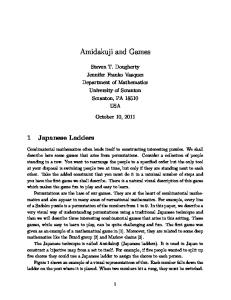
In the following example we visualize the algorithm, showing the process of adjusting and fixing the payoffs of the players. Example 4.1 Consider the neighbor game (P, v) where P = {1, . . . , 9} is the set of players. Let v be the characteristic function determined by the values of the neighbors as given in Table 2. One readily verifies that there is a unique optimal matching, viz., the matching S {1, 2} {2, 3} {3, 4} v(S) 3 10 10

{4, 5} 3

{5, 6} 3

{6, 7} 4

{7, 8} 6

{8, 9} 4

Table 2: The values of the neighbors in the neighbor game (P, v) µ = {(1, 2), (3, 4), (5, 6), (7, 8)}. As initial allocation we take x = (0, 3, 7, 3, 0, 3, 1, 5, 0). The game (P, v) and the allocation x are depicted in Figure 1. We put the players along the horizontal axis and their respective payoffs along the vertical axis. We connect the payoffs of the players so that the allocation x corresponds to a piecewise linear graph. Moreover, using Lemma 2.3 we immediately see that x is a core allocation: (i) The line through the payoffs of two matched neighbors runs exactly through the filled circle, which denotes half of the value of these neighbors; (ii) The line through the payoffs of two unmatched neighbors lies above or runs through the open circle, which denotes half of the value of these neighbors; (iii) All matched players receive a non-negative payoff; (iv) The unmatched player receives a payoff equal to zero. We apply the algorithm to x to find the leximax solution for the game (P, v). Note that P + = {1, . . . , 8} and P − = {9}. Set F := ∅.

payoff 8

6

4

2

3 1

10 2

10 3

3 4

3 5

6

4 6

7

4 8

9

player Figure 1: The initial allocation x 14

Loop I: (F 6= P + ) Step 1: S 1 = {3}. Step 2: C 1 = {3}, since player 3 is not adjustable (Definition 3.7 (1) with j = 1). As a consequence, F = {1, 2, 3, 4}. Since S 1 ⊆ F we go to Loop II. Loop II: (F = {1, 2, 3, 4} 6= P + ) Step 1: S 1 = {8}. Step 2: C 1 = ∅. Hence, S 2 = {8}. Step 3: I(8, x) = [7, 8] and by condition (B3)(a) with k + 1 = 9 we have ² = 1. The new allocation x is depicted in Figure 2.

payoff 8

6

4

2

3 1

10 2

10 3

3 4

3 5

6

4 6

7

4 8

9

player Figure 2: The allocation x that results from Loop II Loop III: (F = {1, 2, 3, 4} 6= P + ) Step 1: S 1 = {8}. Step 2: C 1 = {8}, since player 8 is not adjustable (Definition 3.7 (3)(a) with k + 1 = 9). As a consequence, F = {1, 2, 3, 4, 7, 8}. Since S 1 ⊆ F we go to Loop IV. Loop IV: (F = {1, 2, 3, 4, 7, 8} 6= P + ) Step 1: S 1 = {6}. Step 2: C 1 = ∅. Hence, S 2 = {6}. Step 3: I(6, x) = [5, 6] and by condition (B3)(a) with k + 1 = 7 and condition (B4) with j = 7 we have ² = 1. The new allocation x is depicted in Figure 3. Loop V: (F = {1, 2, 3, 4, 7, 8} 6= P + ) Step 1: S 1 = {6}. Step 2: C 1 = {6}, since player 6 is not adjustable (Definition 3.7 (3)(a) with k + 1 = 9). As a consequence, F = {1, 2, 3, 4, 5, 6, 7, 8}. Since S 1 ⊆ F we go to Loop VI. Loop VI: F = {1, 2, 3, 4, 5, 6, 7, 8} = P + Hence, we stop and Lmax(P, v) = x = (0, 3, 7, 3, 1, 2, 2, 4, 0). 15

¦

payoff 8

6

4

2

3 1

10 2

10 3

3 4

3 5

6

4 6

7

4 8

9

player Figure 3: The allocation x that results from Loop IV In the next lemma we prove that the recursive step is well-defined and that the algorithm does indeed yield the leximax solution. The lemma will also be used to prove that the algorithm terminates in a finite number of steps. Lemma 4.2 In the recursive step of the algorithm: (a) The players that we fix in the F -procedure are inadjustable and remain inadjustable if we do not change the payoffs of the players in F . (b) We only fix players in P + . Moreover, if we fix a player, then we fix his partner too. (c) If C 1 6= ∅, then let x∗ := xi where i ∈ C 1 . It holds that xi ≤ x∗ for all players i 6∈ F . (d) In the F -procedure we fix all players in C 1 . Hence, C 1 ∩ S 2 = ∅. (e) For ² > 0 sufficiently small, every player in S 2 satisfies the conditions (B1), (B2), (B3), and (B4). (f ) If i ∈ S 2 and j ∈ I(i, x), then j 6∈ F . (g) If i1 , i2 ∈ S 2 and i1 6= i2 , then not both i1 ∈ I(i2 , x) and i2 ∈ I(i1 , x). (h) The allocation y is well-defined and the payoffs of the fixed players do not change. Moreover, y is a core allocation and maxj6∈F yj < maxj6∈F xj . Proof. The proof is by induction on the number of loops. We assume that (a)-(h) hold for loops 1, . . . , t − 1 of the algorithm and that F 6= P + . Then, we prove that (a)-(h) hold for the t-th loop. The proof of (a)-(h) for the first loop of the algorithm has been omitted, since it is similar to the proof for the t-th loop. (a) By the induction hypothesis we only have to show that every unfixed player that we fix in the F -procedure is inadjustable by giving a condition in Definition 3.7 that is not satisfied. We distinguish among the three cases in Step 2. Let i ∈ C 1 . We may assume, without loss of generality, that I(i, x) = [i − 1, k]. Step a. Clearly, m ≥ i. Let j ∈ [i − 1, m], j 6∈ F . 16

Suppose |i − j| is even. Then, j ≥ i and I(j, x) = [j − 1, k]. Hence, j is not adjustable by Definition 3.7 (1) and m ∈ I(j, x). Suppose |i − j| is odd. Note that xj ≤ xi (otherwise i 6∈ S 1 ) and I(j, x) = [l, j + 1] for some l ≤ i − 1. Hence, j is not adjustable by Definition 3.7 (2), and i ∈ I(j, x). Step b. Clearly, m∗ ≥ i − 1. Let j ∈ [i − 1, m∗ + 1], j 6∈ F . We have xj ≤ xi (otherwise i 6∈ S 1 ). Suppose |i − j| is even. Note that xj ≤ xi ≤ xm∗ and I(j, x) = [j − 1, k]. Hence, j is not adjustable by Definition 3.7 (2) and m∗ ∈ I(j, x). Suppose |i − j| is odd. Note that I(j, x) = [l, j + 1] for some l ≤ i − 1. Hence, j is not adjustable by Definition 3.7 (2) and i ∈ I(j, x). Step c. Let j ∈ [i − 1, k], j 6∈ F . Suppose |i − j| is even. Then, j is not adjustable by Definition 3.7 (3). Suppose |i − j| is odd. Note that xj ≤ xi (otherwise i 6∈ S 1 ) and I(j, x) = [l, j + 1] for some l ≤ i − 1. Hence, j is not adjustable by Definition 3.7 (2) and i ∈ I(j, x). As one can verify easily, the discussed unsatisfied conditions above remain unsatisfied in the remainder of the algorithm if we do not change the payoffs of the players in F . Hence, the players that we fix in the F -procedure remain inadjustable in the remainder of the algorithm if we do not change the payoffs of the players in F . (b) Follows immediately from the F -procedure. (c) Suppose C 1 6= ∅. By definition of S 1 , it holds that the payoff of every player in C 1 is the same. So, we can define x∗ := xi for i ∈ C 1 . By definition of S 1 , we have that xi ≤ x∗ for all players i 6∈ F . (d) Let i ∈ C 1 . At least one of the conditions for i in Steps a, b, and c in the F procedure is satisfied. In any case, we fix player i. So, i 6∈ S 2 . Hence, C 1 ∩ S 2 = ∅. (e) From the definition of C 1 and (d), it follows that each player in S 2 is adjustable. This implies that for ² > 0 sufficiently small, every player in S 2 satisfies the conditions (B1), (B2), (B3), and (B4). (f ) The statement is clear for j = i. So, suppose j 6= i. Suppose j ∈ F . By (c), (h), and the induction hypothesis, there exists some player i0 ∈ F with xi0 ≥ xi , j ∈ I(i0 , x), and for which all players between i0 and j are fixed. By (b) and the induction hypothesis, the partner of j in µ is also fixed. One verifies that together with j ∈ I(i, x) this implies that i0 ∈ I(i, x). If |i − i0 | is odd, then i is not adjustable by Definition 3.7 (2). If |i − i0 | is even, then i is not adjustable for the same reason that i0 is not adjustable. So, in either case i is not adjustable, contradicting (b). Hence, our assumption that j ∈ F is false. (g) Let i1 , i2 ∈ S 2 and i1 6= i2 . Suppose that both i1 ∈ I(i2 , x) and i2 ∈ I(i1 , x). Then, 17

|i1 − i2 | is odd. Since i1 , i2 ∈ S 2 ⊆ S 1 , we have xi1 = xi2 . So, i1 and i2 are not adjustable by Definition 3.7 (2). This contradicts i1 , i2 ∈ S 2 . (h) It follows from (g) that y is well-defined. It follows from (f ) that the payoffs of fixed players do not change. The inequality maxj6∈F yj < maxj6∈F xj follows from the definition of S 1 and the definition of the allocation y. One easily verifies that y ∈ Core(P, v) by checking the conditions in Lemma 2.3. We have omitted this part of the proof since it runs similarly to the proof of y ∈ Core(P, v) in the ‘only if’-part of the proof of Theorem 3.9. 2 The following lemma shows that the algorithm terminates after a finite number of steps. Lemma 4.3 After at most 2p + 1 loops the number of fixed players increases strictly. Proof. Consider a loop of the algorithm for which F 6= P + in Step 1. Let x be the allocation in Step 1. Suppose that the number of fixed players does not increase strictly. In other words, suppose that we do not fix any player in the F -procedure. Then we go to Step 3 with S 2 = S 1 6= ∅. We make the following three observations. Observation 1. If there is an equality in (B1) or (B2) for a player i ∈ S 2 , then i will be an inadjustable player in the next loop. Since i remains a player with highest payoff among the non-fixed players, he will be fixed in the next loop. Observation 2. If there is an equality in (B3) for a player i ∈ S 2 , then: either or

1) 2)

i is fixed in the next loop (for sure if k + 1 ∈ F or k + 1 ∈ P − ) the maximal relevant interval of i becomes strictly larger in the next loop (only possible if k + 1 ∈ P + \F ),

where I(i, x) is, without loss of generality, assumed to be of the form [i − 1, k]. By Lemma 4.2 (g), there can be at most p subsequent loops in which 1) we do not fix any player in S 2 and 2) in which the maximal relevant interval of a player in S 2 becomes strictly larger. Observation 3. There can be at most p subsequent loops in which we do not fix any player and in which there is no equality in (B1), (B2), or (B3). This follows since a player j appears at most once in an equality in (B4). From the three observations one can conclude that after at most 1 + p + p subsequent loops we fix a player. This proves the lemma. 2

Lemma 4.4 The algorithm for finding the leximax solution of a neighbor game takes O(p3 ) time. 18

Proof. It takes at most O(p2 ) time to calculate a core allocation, which serves as initial allocation for the algorithm (see footnote on the initial allocation in the algorithm). It follows from Lemma 4.3 that the algorithm terminates after at most p(2p+1) loops. Since each loop takes at most O(p) time we conclude that the algorithm is of order p3 . 2

19

References Arin J, I˜ narra E (1997) Consistency and Egalitarianism: The Egalitarian Set. SEEDS Discussion Paper 163, University of the Basque Country, Bilbao, Spain Arin J, Kuipers J, Vermeulen D (1998) An Axiomatic Approach to Egalitarianism in TU-games. IEP Discussion Paper 98-05, Instituto de Econom´ıa P´ ublica, University of the Basque Country, Bilbao, Spain Curiel I, Potters J, Rajendra Prasad V, Tijs S, Veltman B (1994) Sequencing and Cooperation. Operations Research 42: 566-568 Hamers H, Klijn F, Solymosi T, Tijs S, Vermeulen D (2003) On the Nucleolus of Neighbor Games. European Journal of Operational Research 146: 1-18 Hamers H, Klijn F, Solymosi T, Tijs S, Villar JP (2002) Assignment Games satisfy the CoMa-property. Games and Economic Behavior 38: 231-239 Moulin H (1988) Axioms of Cooperative Decision Making. Cambridge University Press, Cambridge Owen G (1986) Values of Graph-Restricted Games. SIAM Journal of Algebraic and Discrete Methods 7: 210-220 Potters J, Reijnierse H (1995) Γ-Component Additive Games. International Journal of Game Theory 24: 49-56 Schmeidler D (1969) The Nucleolus of a Characteristic Function Game. SIAM Journal on Applied Mathematics 17: 1163-1170 Shapley L, Shubik M (1972) The Assignment Game I: The Core. International Journal of Game Theory 1: 111-130 Sharkey W (1982) Cooperative Games with Large Cores. International Journal of Game Theory 11: 175-182

20