New Results on the Capacity of the Gaussian Cognitive Interference Channel Stefano Rini, Daniela Tuninetti, and Natasha Devroye Department of Electrical and Computer Engineering University of Illinois at Chicago Email: {srini2, danielat, devroye}@uic.edu
Abstract—The capacity of the two-user Gaussian cognitive interference channel, a variation of the classical interference channel where one of the transmitters has knowledge of both messages, is known in several parameter regimes but remains unknown in general. In this paper, we consider the following achievable scheme: the cognitive transmitter pre-codes its message against the interference created at its intended receiver by the primary user, and the cognitive receiver only decodes its intended message, similar to the optimal scheme for “weak interference”; the primary decoder decodes both messages, similar to the optimal scheme for “very strong interference”. Although the cognitive message is pre-coded against the primary message, by decoding it, the primary receiver obtains information about its own message, thereby improving its rate. We show: (1) that this proposed scheme achieves capacity in what we term the “primary decodes cognitive” regime, i.e., a subset of the “strong interference” regime that is not included in the “very strong interference” regime for which capacity was known; (2) that this scheme is within one bit/s/Hz, or a factor two, of capacity for a much larger set of parameters, thus improving the best known constant gap result; (3) we provide insights into the trade-off between interference pre-coding at the cognitive encoder and interference decoding at the primary receiver based on the analysis of the approximate capacity results.
I. I NTRODUCTION The cognitive interference channel [1] is a well studied channel model inspired by the newfound abilities of cognitive radio technology and its potential impact on spectral efficiency in wireless networks [2]. This channel model consists of a two-user interference channel, where one transmitter-receiver pair is referred to as the primary user and the other as the cognitive user. As opposed to the classical interference channel, the cognitive transmitter has full non-causal knowledge of both messages, idealizing the cognitive user’s ability to detect transmissions taking place in the network.1 The primary transmitter has knowledge of its own message only. Past work. The cognitive interference channel was first posed in an information theoretic framework in [1], where an achievable rate region (for discrete memoryless channels) and a broadcast-channel-based outer bound (for Gaussian channels only) were proposed. The first capacity results were 1 This channel has also been termed the interference channel with unidirectional cooperation [3] or the interference channel with degraded message set [4].
determined in [5], [4] for channels with “weak interference” at the primary receiver. In this regime, the cognitive transmitter pre-codes its message against the interference created at its receiver by the primary message, while the primary receiver treats the interference from the cognitive transmitter as noise. In contrast, in the regime of “very strong interference” at the primary receiver, capacity is achieved by simple superposition coding at the cognitive transmitter and by having both receivers decode both messages [6]. For the general cognitive interference channel, the largest known achievable rate region is found in [7] (where the inclusion of all previously proposed inner bounds is formally shown), while the tightest known outer bound is in [3] (based on a broadcast-channel-based technique from [8]). While in general the capacity region remains unknown, in Gaussian noise, we recently demonstrated an achievable rate region which lies to within 1.87 bits/s/Hz from capacity [9]. Contributions. In this paper, we: 1) Derive a new capacity result by showing the achievability of an outer bound originally presented in [3] for a subset of the “strong interference” regime. 2) Prove capacity to within one bit/s/Hz or to within a factor two in a large parameter region. 3) Highlight how non-perfect (partial) interference “precancellation” at the cognitive user boosts the rate of the primary user and give numerical examples to quantify the rate improvements. Organization. The rest of the paper is organized as follows: Section II formally defines the channel model and summarizes known results for the Gaussian channel; Section III proves the new capacity result; Section IV analyzes the capacity achieving scheme with perfect “pre-cancellation” of the interference and shows two new approximate capacity results; Section V focuses on the achievable rates with partial interference “precancellation”; and Section VI concludes the paper. II. C HANNEL
MODEL AND KNOWN RESULTS
A two-user InterFerence Channel (IFC) is a multi-terminal network with two senders and two receivers. The inputs (X1 , X2 ) are related to the outputs (Y1 , Y2 ) by a memoryless channel with transition probability PY1 ,Y2 |X1 ,X2 . Each
Theorem II.1. Outer bound of [9]. The capacity region of the G-CIFC is included in: R1 ≤ C (αP1 ) , � � p R2 ≤ C |b|2 P1 + P2 + 2 α ¯ |b|2 P1 P2 , � � p R1 + R2 ≤ C |b|2 P1 + P2 + 2 α ¯ |b|2 P1 P2 � � 1 + max{1, |b|2 }αP1 , + log 1 + α|b|2 P1 Fig. 1.
The G-CIFC.
transmitter i, i ∈ {1, 2}, wishes to communicate a message Wi to receiver i. Each message Wi , i ∈ {1, 2}, is uniformly distributed on {1, . . . , 2N Ri }, where N represents the blocklength and Ri the transmission rate. The two messages are independent. In the classical IFC, the two transmitters operate independently. Here we consider a variation of this set up by assuming that transmitter 1 (referred to as the cognitive user), in addition to its own message also knows the message of transmitter 2 (referred to as the primary user). A rate pair (R1 , R2 ) is achievable for a CIFC if there exists a sequence of encoding functions
(1a) (1b)
(1c)
taken over the union of all α ∈ [0, 1]. Theorem II.2. “Weak interference” capacity of [4, Lemma 3.6] and [5, Th. 4.1]. If |b| ≤ 1,
(“weak interference” regime/condition)
(2)
the outer bound of Th.II.1 is tight. Theorem II.3. “Very strong interference” capacity of [12, Thm. 6] extended to complex-valued channels. When p (|a|2 − 1)P2 − (|b|2 − 1)P1 − 2 a − |b| P1 P2 ≥ 0,
and |b| > 1 (“very strong interference” regime/condition) (3) the outer bound of Th.II.1 is tight.
X1N = X1N (W1 , W2 ),
X2N = X2N (W2 ),
and a sequence of decoding functions
such that
c1 = W c1 (Y N ), W 1
c2 = W c2 (Y N ), W 2
h i ci = max P W 6 Wi → 0,
i∈{1,2}
as N → ∞.
The capacity region is the convex closure of the set of achievable rates [10]. A complex-valued Gaussian CIFC (G-CIFC) in standard form, as represented in Fig. 1, has outputs: Y1 = X1 + aX2 + Z1 , Y2 = |b|X1 + X2 + Z2 , for a, b ∈ C, where the inputs are subject to the power constraint E[|Xi |2 ] ≤ Pi , i ∈ {1, 2}, and where the additive proper-complex Gaussian noises Z1 and Z2 have zero mean and unit variance. Without loss of generality [11], the phase of b can be taken to be zero. When a = |b|−1 , one channel output is a degraded version of the other output. In particular, when |b| ≤ 1, Y2 is a degraded version of Y1 , and when |b| > 1, Y1 is a degraded version of Y2 . We refer to this particular channel as the degraded G-CIFC. The capacity region of the G-IFC is not known in general. We next summarize known capacity results for the G-CIFC. We define C(x) := log(1 + x).
Proof: For complex-valued G-CIFC with |b| > 1, the outer bound of Th.II.1 is achievable by the superposition-only scheme of [12] if I(Y1 ; X1 , X2 ) ≥ I(Y2 ; X1 , X2 ) for all input distributions, that is, if E[|Y1 |2 ] − E[|Y2 |2 ] = (|a|2 − 1)P2 − (|b|2 − 1)P1 + p + 2 P1 P2 (Re{a∗ ρ} − |b|Re{ρ}) ≥ 0, ∀|ρ| ≤ 1.
(4)
Let ρ = |ρ|ejφρ and a = |a|ejφa . We have
Re{a∗ ρ} − |b|Re{ρ} = |ρ||a| cos(φρ − φa ) − |ρ||b| cos(φρ ) = a − |b| · |ρ| cos(φ),
for some angle φ. The condition in (4) is thus verified for all |ρ| cos(φ) ∈ [−1, +1] if it is verified for |ρ| cos(φ) = −1. Theorem II.4. Constant gap of [9]. The gap between the outer bound in Th.II.1 and the achievable scheme of [9] is at most 1.87 bits/s/Hz. Fig. 2 shows the region where capacity is known (shaded region) and where only constant gap results are available (white region) in the (a, |b|)-plane for a ∈ R and P1 = P2 . III. N EW CAPACITY
RESULTS
We now show the achievability of the outer bound of Th.II.1 for a subset of |b| > 1 not included in the “very strong interference” regime of Th.II.3. We first present an achievable scheme and then derive the conditions under which it is capacity achieving.
Fig. 2. A representation of the known capacity results for the real-valued GCIFC with P1 = P2 and (a, |b|) ∈ [−5, 5] × [0, 5]. The “weak interference” regime has solid light blue fill, while the “very strong interference” regime has dotted green lines.
A. Achievable scheme Consider the achievable scheme of [13] where only R1c and R2pa are non zero2 , that is: N • the primary message W2 is encoded in X2 , N • the cognitive message W1 is encoded in U1c , N • U1c is Dirty Paper Coded (DPCed) against the interference created by X2N at the cognitive receiver, N N N • X1 is a function of X2 and U1c , N • the cognitive receiver decodes U1c , and, N N • the primary receiver jointly decodes U1c and X2 . This scheme achieves the following region: R1 R2 R1 + R2
≤
I(Y1 ; U1c ) − I(U1c ; X2 ),
(5a)
≤
I(Y2 ; U1c , X2 ),
(5c)
≤
I(Y2 , U1c ; X2 ) = I(Y2 ; U1c , X2 ) + � � − I(Y2 ; U1c ) − I(U1c ; X2 ) , (5b)
for any distribution pU1c X1 X2 . For the G-CIFC, we restrict our attention to the case: X1c
∼
X2
∼
X1
=
U1c
=
Y1
=
Y2
=
NC (0, αP1 ), α ∈ [0, 1],
NC (0, P2 ) , X1c ⊥ X2 , r α ¯ P1 X1c + X2 , P2 X1c + λX2 , λ ∈ C, ! r α ¯ P1 X1c + a + X2 + Z1 , P2 s 2P α ¯ |b| 1 |b|X1c + 1 + X2 + Z2 . P2
(6a) (6b) (6c) (6d) (6e)
(6f)
The parameter α denotes the fraction of power that encoder 1 employs to transmit its own message versus the power to broadcast X2 . For α = 0, transmitter 1 uses all its power to broadcast X2 as in a virtual Multiple Input Single Output (MISO) channel. When α = 1, transmitter 1 utilizes all its 2 This scheme can also be obtained as a special case of the region of [3, Th. 1] and [14].
power to transmit X1c . With the choices in (6), the region in (5) becomes: ! r α ¯ P1 R1 ≤ f a + , 1; λ , (7a) P2 p R2 ≤ C(P2 + |b|2 P1 + 2 α ¯ |b|2 P1 P2 ) + ! r 1 αP ¯ 1 1 −f + , ;λ , (7b) |b| P2 |b|2 p R1 + R2 ≤ C(P2 + |b|2 P1 + 2 α ¯ |b|2 P1 P2 ), (7c)
for
f (h, σ 2 ; λ) , I(X1c + hX2 + σZ1 ; U1c ) − I(U1c ; X2 ) = log
where
σ 2 + αP1 2 , 2 λ 1 |h| P2 σ 2 + αP1αP +|h|2 P2 +σ2 λCosta (h,σ2 ) − 1 λCosta (h, σ 2 ) ,
αP1 h. αP1 + σ 2
The parameter λ controls how much of the interference created by X2 is “pre-canceled” and � � f (h, σ 2 ; λ) ≤ f h, σ 2 ; λCosta (h, σ 2 ) = C αP1 /σ 2 ,
i.e., λ = λCosta (h, σ 2 ) achieves the “interference free” rate as shown by Costa in [15]. B. The pre-coding parameter λ
As mentioned before, the parameter λ controls the amount of interference “pre-cancellation” achievable with DPC at transmitter 1. With λ = 0, no DPC is performed at transmitter 1 and the interference due to X2 is treated as noise. On the other hand, with ! r α ¯ P1 λ = λCosta a + , 1 , λCosta 1 , P2 the interference due to X2 at receiver 1 is completely “precanceled”, thus achieving the maximum possible rate R1 . Different values of λ are not usually investigated because, as long as the interference is a nuisance (i.e., no node in the network has information to extract from the interference), the best is to completely “pre-cancel” it by using λ = λCosta (h, σ 2 ). However, λ influences not only the rate R1 in (7a), but also the rate R2 in (7b). An interesting question is whether λ 6= λCosta 1 , although it does not achieve the largest possible R1 , would improve the achievable region by sufficiently boosting the rate R2 . We comment on this question later on. At this point we make the following observation: R1 is a concave function in λ, symmetric around λ = λCosta 1 and with a global maximum at λ = λCosta 1 , while R2 is a convex function in λ, symmetric around λ = λCosta 2 and with a global minimum at λ = λCosta 2 , where ! r 1 α ¯ P1 1 λCosta + , , λCosta 2 . |b| P2 |b|2
Fig. 4. A representation of the capacity result of Th.III.1 for a real-valued G-CIFC with P1 = P2 = 10 and (a, |b|) ∈ [−5, 5] × [0, 5]. The “weak interference” regime has solid light blue fill, the “very strong interference” regime has dotted green lines, while the “primary decodes cognitive” region has dotted navy blue lines.
Fig. 3. The bound for R1 in (7a) (bottom) and the√bound for R√ 2 in (7b) (top) as a function of λ ∈ R, for P1 = P2 = 6, b = 2 and a = 0.3 and α = 0.5.
Fig. 3 shows R1 in (7a)√and R2 in √ (7b) as a function of λ ∈ R, for P1 = P2 = 6, b = 2, a = 0.3 and α = 0.5. C. New “strong interference” capacity result We now determine the conditions under which the outer bound of Th.II.1 can be achieved by the region in (7). Theorem III.1. The “primary decodes cognitive” regime. When |b| > 1 and 2 P2 |1 − a|b||2 ≥ (|b|2 − 1)(1 + P1 + |a|2 P2 ) − P1 P2 1 − a|b| , (8a) p P2 |1 − a|b||2 ≥ (|b|2 − 1)(1 + P1 + |a|2 P2 + 2Re{a} P1 P2 ), (8b)
the outer bound of Th.II.1 is tight.
The “primary decodes cognitive” regime, illustrated in Fig. 4 in the (a, |b|)-plane for a ∈ R and P1 = P2 = 10, covers parts of the “strong interference” regime where capacity was known to within 1.87 bits/s/Hz only. It also shows that the scheme in (7) is capacity achieving for part of the “very strong interference” region, thus providing an alternative capacity achieving scheme to superposition coding [12]. Proof: The achievable scheme in (7) for |b| > 1 and λ = λCosta 1 achieves (1a)=(7a) and (1c)=(7c) (and (1b) is redundant). Therefore the outer bound of Th.II.1 is achievable when ((7a)+(7b))≥(1b), that is when r � � α ¯ P1 C(αP1 ) = f a + , 1; λCosta 1 P2 r �1 � α ¯ P1 1 ≥f + , 2 ; λCosta 1 , ∀α ∈ [0, 1]. (9) |b| P2 |b| After some algebra, the inequality (9) can be shown to be equivalent to � 2 Q(α) , P2 1 − a|b| (αP1 + 1) − (|b|2 − 1) P1 + |a|2 P2 + � p + 2Re{a} α ¯ P1 P2 + 1 ≥ 0, ∀α ∈ (0, 1]. (10)
The inequality in (10) is verified if Q(0) ≥ 0 (which corresponds to the condition in (8b)) and Q(1) ≥ 0 (which corresponds to the condition in (8a)). Previous capacity results for the G-CIFC imposed conditions on the channel parameters that lent themselves well to “natural” interpretations. For example, the “weak interference” condition I(Y1 ; X1 |X2 ) ≥ I(Y2 ; X1 |X2 ) suggests that decoding X1 at receiver 2, even after having decoded the intended message in X2 , would constrain the rate R1 too much, thus preventing it from achieving the interference-free rate in (1a). The “very strong interference” condition I(Y1 ; X1 , X2 ) ≥ I(Y2 ; X1 , X2 ) suggests that requiring receiver 1 to decode both messages should not prevent achieving the maximum sum-rate at receiver 2 given by (1c). A similar intuition about the new “primary decodes cognitive” capacity condition in (8) does not emerge from the proof of Th.III.1. For this reason we devote the next sections to analyze the achievable scheme of Section III-A in more detail. We shall consider the case of perfect interference “pre-cancellation” at receiver 1 (i.e., λ = λCosta 1 ) and partial (or non-perfect) interference “precancellation” at receiver 1 (i.e., λ 6= λCosta 1 ) separately. IV. P ERFECT
INTERFERENCE “ PRE - CANCELLATION ”
We next establish approximate capacity results by comparing the achievable performance of the scheme in Section III-A with perfect interference “pre-cancellation” at the cognitive receiver (i.e., λ = λCosta 1 ) to the outer bound in Th.II.1. In particular, we show a parameter range where capacity can be achieved within one bit/s/Hz, or within a factor two. A. Approximate capacity results Assume λ = λCosta 1 . For α = 0, the achievable scheme in (7) is optimal and achieves the MISO point A in Fig. 5. Moreover, when the conditions in (8) are verified, the outer bound of Th.II.1 is achievable for all α ∈ [0, 1]. In general, however the inner and outer bounds meet for some α ∈ [0, 1]. In particular, from the proof of Th.III.1, it is possible to achieve the outer bound point for α = 1 whenever the condition in (8a) holds. We use this observation to reduce
Fig. 6. The region where the condition in (12) is verified, for different values of P1 = P2 = P . Fig. 5. A representation of the proof of Th.IV.1: the solid blue line is the outer bound in (1) and the dotted blue line the outer bound in (11); the green hatched region is the achievable region obtained with time sharing between the points A and C, while the green dotted line is the region in the converse of the multiplicative gap.
the additive gap of Th. II.4. In addition we also provide a multiplicative gap. The additive bound is effective at high SNR, where the difference between inner and outer bound is small in comparison to the magnitude of the capacity region, while the multiplicative bound is useful at low SNR, where the ratio between inner and outer bound is a more indicative measure of their distance. Theorem IV.1. When the condition in (8a) holds the outer bound of Th.II.1 is achievable to within one bit/s/Hz or to within a factor two. Proof: By choosing the two values of α that maximize each bound in (1), we obtain that the outer bound of Th.II.1 for |b| > 1 is contained in R1 R1 + R2
≤
≤
C(P1 ), p p C(( |b|2 P1 + P2 )2 ),
(11a) (11b)
whose Pareto-optimal corner points (see Fig. 5) are the MISO point � � p p A = 0, C(( |b|2 P1 + P2 )2 and the point � � p p B = C(P1 ), C(( |b|2 P1 + P2 )2 ) − C(P1 ) .
When condition (8a) is verified, it is possible to achieve the point of the outer bound of Th.II.1 corresponding to α = 1 given by (see Fig. 5) � C = C(P1 ), C(|b|2 P1 + P2 ) − C(P1 ) .
Since points B and C have the same R1 -coordinate, a constant additive gap is readily shown by proving that the difference of the R2 -coordinates is bounded. We have: ! p 2 |b|2 P1 P2 (B) (C) R2 − R2 = C 1 + |b|2 P1 + P2 ! r P2 ≤C ≤ C(1) = log(2) = 1 bit, 1 + P2
where the largest gap is for |b|2 P1 = P2 + 1. For the multiplicative gap, it is sufficient to show that (C) (C) (B) (B) 2(R1 + R2 ) ≥ R1 + R2 (see Fig. 5), that is p (1 + |b|2 P1 + P2 )2 ≥ 1 + |b|2 P1 + P2 + 2 |b|2 P1 P2 ⇐⇒ p p | |b|2 P1 − P2 |2 + (|b|2 P1 + P2 )2 ≥ 0,
which is always verified. In Fig. 6 we plot the region where the condition in (8a) holds for a ∈ R and for increasing values of P1 = P2 = P , that is, the region of (a, |b|) pairs that satisfy P (P + 1)|1 − a|b||2 ≥ (|b|2 − 1)(P + 1 + |a|2 P ).
(12)
We notice that when a|b| = 1 (degraded channel), the condition in (12) is satisfied by a = |b| = 1 only. As we increase P , the set of (a, |b|) pairs for which (12) is satisfied enlarges and converges to a|b| = 6 1. In other words, for high-SNR, the scheme in Section III-A with λ = λCosta 1 is within one bit/s/Hz or a factor two of capacity for all channel parameters, except for the degraded channel. However, for finite SNR, there exists a region around the degraded line a|b| = 1 for which the approximate capacity result of Th. IV.1 does not hold. This is so because in this regime λCosta 1 ≈ λ Costa 2 and thus the choice λ = λCosta 1 gives a value for (7b) very close to its minimum (see Fig. 3) and prevents the achievability of the point C. This observation motivates the study of imperfect, or partial, interference “pre-cancellation” (λ 6= λCosta 1 ) at the cognitive receiver. V. PARTIAL
INTERFERENCE
“ PRE - CANCELLATION ”
A. On the utility of partial interference “pre-cancellation” In order to understand the rate improvements from partial interference “pre-cancellation” in the achievable scheme of Section III-A, we first revisit the gap result of Th.II.4 from [9]. In [9, Sec. IV.B] we showed that in the subset of the “strong interference” regime where Th. IV.1 does not hold, choosing λ = λCosta 1 + ǫ, with ǫ an appropriate decreasing function of the transmit powers, yields a gap to capacity of at most 1.87 bits/s/Hz. This choice of λ can be interpreted as follows. From (5b), we see that U1c plays the role of side information at receiver 2 when decoding X2 . The DPC coefficient λ = λCosta 1 + ǫ favors the decoding of U1c at receiver 2 while slightly degrading the rate of user 1 in (5a). In particular,
the achievable scheme in Section III-A for λ = λCosta achieves:
1
+ǫ
R1 ≤ (7a) = log (1 + αP1 ) + � � (αP1 + 1)2 P2 2 √ − log 1 + |ǫ| , αP1 (1 + P1 + |a|2 P2 + 2Re{a} α ¯ P1 P2 ) � � p R2 ≤ (7b) = log 1 + |b|2 P1 + P2 + 2 α ¯ |b|2 P1 P2 + � 1 + log + 1 + α|b|2 P1 ! (α|b|2 P1 + 1)P2 2 p + |ǫ + ∆λ | , αP1 (1 + |b|2 P1 + P2 + 2 α ¯ |b|2 P1 P2 ))
where ∆λ = λCosta 1 − λCosta 2 . Let ǫ be small and with the same phase as ∆λ . From the above expressions, we see that the decrease of R1 is of the order O(|ǫ|2 ), while the increase of R2 is of the order O(|ǫ|). This demonstrates how one can trade residual interference at the cognitive receiver for rate improvement at the primary receiver, which makes use of U1c to decode its own message. B. On the limits of partial interference “pre-cancellation” A natural question at this point is whether it is possible to achieve capacity by using the strategy in Section III-A with λ = λCosta 1 + ǫ. Unfortunately, the answer is negative:
Lemma V.1. The achievability of the outer bound of Th.II.1 using the achievable scheme of Section III-A can be shown only in the “primary decodes cognitive” regime of Th.III.1. Proof: This result is shown by observing that only one choice of α and λ in (7) achieves both the sum rate bound in (1c) and the R1 bound in (1a)–the choice which corresponds to the “primary decodes cognitive” regime of Th.III.1. To distinguish the parameters α in the inner and outer bound, let α(out) be the α parameter in the outer bound in (1) and α(in) be the α parameter in (7). Consider the region (1) for a fixed α(out) . We first notice that to achieve the sum rate outer bound in (1c) we have to pick the α(in) in (7) such that α(in) ≤ α(out) (because the expressions are monotonically decreasing in α). On the other hand, the maximum rate R1 in (7a) for α(in) ≤ α(out) is always smaller than the outer bound for R1 in (1a), with equality only if α(in) = α(out) and λ = λCosta 1 . So to achieve both the sum rate outer bound and the R1 rate outer bound we must have α(in) = α(out) and λ = λCosta 1 , which are the specific assignments considered in Theorem III.1. C. Further considerations on the utility of partial interference “pre-cancellation” In spite of the result of Lemma V.1, we next show that the largest inner bound region with the scheme of Section III-A is achieved by λ 6= λCosta 1 . Finding the λ that minimizes the distance between the inner and outer bounds is analytically too involved. For this reason we consider the simpler problem of determining the value of λ that maximizes the sum rate.
Lemma V.2. When |b| > 1 and the “very strong interference” condition is not satisfied, setting λ to a solutions of H −1 − H1−1 )|λ|2 + − P2 (|b|2 H2−1 − H1−1 + 2 αP 1 �p � 2 α ¯ P1 P2 (|b|2 H2−1 − H1−1 ) + P2 (|b|H2−1 − Re{a}H1−1 ) Re{λ} αP1 (|b|2 H2−1 − H1−1 ) = 0.
for
(13)
p ¯ P1 P2 , H1 = E[|Y1 |2 ] = 1 + |a|2 P2 + P1 + 2Re{a} α p 2 2 H2 = E[|Y2 | ] = 1 + P2 + |b| P1 + 2 α ¯ |b|2 P1 P2 ,
yields the largest achievable sum rate in the scheme of Section III-A for a given α ∈ [0, 1]. Proof: This result is established by observing that (7c) is the maximum achievable sum rate for a fixed α. Then, the λ that maximizes the sum rate must satisfy (7a) + (7b) = (7c), that is, r r � �1 � � α ¯ P1 α ¯ P1 1 f a+ , 1; λ = f + , 2 ; λ . (14) P2 |b| P2 |b|
After some algebra, we rewrite the condition in (14) as in (13). Notice that there exist real-valued solutions (i.e., λ ∈ R) for in (13). Indeed, when the “very strong interference” condition is not verified, and |b| ≥ 1, we have H1 ≤ H2 for all α ∈ [0, 1], and thus it follows that: the coefficient of |λ|2 is negative, the coefficient of Re{λ} is positive, and the constant term is positive. By choosing Im{λ} = 0, the equation (13) reduces to the quadratic function in Re{λ}, which has positive definite determinant and thus has at least one real-valued solution. D. Numerical results For the numerical results in the following we restrict ourselves to real-valued input/output G-CIFC so as to reduce the dimensionality of the search space for the optimal parameter values. Although choosing λ according to Lemma V.2 does not guarantee achieving the largest inner bound, we next show by numerical evaluations that significant rate improvements can be obtained when compared to choosing λ = λCosta 1 . Fig. 7 shows the position of the point � � D(λ) = (7a), min{(7b), (7c) − (7a)} in the range λ ∈ [0, 2λCosta 1 ], for a fixed α(in) , together the outer bound point C for α(out) = α(in) . Under the “primary decodes cognitive” condition, D(λCosta 1 ) = C for every α ∈ [0, 1]. However, here we show a channel where the condition in (8a) is not satisfied. In this case the choice λ = λCosta 1 minimizes the distance of the R1 -coordinate between D and C, but it does not minimize the Euclidean distance between the two points. The choice of λ as in Lemma V.2 minimizes the distance between the sum rate inner and outer bounds. The following is another example to show that partial interference “pre-cancellation” (λ 6= λCosta 1 ) yields an
Fig. 7. A plot of the points C(λ) and D(λ) for α = 0.5, together with the “strong interference” bound for √ √ the real-valued G-CIFC with parameters P1 = P2 = 6, b = 2 and a = 0.3.
Fig. 8. A portion of the achievable region in (7) for λ = λCosta (labeled as “perfect DPC”), the optimal λ ∈ [0, 2λCosta ] (labeled as “any DPC”), and λ chosen as in Lemma V.2 (labeled as “sum rate optimal”) for the real-valued G-CIFC with parameters P1 = P2 = 6, b = 3 and a = 2.
achievable region larger than with perfect interference “precancellation” (λ = λCosta 1 ). Fig. 8 illustrates the achievable region obtained with the choice of λ as in Lemma V.2. For this choice of parameters, the region obtained by considering any λ ∈ [0, 2λCosta 1 ] coincides with the region obtained by choosing λ as in Lemma V.2. The achievable rate region for λ = λCosta 1 is also provided for reference. Although numerical evaluations show that this is not the case in general, it is interesting to note that this choice of λ has the same achievable rate region as the one obtained using any (optimal) values of λ. VI. C ONCLUSION
AND
F UTURE W ORK
In this paper we presented a new capacity result for the Gaussian cognitive interference channel in a subset of the
channel parameter space which we term the “primary decodes cognitive” regime. We derived an additive and a multiplicative approximate capacity result that provides important insight on the fundamental features of the capacity achieving scheme. In particular, we show how pre-coding against the interference for one user can be used to boost the rate of the other user. Numerical results further verify that significant rate improvements can be obtained. While this result extends the parameter regimes in which capacity for the Gaussian cognitive interference channel is known, it still remains unknown in general. The achievable region of [13] provides a comprehensive inner bound that can potentially yield new capacity results. Only some specific choices of parameters for this region have been considered so far and we thus expect that additional results may be derived from this region. On the other hand, tighter outer bounds for the capacity region are also probably necessary. When the Gaussian cognitive interference channel reduces to a broadcast channel, the outer bound is not tight, suggesting that the outer bound may be loose in an even larger region. R EFERENCES [1] N. Devroye, P. Mitran, and V. Tarokh, “Achievable rates in cognitive radio channels,” IEEE Trans. Inf. Theory, vol. 52, no. 5, pp. 1813–1827, May 2006. [2] A. Goldsmith, S. Jafar, I. Maric, and S. Srinivasa, “Breaking spectrum gridlock with cognitive radios: An information theoretic perspective,” Proc. IEEE, 2009. [3] I. Maric, A. J. Goldsmith, G. Kramer, and S. Shamai, “On the capacity of interference channels with one cooperating transmitter,” European Transactions on Telecommunications, vol. abs/0710.3375, 2008. [4] W. Wu, S. Vishwanath, and A. Arapostathis, “Capacity of a class of cognitive radio channels: Interference channels with degraded message sets,” Information Theory, IEEE Transactions on, vol. 53, no. 11, pp. 4391–4399, Nov. 2007. [5] A. Jovicic and P. Viswanath, “Cognitive radio: An information-theoretic perspective,” Information Theory, 2006 IEEE International Symposium on, pp. 2413–2417, July 2006. [6] I. Maric, R. Yates, and G. Kramer, “Capacity of interference channels with partial transmitter cooperation,” Information Theory, IEEE Transactions on, vol. 53, no. 10, pp. 3536–3548, Oct. 2007. [7] S. Rini, D. Tuninetti, and N. Devroye, “New inner and outer bounds for the discrete memoryless cognitive channel and some capacity results,” IEEE Transactions on Information Theory, 2010, submitted. [8] C. Nair and A. E. Gamal, “An outer bound to the capacity region of the broadcast channel,” Information Theory, IEEE Transactions on, vol. 53, no. 1, pp. 350–355, Jan. 2007. [9] S. Rini, D. Tuninetti, and N. Devroye, “The capacity region of gaussian cognitive radio channels to within 1.87 bits,” Proc. IEEE ITW Cairo, Egypt, Jan. 2010. [10] J. A. T. Thomas M. Cover, Elements of Information Theory. WileyInterscience, 1991. [11] S. Rini, “On the role of cognition and cooperation: an information theoretic prospective,” available at http://sites.google.com/site/rinistefano/ my-thesis-proposal, Nov. 2009, preliminary examination. [12] I. Maric, R. Yates, and G. Kramer, “The capacity region of the strong interference channel with common information,” Signals, Systems and Computers. Conference Record of the Thirty-Ninth Asilomar Conference on, pp. 1737–1741, Nov. 2005. [13] S. Rini, D. Tuninetti, and N. Devroye, “State of the cognitive interference channel: a new unified inner bound,” in International Zurich Seminar on Communications, March 2010, p. 57. [14] Y. Cao and B. Chen, “Interference channel with one cognitive transmitter,” in Asilomar Conference on Signals, Systems, and Computers, Nov. 2008. [15] M. Costa, “Writing on dirty paper (corresp.),” IEEE Transactions on Information Theory, vol. 29, no. 3, pp. 439–441, 1983.