PHYSICAL REVIEW B

VOLUME 53, NUMBER 15

15 APRIL 1996-I

Parametric conductance correlation for irregularly shaped quantum dots Henrik Bruus CNRS–CRTBT, 25 Avenue des Martyrs, BP166, F-38042 Grenoble Ce´dex 9, France

Caio H. Lewenkopf Instituto de Fı´sica, Universidade de Sa˜o Paulo, Caixa Postal 66318, 05389-970, Sa˜o Paulo, Brazil

Eduardo R. Mucciolo

NORDITA, Blegdamsvej 17, DK-2100 Copenhagen O ” , Denmark ~Received 20 October 1995! We propose the autocorrelator of conductance peak heights as a signature of the underlying chaotic dynamics in quantum dots in the Coulomb blockade regime. This correlation function is directly accessible to experiments and its decay width contains interesting information about the underlying electron dynamics. Analytical results are derived in the framework of random matrix theory in the regime of broken time-reversal symmetry. The final expression, upon rescaling, becomes independent of the details of the system. For the situation when the external parameter is a variable magnetic field, the system-dependent, nonuniversal field scaling factor is obtained by a semiclassical approach. The validity of our findings is confirmed by a comparison with results of an exact numerical diagonalization of the conformal billiard threaded by a magnetic flux line.

I. INTRODUCTION

During the last five years the fabrication of ballistic two-dimensional electron gas microstructures in GaAs/ Ga 12x Al x As heterostructures has opened up a new field: the study of quantum manifestations of classical chaos in condensed matter systems.1 The first theoretical discussion2 of the so-called quantum chaos in microstructures dealt with open systems, i.e., cavities on the micrometer scale or smaller connected to the external world by leads that admit a continuous flow of electrons. Several successful experiments followed.3–7 Nowadays the theoretical study of quantum chaos is also well developed for closed microstructures, known as quantum dots.8 These are cavities coupled to the external leads by tunnel barriers that prevent a continuous flow of electrons and make the electric charge inside the dot quantized. The striking characteristic of quantum dots is the appearance of very sharp peaks in the conductance as a function of the gate voltage. These peaks are roughly equidistant due to the strong charging effect, but their heights vary randomly by an order of magnitude or more. The general interest in this phenomenon, combined with the existence of interesting experimental data on quantum chaos for closed systems,9 motivated several theoretical studies.10–14 These works proposed universal conductance peak distributions for quantum dots in the Coulomb blockade regime as fingerprints of the underlying chaotic dynamics. Similar predictions for open systems11,15 have been difficult to observe experimentally16 because of the strong influence of dephasing.17 The initial experiments on Coulomb blockade peak heights in quantum dots8 have paved the way for the first convincing measurements of statistical distributions of peak heights.16,18,19 However, the full distribution of the conductance peaks is not a trivial quantity to measure. Since each 0163-1829/96/53~15!/9968~16!/$10.00

53

peak sequence is not very long, good statistics demands great experimental effort. One possible solution is a true ensemble averaging, which requires many different samples. In Ref. 12 it was suggested that one could obtain such an average from a single device by changing its shape in situ using external electrostatic potentials. This difficult procedure has now been tested experimentally in open20 and closed systems.19 Another seemingly simpler solution is to generate more statistics by varying an applied magnetic field ~taking care to measure at B-field steps larger than the conductance autocorrelation width d B c ).16,18 In order to test more thoroughly quantum manifestations of classical chaos in quantum dots in the tunneling regime we propose a different quantity to be investigated: the parametric conductance peak autocorrelation function. Because it is not difficult to cover a parametric range which extends over several autocorrelation lengths, correlation functions need a small number of peaks and should be easy to obtain experimentally. Moreover, correlators of a fixed eigenstate are also of theoretical interest. Analytical calculations using random matrix theory beyond a perturbative approach seem to be very challenging. In addition, the nonuniversal scaling contains interesting information about the underlying classical dynamics. To put the parametric dependence in contact with physical quantities and develop a satisfactory theoretical treatment of nonuniversal scaling factors, one has to invoke semiclassical arguments. In this sense the study of the autocorrelator of conductance peaks is an example where semiclassical and random matrix theories complement each other in the understanding of mesoscopic phenomena. The first step towards the description of the main features of chaos in quantum dots is to consider the problem of electrons moving in a cavity. We assume that the Coulomb interaction within the cavity can be taken into account in a selfconsistent way, yielding noninteracting quasiparticles. As a 9968

© 1996 The American Physical Society

53

9969

PARAMETRIC CONDUCTANCE CORRELATION FOR . . .

result of extensive studies of two-dimensional ~2D! dynamical systems, one has learned that when the classical motion in the cavity is hyperbolic, the quantum spectrum and the wave functions exhibit certain universal features.21 Throughout this paper we shall consider a statistical approach which is valid for chaotic systems and also works fairly well for systems whose phase space is predominantly chaotic.22 The paper is organized as follows. In Sec. II we present our analytical and numerical treatment based on random matrix theory ~RMT!. We concentrate on the case of broken time-reversal symmetry ~TR!, but also show numerical results for the TR preserved case ~spin-orbit interactions are always neglected!. In Sec. III we study a dynamical model to illustrate our findings. There we conjecture that the semiclassical periodic orbit theory can be used to estimate the typical magnetic field scale of any correlator of a quantum dot in a realistic situation. We conclude in Sec. IV with a discussion on how the presented results are robust with respect to dephasing effects and on possible experimental realizations. Several more technical details are left to the Appendixes. II. STOCHASTIC APPROACH

One of the basic tools to investigate the conductance in mesoscopic devices is the Landauer-Bu¨ttiker formula.23,24 For a two-lead geometry, where leads are denoted by L ~left! and R ~right!, the conductance G is given by G5

2e 2 u S LR ~ E , f ! u 2 , h ab ab F

(

~2.1!

where the sum runs over the channels $ a % on the lead L and the channels $ b % on the lead R. The scattering matrix S(E, f ) connects right and left channels and is evaluated at the energy E and magnetic flux f . The factor of 2 is due to spin degeneracy. In the case of quantum dots in the tunneling regime this formula becomes particularly simple, since the S matrix can be written as S ab ~ E, f ! 5S 0ab ~ E, f ! 2i

g g

bn 1O ~ ^ G & /D ! , (n E2«ann1iG n /2

~2.2!

where the matrix elements g a n give the probability amplitude of a state in channel a to couple to the resonance n in the dot. The total decay width is given by G n 5 ( c u g c n u 2 , where the sum is taken over all open channels c. We shall assume that the contribution of direct processes is very small and neglect the off-resonance term S 0 . Equation ~2.2! is a very good approximation to the S matrix when the average decay width ^ G & is much smaller than the mean spacing between resonant states D. This is indeed the case for the isolated resonances observed in quantum dot experiments. ~Hereafter we use D to denote the level spacing caused solely by single-particle states within the cavity, as opposed to the spacing between conductance peaks observed in the experiments.! When the condition ^ G & /D!1 is not met, unitarity corrections to Eq. ~2.2! become important and they demand a different parametrization of the S matrix ~see, for example, Ref. 25!.

The matrix elements in Eq. ~2.2! can be obtained by invoking the R-matrix formalism.26 Such an approach was originally proposed in the study of nuclear resonance scattering and has more recently been successfully applied in the context of mesoscopic physics.10,27 The partial decay amplitude g c n is given by

g cn5

A E \2 2m

ds x * c ~ r! c n ~ r! ,

~2.3!

where c n is the eigenfunction of the resonance n inside the dot with the appropriate boundary condition and x c is the wave function in the channel c at energy « n . The integration is done over the contact region between lead and cavity. A useful quantity for the forthcoming discussion is the partial decay width, defined as G c n 5 u g c n u 2 . We remark that Eq. ~2.3!, as it stands, does not contain barrier penetration factors. Throughout this paper we will assume that penetration factors are channel independent and therefore will influence only the average decay width ^ G & , but not its distribution. This approximation is certainly valid in the case of a single open channel in each lead, the case for which we specialize our analytical and numerical results. When the constrictions connecting leads to the cavity are smaller than one electron wavelength but the cross section in the leads is not, strong correlations among partial decay amplitudes at a fixed resonance exist.13,14 For this general situation it is still possible to incorporate different penetration factors and the effect of correlations into our results, although we do not believe that the final expressions could be cast in a simple analytical form. Nevertheless, one would need to obtain all parameters either from the experiment, or from a satisfactory dynamical model that comprises both cavity and leads. Finite-temperature averaging caused by the rounding of the Fermi distribution can be done straightforwardly. In the limit G c n !kT,D the conductance peak corresponding to an on-resonance measurement is given by28,29 ˜ 5 G n

S D

2e 2 p g h 2kT n

with g n 5

G LnG Rn , G L n 1G R n

~2.4!

where G L(R) n is the decay width for the resonance n into open channels in the L(R) lead. In other words, G L(R) n 5 ( cPL(R) G c n . Equation ~2.4! does not take into account thermal activation effects. However, one should have in mind that in the tunneling regime very small values of the partial decay widths may occur relatively close in energy to large ones. In addition to that, the single-particle spacing fluctuates and can reach values smaller than D. As a result, even at low temperatures ~less than 100 mK! a very short peak may be substantially influenced by neighboring resonances. This effect causes the conductance peak to cross over to a different regime, where the height becomes proportional to T rather than 1/T ~even though the inequality G R,L !kT!D is still approximately satisfied!.30 We will avoid further consideration of this or any other similar effect by restricting our analysis to peaks whose heights have exclusively the characteristic 1/T behavior. In what follows we are going to evaluate the autocorrelator of conductance peak heights in terms of an external parameter X which acts on the system Hamiltonian. ~At this point we do not need to specify X, which could be, for in-

9970

BRUUS, LEWENKOPF, AND MUCCIOLO

stance, a shape variable or a magnetic flux.! In order to obtain the autocorrelator we use a statistical approach that will be described in detail in the next subsection. Unfortunately, a complete analytical solution for this problem is not yet available and presently seems to be a formidable task. Therefore our analytical treatment is based on a perturbative expansion for small values of X. We resort to numerical diagonalizations of large random matrices to conjecture the complete form of the autocorrelator for all other values of X. We also derive an exact analytical expression for the joint probability distribution of conductance peak heights and their first parametric derivative. This distribution, besides being of theoretical interest by itself, can also be employed alternatively in the calculation of the small-X asymptotic limit of the conductance peak correlator. Before proceeding, we first present some basic quantities entering the calculation. Since we are only considering twopoint functions, the knowledge of the partial decay widths at two parameter space points, X 1 and X 2 , is required. We will need to specify G c n (X 2 ) only up to first-order terms in an expansion around G c n (X 1 ), namely, G c n ~ X 2 ! 5G c n ~ X 1 ! 1XL c n ~ X 1 ! 1O ~ X 2 ! ,

~2.5!

where X5X 2 2X 1 . The coefficient L is given by first-order perturbation theory in terms of eigenfunctions, eigenvalues, and matrix elements of the perturbation. Assuming that the Hamiltonian may be written in the form H(X)5H 0 1XU and using Eq. ~2.3!, we find that L cn5

( mÞn

g* c n g c m U m n 1 g c n g c*m U n m , « n 2« m

~2.6!

with H 0 c n (r)5« n c n (r) and all partial decay amplitudes, eigenvalues, and matrix elements evaluated at X 1 . So far no statistical assumption has been made. A. Parametric conductance peak autocorrelation function

The starting point of our discussion of the conductance peak autocorrelation function is Eq. ~2.4!. In this subsection we shall mainly treat the situation of TR broken by an external magnetic field. We identify the magnetic flux with the previously introduced variable X. In the spirit of RMT,31 the analysis that follows will lead to a universal curve for the conductance peak autocorrelation, which is expressed in terms of a scaled X and the coupling of the dot to the external leads, denoted by the parameters a R,L . Both a R,L and the typical scale of X are system-specific quantities, depending on the dot shape, the quality of the dot-lead couplings, and the Fermi energy. Ideally, the scaling of X should be extracted from the experimental resonance ~level! velocity correlator.32 When this information is not available, it is not straightforward to put X in correspondence with experimental parameters. To overcome this problem we invoke a dynamical system and shall discuss it at length in Sec. III. Similarly, to obtain a R,L one needs to model specific features of the tunneling barriers. We avoid this procedure by expressing our results in terms of the mean decay width ^ G & , which then becomes a fitting parameter in comparisons with experiments. The autocorrelator of peak heights is defined as

53

K S D S DL K S D LK S D L

C g ~ X ! [ g n X¯ 2

X X g X¯ 1 2 n 2

2 g n X¯ 2

X 2

g n X¯ 1

X 2

,

~2.7!

where ^ ••• & denotes averages over the resonances n and over different values of X¯ , but will later be interpreted as an average over the Gaussian unitary ensemble ~GUE! of random Hamiltonians.31 The difficulties involved in the exact calculation of C g (X) become clear once we expand the conductance peak height in powers of X and assume translation invariance ~independence of X¯ ), `

C g~ X ! 5

(

n50

~ 21 ! n X 2n ~ 2n ! !

KF

d n g n ~ X¯ ! dX¯ n

GL 2

2 ^ g n ~ X¯ ! & 2 .

~2.8!

~Notice that odd powers disappear since the autocorrelator is by construction an even function of X.) As presented in Eq. ~2.8!, the task of finding the complete functional form of C g (X) requires not just the knowledge of the second moment of all derivatives of g n (X¯ ), but also the summation of the Taylor series. Presently we do not know of any other alternative method that could lead to the complete analytical form of C g (X). An analogous situation is encountered in the calculation of the more commonly studied level velocity autocorrelator32 ~see the detailed discussion of Ref. 33!. The small X asymptotic limit can, however, be evaluated exactly through standard random matrix methods. Moreover, an approximate curve for all values of X can be found through numerical simulations. We start with the small-X asymptotics. For this purpose we keep in Eq. ~2.8! only the two lowest-order terms, C g ~ X ! 5C g ~ 0 ! 1C 9g ~ 0 !

X2 1O ~ X 4 ! , 2

~2.9!

with C g~ 0 ! 5

KS

G RnG Ln G R n 1G L n

DL K 2

2

G RnG Ln G R n 1G L n

L

2

~2.10!

and C 9g ~ 0 ! 52

KS

G RnG Ln G R n 1G L n

DS 2

L R n L L n L R n 1L L n 1 2 G R n G L n G R n 1G L n

DL 2

.

~2.11!

Now we introduce a statistical model: we assume that due to shape irregularities and the presence of a magnetic field, the Hamiltonian can be modeled as a member of the GUE.31 Under this assumption, C g (0) has already been obtained.10,12–14 For example, in the simplest case, where one has two equivalent uncorrelated open channels ~one in each lead!, C g (0)54 ^ G & 2 /45. The second-order coefficient requires a more complex treatment, since Eq. ~2.11! involves not simply eigenfunctions but eigenvalues as well. For Gaussian ensembles, a great simplification is possible due to the statistical independence of matrix elements of the Hamiltonian. This will allow us to divide the ensemble average into averages over eigenfunctions and eigenvalues.

53

9971

PARAMETRIC CONDUCTANCE CORRELATION FOR . . .

For the sake of simplicity, we will take the matrix elements of U as Gaussian distributed,34 with

^ U n m & 50

and ^ U n m U l r & 5

s2 d d , N nr m l

~2.12!

where s is a measure of the perturbation strength and N is the number of eigenstates ~resonances! considered. It immediately follows that

^ L L2 ~ R ! n & U 5

2s2 N cPL ~ R !

( m(Þ n

and

s2 L L 5 ^ Rn Ln& U N cPR,c 8 PL

(

(

mÞn

S

u g cmu 2u g cnu 2

« n2 m

D

1c.c. , ~2.14!

with « n m 5« n 2« m . Up to this point the formulation of the problem is very generic and no restriction has been made either on the number of open channels or on their transmission coefficients. A quick inspection of Eqs. ~2.13! and ~2.14! indicates that the solution of the most generic case ~multichannel leads! is possible, but the algebra is very tedious and intricate. Recent experimental realizations of quantum dots in the tunneling regime18,19 indicate that one typically has only one open channel in L and R. Owing to that, we limit our calculations to the one-channel case. Carrying out the average over U by using Eqs. ~2.13! and ~2.14! to simplify Eq. ~2.11!, we get C 9g ~ 0 ! 52 1

S DKS S 2s N

2

G RnG Ln G R n 1G L n

D( F DGL 4

1

2 mÞn « nm

g R*n g L n g R m g L*m 1c.c. G R2 n G L2 n

G Rm G R3 n

1

G L3 n

S D

2s2 C g9 ~ 0 ! 52 A GA « . N

KS

G RnG Ln G R n 1G L n

DF 4

G Rm G R3 n

1

G Lm G L3 n

GL

K( L 1

mÞn

« n2 m

K

( m(Þ n

d~ «n! « n2 m

L

,

1 A «5 r~ 0 !ZN 12

E

S

N

N d« 1 •••d« N exp 2 2 «2 2l n 51 n

D

N

( lnu « n mu n(51 m(Þ n nÞm

S D

N Z N21 N21 5 r~ 0 ! ZN N

(

d~ «n! « n2 m

~ N 2 23 ! /2

^ det~ H 2 ! tr~ H 22 ! & H , ~2.20!

where H is an (N21)3(N21) GUE matrix and the normalization constant is given by31 Z N5

E

~2.17!

$ G R ,G L %

~2.18! $«m%

and it involves only an average over the eigenvalues. Since the lead contacts are typically farther than one wavelength l apart, the decay widths at R and L are assumed to fluctuate independently. Hence, the calculation of A G requires the convolution of four x 2 distributions with two degrees of

S

N

d« 1 •••d« N exp 2

5~ 2p !

,

~2.19!

$«m%

where r (E)5 ^ ( Nn 51 d (« n 2E) & is the average density of states. Before proceeding to evaluate this quantity in the RMT framework, let us first discuss an illustrative and extreme situation, the picket fence spectrum with spacing D. In this limit the averaged sum simplifies to (2/D 2 ) ( `n51 n 22 , which readily yields A « 5 p 2 /3D 2 . Because the Gaussian ensembles hypothesis implies fluctuations in the spectrum, the actual value of A « for the GUE should be larger but of the same order of magnitude. The average over eigenvalues in Eq. ~2.19! can be restated as an average over a spectral determinant,

~2.16!

where the average $ G % is taken over both leads L and R and resonances n and m with n Þ m ~terms with an odd number of distinct amplitudes drop out!. The second factor is A «5

1 r ~ 0 ! n 51

~2.15!

.

As pointed out before, the independence of eigenvalues from eigenfunctions allows the factorization of the right-hand side of Eq. ~2.15! into two decoupled averages, namely,

A G5

A «'

G Lm

$ G,« m %

The first factor is given by

N

~2.13!

« n2 m

* g* cng c8ng cmg c8m

freedom,35 P 2 (G)5exp(2G/^G&) ~notice that we are considering a single open channel per contact and identical leads!, and we obtain A G 52 ^ G & 2 /15. The eigenvalue average in Eq. ~2.18! is more complicated to carry out and needs some additional assumption. Because we are going to take the thermodynamic limit (N→`) later on, effects due to variations in the density of states are negligible. Consequently, we may place the reference eigenstate « n at the center of the spectrum and write

N/2

S D l2 N

N « 2 12 lnu « n m u 2l 2 n 51 n nÞm

(

(

D

N 2 /2 N

)

k!.

k50

~2.21!

@Notice that D51/r (0)5l/ p N is the mean level spacing at the center of the spectrum.# In the limit of N@1 Eq. ~2.20! can be evaluated by the fermionic method36 ~see Appendix A for details! and one finds that A «5

2p2 . 3D 2

~2.22!

As expected, the actual value of A « is larger, but still in fair agreement with the picket fence estimate. The next step is to rescale the perturbation X to a dimensionless form, in such a way that all system-dependent parameters are eliminated. One possibility is to use ^ (dg/dX) 2 & as the rescaling parameter. As will become clear later on, we do not find this procedure very interesting from the physics viewpoint because this quantity cannot be easily

9972

53

BRUUS, LEWENKOPF, AND MUCCIOLO

calculated given the underlying dynamical system. We rather follow an idea originally proposed by Szafer, Simons, and Altshuler: Recall that the perturbation strength s ~the nonuniversal scale in the above calculations! also appears in the level velocity correlator C v (X), 32,33 C v~ X ! 5

K S D S DL

1 d« n X d« n X X¯ 2 X¯ 1 2 ¯ ¯ D dX 2 dX 2

,

~2.23!

when evaluated at X50, namely, C v~ 0 ! 5

^ @ U nn # 2 & U D2

5

s2 . ND 2

~2.24!

The statement implicit in the original works of Refs. 32 and 33 is that the quantity AC v (0) sets the scale for any averaged parametric function ^ f (X) & , provided that the system dynamics is chaotic in the classical limit. In Sec. III we will show that C v (0) can be obtained by semiclassical arguments, once details of the confining geometry of the dot are known. Therefore, in analogy to their analysis of the level velocity correlator, we apply the rescalings x5X AC v (0) and c g (x)5C g (X)/C g (0) to arrive at the following universal ~dimensionless! form: c g ~ x ! 512 p 2 x 2 1O ~ x 4 ! ,

~2.25!

valid for x!1. To extract the nonperturbative part of c g (x), as well as its x@1 asymptotic limit, we relied on a numerical simulation. We performed a series of exact diagonalizations of random matrices of the form H(X)5H 1 cos(X)1H2sin(X), with H 1 and H 2 denoting two 5003500 matrices drawn from the GUE. This model for the parametric dependence is rather convenient for the simulations and later data analysis because it does not make the level density depend on X, nor does it cause the eigenvalues of H(X) to drift with X. It is helpful to think of @ H(X) # kl as the matrix element of the Hamiltonian in a discrete space representation. As a result, for the one-channel lead case we may simply equal decay widths to the renormalized ( ^ G & 51) wave function intensities at a given point, G k n 5N u c n ~ k ! u 2 ,

~2.26!

where k is the site number and n the eigenstate label. In this way, we were able to generate more than 105 different configurations of the two-lead geometry, out of which only 23104 were used ~we stress that wave functions taken at different n or k are statistically independent when the size of the matrix is large enough!. For each realization of H 1 and H 2 we varied X in the interval @ 0,p /8# and considered only the 100 central eigenstates in order to avoid having to unfold the spectrum. In total we have run 50 realizations. The final result is presented in Fig. 1. For comparison, we have also shown in the inset the result obtained for the decay width correlator,

K S D S DL K S D LK S D L

C G ~ X ! 5 G k n X¯ 2

X X G X¯ 1 2 kn 2

2 G k n X¯ 2

X 2

G k n X¯ 1

X 2

.

~2.27!

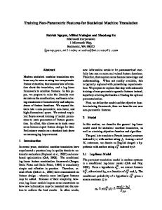
FIG. 1. The rescaled correlator of conductance peak heights ~s! obtained from the Hermitian random matrix simulations ~unitary ensemble!. For comparison, the inset also shows the large-x asymptotics in the correlator of decay widths (n). The solid lines are the analytical predictions for the asymptotic behaviors ~when known! and the dashed line corresponds to the fitted curve c g (x)50.735( p x) 22 . Statistical error bars are too small to be seen. The arrow indicates the correlation width at half maximum height.

We remark that this correlator is not directly accessible to experiments in quantum dots ~recall that conductance peak widths are dominated by the thermal rounding of the Fermi surface!.37 Here we have introduced it with the unique purpose of checking the reliability of the numerical simulations in the x@1 range. Contrary to the situation for c g (x), both x!1 and x@1 asymptotic limits of the rescaled c G (x)5C G (X)/C G (0) can be evaluated analytically. One finds that ~see Appendix B! c G~ x ! →

H

122 p 2 x 2 /3

for x!1

1/~ p x !

for x@1.

2

~2.28!

The data obtained from the random matrix simulations indicate that the asymptotic tail of c g (x) is well described by an x 22 law. In the light of Eq. ~2.28!, this is not very surprising: If one lead were more strongly coupled to the cavity than the other, say, G R @G L , we would have that c g (x)5c G (x)1O(G L /G R ) and therefore c g (x@1);x 22 in leading order. We cannot rigorously prove, though, that this asymptotic form is also exact when right and left leads are identical. To conclude this subsection, we briefly discuss the universality class of preserved TR without spin-orbit coupling ~the case when spin-orbit coupling is present, the symplectic ensemble, will not be discussed since it is not relevant to semiconductor heterostructures!. The simplest experimental realization is a measurement of the evolution of conductance peak heights as a function of shape deformation in the absence of a magnetic field. The general approach is the same as above and we assume that the system Hamiltonian can be modeled as a member of the Gaussian orthogonal ensemble ~GOE!.31 However, the x!1 asymptotics of the conductance peak correlator is now more difficult to calculate. This is not a daunting problem because, as seen above, the numerical results reliably recover the correct behavior of the correlator

53

9973

PARAMETRIC CONDUCTANCE CORRELATION FOR . . .

FIG. 2. The rescaled correlators of conductance peak heights and decay widths from real random matrix simulations ~orthogonal ensemble!, following the same conventions as Fig. 1. The dashed line corresponds to the fitting c g (x)51.214( p x) 22 and the solid line is the theoretical prediction for the x@1 asymptotics of c G (x).

for small values of x. Consequently, for the TR-preserved case we relied entirely on numerical simulations and did not attempt any analytical calculation. We used the same parametric dependence of H(X), but this time drew H 1 and H 2 from the GOE. All other steps were identical to the GUE simulation. The resulting correlation functions ~after the proper rescalings! are shown in Fig. 2. Notice that the largex asymptotics of both c g (x) and c G (x) are well described by an x 22 law, as for the GUE simulations. Here, analogously to the GUE, we do not know how to prove analytically that this decay is rigorously true for c g (x); on the other hand, we do know that this power law decay is indeed exact for c G (x). 38 We emphasize that the most important characteristic of the TR-preserved, universal c g (x) as compared to the TRbroken one is the larger decay width. The widths at half maximum height differ by approximately 20%. The power spectra of conductance peak height oscillations @the Fourier transform of c g (x)# for both GUE and GOE are shown in Fig. 3. Notice that the behavior is exponential only over a small range of k values. One then concludes that a Lorentzian can only be used as a rough approximation to the exact curves. Besides, a Lorentzian cannot accommodate simultaneously the small and large asymptotic limits of c g (x) presented above in either the TR-preserved or TR-broken case. B. The joint distribution of conductance peak heights and their first parametric derivative „unitary ensemble…

In this subsection we evaluate the joint probability distribution

K

S

dg n ~ x¯ ! Q ~ g,h ! 5 d „g2g n ~ x¯ ! …d h2 dx¯

DL

,

~2.29!

where x¯ 5 AC v (0)X¯ and the Hamiltonian belongs to the GUE. This distribution, although not suitable for direct experimental investigations, allows one to easily evaluate higher moments of the conductance peak height and its first

FIG. 3. The Fourier transform of the correlator of peak heights for the GUE ~s! and GOE (n) ensembles. The dashed line is the curve f (k)50.125e 2k/2.75 representing the Fourier transform of a Lorentzian fitted to the GUE data.

parametric derivative; in particular, one can use Q(g,h) to obtain the two first coefficients in the expansion of Eq. ~2.9!, C g~ 0 ! 5

E E `

dg

`

2`

0

~2.30!

dh g 2 Q ~ g,h !

and C 9g ~ 0 ! 52

1 C v~ 0 !

E E `

dg

0

`

2`

dh h 2 Q ~ g,h ! .

~2.31!

We begin by recalling Eq. ~2.6! and introducing the coefficients L n into Eq. ~2.29!,

KS

Q ~ g,h ! 5 d g2

D

L

~2.32!

G

~2.33!

G RnG Ln d ~ h2M n ! , G R n 1G L n

where M n 5 AC v ~ 0 !

F

LL L R 1L L LR 1 2 . G R n G L n G R n 1G L n

Taking the Fourier transform of Eq. ~2.32! with respect to h, we get

KS

˜ ~ g,t ! 5 d g2 Q

L

D

G RnG Ln exp~ itM n ! . G R n 1G L n

~2.34!

Following the same assumptions of the previous subsection, we break up the ensemble average into four partial averages. Recalling Eqs. ~2.13! and ~2.14!, we first carry out the average over the perturbation U:

S

^ exp~ itM n ! & U 5 ) exp 2 mÞn

U

g 4 t 2 D 2 g R*n g R m « n2 m

G R2 n

1

UD

g R*n g L m 2 . G L2 n ~2.35!

9974

BRUUS, LEWENKOPF, AND MUCCIOLO

Next, we evaluate the average over the decay widths

$ g R m , g L m % for m Þ n only,

K S

exp 2

U

g 4 t 2 D 2 g R*n g R m « n2 m

G R2 n

F

5 11

U DL S DG

g L*n g L m G L2 n

1

g 4t 2D 2^ G & « n2 m

2

1 G R3 n

1

21

. ~2.36!

G L3 n

At this point, instead of also taking the average over the remaining decay widths, we consider first the average over the eigenvalues $ « n % , n 51, . . . ,N. Here we use the following relation, valid in the large-N limit and for « n at the center of the spectrum:39

K) F

11

mÞn

~ kD/2p ! 2

« n2 m

GL 21

5B˜ ~ k ! ,

~2.37!

$«n%

where B˜ (k) is the Fourier transform of B~ s !5

35114s 2 13s 4 . 12p ~ 11s 2 ! 4

~2.38!

@The evaluation of the average in Eq. ~2.37! requires a generalization40 of the approach used to derive Eq. ~2.22!. A brief description is given in Appendix C.# After inserting ~2.37! into Eq. ~2.36! and inverse Fourier transforming the result we get

KS S

Q ~ g,h ! 5 d g2

3B

D

1 G RnG Ln 23 2 G R n 1G L n 2 p g A^ G & AG R23 n 1G L n h

2pg

2

A^ G & AG R23n 1G L23n

DL

,

~2.39!

$ G R n ,G L n %

which is more conveniently expressed in the form Q ~ g,h ! 5

e 24g/ ^ G & 2p^G&

2

Ag/ ^ G &

H g/ ^ G &

S

h/ ^ G &

2 p Ag/ ^ G &

D

E aE `

d

0

R

S

d p2 3

Ap

3

`

0

D

23 ~ a 23 R 1aL !

B

S

q

Ap

3

23 ~ a 23 R 1aL !

D

.

~2.41!

In fact, one can easily carry out one of the above integrations and arrive at H p ~ q ! 52p

E

`

0

du e 2 pu

u14

Au ~ u11 !

SA D

B q

~ 35/6p !

for p→0

~ 70/3! Ap/ p

for p→`,

u14 . u11

~2.42!

It is possible to represent H p (q) in terms of special functions, but we did not find it particularly clarifying and there-

~2.43!

whereas for a fixed pÞ0, we have that H p ~ q ! ;O ~ q 24 !

~2.44!

for q@1.

Notice that Eqs. ~2.40! and ~2.42! together immediately lead to the same x!1 asymptotics for the peak height correlator shown in Eq. ~2.25!. From Eq. ~2.44! it is obvious that ^ h n & diverges for n.2. This can be ultimately related to the level repulsion present in the spectrum: Strong anticrossings of levels can cause anomalously large variations of the conductance peak height as a function of the external parameter X. When this happens, one finds that h;1/v , where v 5 u « n 11 2« n u /D!1. Since the probability of this event goes as P( v ); v 2 for the unitary ensemble,31 one finds that Q(g,h);1/h 4 for h@1, in agreement with our exact calculation. III. DYNAMICAL MODEL

The aim of this section is to compare the results of the previous section with exact numerical diagonalizations of a dynamical model. The essential characteristic of a dynamical model for this type of study is a fair resemblance to the actual experimental conditions, combined with its adequacy to numerical computations. For this reason we chose the ~two-dimensional! conformal billiard penetrated by an infinitely thin Aharonov-Bohm flux line carrying a flux of f . This model was originally introduced in Ref. 41 and later adopted in the study of statistical features of conductance in quantum dots.12 Using complex coordinates, the shape of the billiard in the w plane is given by u z u 51 in the following area preserving conformal mapping: w~ z !5

d a L e 2 ~ a R 1 a L 24p !

a Ra L a R1 a L

H

~2.40!

.

The remaining average over the reduced widths a R 5G R n / ^ G & and a L 5G L n / ^ G & appears only in the evaluation of the bell-shaped function H p~ q ! 5

fore do not do it here. The asymptotic limits follow directly from the integral representation shown above. For q50, we obtain H p~ 0 ! →

$gm%

1

53

z1bz 2 1ce i d z 3

A112b 2 13c 2

~3.1!

,

where b, c, and d are real parameters chosen in such a manner that u w 8 (z) u .0 for u z u <1. The classical dynamics of a particle bouncing inside this billiard is predominantly stochastic and is unaffected by the presence of the flux line. To describe the flux line we chose the following gauge for the vector potential A: A~ w ! 5

S

f ] f ~w! ] f ~w! ,2 ,0 2 p ] Im~ w ! ] Re~ w !

D

~3.2!

where f (w)5ln@uz(w)u#. This particular gauge, combined with Neumann boundary conditions, permits a separation of the Schro¨dinger equation into polar coordinates (r, u ) of the complex parameter z5re i u . The eigenstates c n thus obtained correspond to the resonant wave function appearing in Eq. ~2.3!.12 In our numerical treatment the wave function x c in the lead is equal to a transverse sine function multiplied by a longitudinal plane wave.

53

PARAMETRIC CONDUCTANCE CORRELATION FOR . . .

In practical calculations,12 one fixes the value of the flux f and uses as a truncated basis the lowest ~in our case 1000! eigenstates of the circular billiard (b5c50). These have the form J n ( g n n r)e il u , where J n is the Bessel function of fractional order n and g n n is the nth root of its derivative, J 8n ( g n n )50. The dependence on the magnetic flux enters through n 5 u l2 f / f 0 u , with f 0 as the flux quantum h/e. To solve the Schro¨dinger equation one has to calculate several thousand matrix elements of the Jacobian J 5 u w 8 (z) u 2 in this f -dependent basis. This operation is very time consuming. Changes in shape are not a major obstacle, since b, c, and d act as prefactors to the matrix elements and no further calculation is necessary. ~For instance, in Ref. 12 only two different values of f needed to be used.! In the present work, however, we wanted to change the flux to simulate the simplest experimental setup and this required the use of 76 different values of f . The spectrum is seen to be not only 2 p periodic in f , but also symmetric around f / f 0 51/2. For this reason and, furthermore, to avoid the special points 0 and 1/2 we let f / f 0 vary in the interval @ 0.1,0.4# . To circumvent the overwhelming problem of too large amounts of computing time we employed the following strategy. We calculated the Jacobian matrix J for only seven different values of a 5 f / f 0 , namely, from 0.10 to 0.40 in steps of 0.04. Then, for any other value of a , the matrix element J i j ( a ) was found by polynomial interpolation. This was checked to give a relative error of at most 1027 . To improve the statistics we also calculated the eigenstates for five different shapes by keeping b5c50.2 and letting d 5k p /6, with k51,2,3,4,5. The spectra corresponding to these shapes are statistically uncorrelated.12 Due to the truncation of the basis only the lowest 300 of the calculated 1000 eigenstates were accurate enough to be used in the analysis. We also discarded the lowest 100 eigenstates because of their markedly nonuniversal behavior. We should emphasize that it is not a trivial task to increase the number of usable states. For the asymmetric conformal billiard no symmetry reduction of the resulting eigenvalue problem is possible. The presence of the flux line constrains the method of analysis to the diagonalization of large Hermitian matrices, limiting the number of eigenstates that can be treated efficiently.

9975

FIG. 4. The level velocity correlation function for the conformal billiard ~s! averaged over five shapes, 76 values of the flux, and 200 energy levels. The full line is the result of the GUE simulation.

Sec. II. The position of the leads and their widths were specified in the following way. Based on autocorrelation calculations of the eigenfunction c n along the perimeter of the billiard, we found that the spatial decorrelation for the relevant levels ~levels 201 to 300! takes place over a distance around 1/60 of the perimeter. We therefore decided to take the width of the leads to be 1/24 of the perimeter, i.e., 2.5 times the decorrelation length, yielding 24 adjacent leads. To improve the statistics we used all 24 lead position for each c n . Due to the relatively large width of the leads, adjacent leads are not correlated, as was verified by obtaining the same result ~with larger fluctuations! using only every second or every third lead. The result of the calculation is shown in Fig. 5. A fair agreement with Eq. ~2.28! is noted. Finally, we calculated the conductance peak correlation c g (x), Eq. ~2.7!, for the conformal billiard using the abovementioned decay widths. We chose all possible pair configurations among the 24 lead positions. The result is shown in Fig. 6 and, again, a fair agreement with the predictions of Sec. II A is observed. Notice that the data for the conformal billiard are not fully consistent with a Lorentzian if we fix the x!1 asymptotics of the curve to be identical to Eq.

A. Correlation functions for the billiard

In the following, we present the numerical results for the correlators of level velocity, decay widths, and conductance peak heights. ~Recall that at present only the last can be directly measured in real experiments.! Figure 4 shows the level velocity correlator defined by Eq. ~2.23! rescaled according to c v (x)5C v (x)/C v (0), with x5 a / AC v (0). The plotted data were obtained by averaging over 76 equidistant values of a in the interval @ 0.1,0.4# , over the eigenstates between 201 and 300, and over the five different shapes mentioned above. We observe a good agreement with the analytical results33 for small values of x and with random matrix simulations in general. A thorough discussion of the scaling factor AC v (0) dependence on energy and billiard shape is postponed to the next subsection. Next we employed the billiard model to obtain the decay width autocorrelation function c G (x), Eq. ~2.27!. The decay widths G k n for the billiard were calculated as described in

FIG. 5. The decay width correlation function for the conformal billiard ~s! for a fixed shape (b5c50.2 and d 5 p /3) and averaged over 76 values of flux and 200 energy levels. The full line is the result of the GUE simulation.

9976

53

BRUUS, LEWENKOPF, AND MUCCIOLO

FIG. 6. The peak height correlation function for the conformal billiard ~s! for a fixed shape (b5c50.2 and d 5 p /3) averaged over 76 values of flux and 200 energy levels. The full line is the result of the GUE simulation.

~2.25!. A squared Lorentzian does not seem to provide a better approximation either, although in a recent experiment19 c g (x) was measured and such a curve was fitted to the data. It would be interesting to check how well our result for c g (x) based on random matrix calculations matches the available experimental data without any fitting parameter ~in Sec. III B we will present a way to predict the typical field correlation scale!. For all three correlators we have noticed large statistical fluctuations between data taken at different billiard shapes. We found that most levels around the 300th one ~the upper limit of reliability in our calculation! still do not show more than one full oscillation within the range of flux allowed by symmetry. The averaging over shape deformation was thus crucial to get rid of the remaining nonuniversal features. After averaging over the five values of d mentioned previously ~see also the following subsection!, we found that C v (0) near the Nth level obeys the law C v (0)'1.202AN. We ascribe the small mismatch between theory and numerics, particularly at x.1, to poor statistics. As mentioned before, the only way to circumvent this problem is to compute higher eigenstates. Fortunately, this difficulty does not appear in real experiments where the magnetic flux is extended over the whole area of the cavity and the dependence of f is not periodic. B. Energy dependence of C v „0… for billiards

One of the important features of a dynamical model is that its quantum fluctuations display a marked dependence on energy. A quantitative understanding of the field scale of the fluctuations and its dependence on energy is important to put any random matrix result in contact with measurements in quantum dots. For this purpose, the semiclassical approach can be used in a relatively simple form. The aim of this subsection is to discuss the energy dependence of the level velocity correlator C v (0), which is a measure of the quantum fluctuations, and show that one can successfully estimate this quantity using exclusively classical quantities. It was already properly noticed by Berry and Robnik41 that the typical flux necessary to induce a crossover

from GOE- to GUE-like spectral fluctuations in a chaotic billiard threaded by an Aharonov-Bohm flux line scales with the energy as E 1/4. The origin of this dependence has a simple semiclassical explanation which was nicely worked out by Ozo´rio de Almeida and co-workers.43,44 The nonuniversal scaling C v (0) can be obtained in an analogous manner. Our point of departure is a recent work by Berry and Keating42 based on the Gutzwiller trace formula. Most of our semiclassical considerations follow their findings. However, our interpretation and the method we use to quantify C v (0) are different. To make the exposition self-contained, we shall briefly describe points of their work which are relevant to our discussion and comment when necessary. The initial step is to approximate C v ( f ) by a two-point correlator. ~The nature of the approximation is evident, since to track down the parametric evolution of a single eigenvalue for any f is a task that cannot be exactly achieved by considering only Green’s functions with a finite number of points.! As in Ref. 42, we write 1 F h ~ f ,E ! 5 ¯ df

E

d f¯

K S D S DL

d f¯

d f ¯2 N f h 2 d f¯

f d 3 ¯ N h f¯ 1 2 df

,

~3.3!

dE

where N h (E, f )5 ( n Q h „E2« n ( f )… is a smoothed cumulative level density which counts the number of single-particle states up to an energy E at a magnetic flux f . For the smoothing it is convenient to adopt the form dQ h (E)/dE[Im(E2i h ) 21 / p , where the parameter h is chosen to be much smaller than D. ~We would like to point out a change in notation: Throughout this subsection angular brackets ^ ••• & will denote energy averages in distinction to the previous ensemble averages.! The energy average in Eq. ~3.3! is taken over a range d E around E. Ordinarily, the average over the magnetic flux is taken over a window d f¯ in flux which corresponds to little change in the classical dynamics but is semiclassically large, i.e., it corresponds to sizable fluctuations in the spectrum. For billiards threaded by Aharonov-Bohm flux lines this is not an actual constraint, since flux variations have no effect on classical trajectories. Nonetheless, when considering the correlator of Eq. ~3.3! one has, in principle, to avoid f¯ pertaining to the TRbreaking crossover regime. When levels are much farther apart than h , it is straightforward to show that dN h ( f¯ )/d f¯ can be approximated by D 21 d« n ( f¯ )/d f¯ . For f larger than a certain f c such that the correlation between level velocities of different states m Þ n is much weaker than for m 5 n , F h ( f ,E) is equivalent to C v ( f ) and independent of h , provided that the energy levels are taken to be within d E. This equivalence also holds in the limit of f 50 when the spectrum is nondegenerate. In summary, F h (E, f ) is a good approximation to the level velocity correlator C v ( f ) only for f 50 and f . f c . In fact, F h (E, f ) is also the quantity evaluated analytically by Szafer and Altshuler32 in the context of disordered metallic rings, using a diagrammatic perturbation theory based on impurity averaging.

53

9977

PARAMETRIC CONDUCTANCE CORRELATION FOR . . .

Following Ref. 42, we now turn to the semiclassical treatment. In particular, we specialize the results to billiards threaded by a flux line. This simplifies the problem enormously since if S n is the action of a periodic orbit n, upon applying a magnetic flux f we find that S n →S n 12 p \w n f / f 0 , where w n is the number of times the orbit n winds around the flux line. The cumulative level density is expressed semiclassically using the Gutzwiller trace formula and one writes the correlator as F h ~ f ,E ! 5

S D K( 2p f0

HS J L

2

12 p w n

nm

u A m A n u w 2n exp i

D

S n 2S m \

f h ~ T n 1T m ! 2 d wnwm f0 \

~3.4!

, dE

where the amplitudes A n (E) contain information on the stability of the orbit n as well as its Maslov index. The smoothing of the staircase function gives rise to the exponential damping factor h times T n (E), the period of the closed orbit n. In the semiclassical limit, N(E)@1, the flux range of the TR-breaking crossover is much smaller than f 0 . Therefore, without affecting considerably the calculation for the pure TR-broken case, we take the limit of d f¯ → f 0 . Now one arrives at one of the delicate points of the semiclassical approach. The correlator F h ( f ,E) is expressed as a sum of diagonal and off-diagonal contributions. In contrast to the fact that it is a settled matter how to compute the diagonal part, the evaluation of the off-diagonal term is still an unsatisfactorily solved problem. It seems that for F h it is reasonable42 to neglect the off-diagonal contribution and we will do so hereafter. The diagonal part of F h ( f ,E) in Eq. ~3.4! is still difficult to evaluate since, in principle, it requires the knowledge of the full set of periodic orbits up to the cutoff \/ h . This can be simplified by the following considerations. For chaotic systems, the number of periodic orbits grows exponentially as a function of their length L and ergodicity ensures that as the orbits become longer they tend to explore the phase space more uniformly. Thus, one can define a critical length L c corresponding to a uniform coverage of the phase space by the periodic trajectories. For a fixed energy E, L c determines T c , the time when the Hannay and Ozo´rio de Almeida sum rule45 is applicable, allowing the sum over periodic orbits to be calculated as an integral over orbital times. Applying this sum rule to the diagonal part of Eq. ~3.4! one obtains F hdiag~ f ,E ! '

2

f 20

E

` dT

Tc

S

T

3exp 2

S

w 2 ~ T ! cos 2 p w ~ T !

D

2hT . \

f f0

D ~3.5!

Here the overbar stands for an average over the phase space, or, in practice, over an ensemble of trajectories. The replacement of the summation over periodic orbits by an average over trajectories makes the problem amenable for a computational evaluation of F hdiag( f ,E). Such a procedure has already been successfully used to estimate the GOE to GUE transition parameter in the stadium billiard.46

FIG. 7. Numerical estimate of the winding number variance w 2 as a function of orbit time T in the classical billiard with unit area, v F 51, and d 5 p /3.

By writing the winding number as an integral over the angular velocity, w(T)5 * T0 dt u˙ (t)/2p , it is simple to see that for an ergodic system w(T)50. The winding number variance is given by w 2~ T ! 5

1 ~ 2p !2

E E T

T

dt

0

0

dt 8 C ~ t 8 2t ! '

T ~ 2p !2

E

`

0

dt 8 C ~ t 8 ! , ~3.6!

where C(t)5 u˙ (t 8 ) u˙ (t 8 1t). For chaotic systems in general the correlator C(t) decays sufficiently fast in T to assure the convergence of the integral in Eq. ~3.6!.47 The knowledge of the winding number distribution P(w,T) allowed us to evaluate the phase space average in Eq. ~3.5!. To determine P(w,T) for the conformal billiard we have randomly chosen 104 initial conditions and computed trajectories up to 250 bounces for the particular deformation b5c50.2 and different d ’s. We have generated a histogram recording w and T every time a trajectory winds around the flux line located at the origin.48 The results displayed in Fig. 7 confirm Eq. ~3.6!. The variance of w(T) is better written as46 w 2~ T ! 5 k

S D 2E mA

1/2

~3.7!

T,

where A is the billiard area and k is a system-dependent quantity computed for the scaled billiard with unit area and trajectories with unit velocity. Moreover, our numerical results give us confidence that for any given time P(w,T) is a Gaussian distribution ~see Fig. 8!. This is in agreement with the conjecture of Ref. 41 for periodic orbits. Substituting this result into ~3.5! and bearing in mind that in the semiclassical limit h T c /\!1, for f 50 we obtain F hdiag~ 0,E ! '

1

f 2c

Using the leading term in N(E)'AmE/2p \ 2 , we can write

f c5

the

f0 . @ 4 p k N ~ E !# 1/4 2

~3.8!

. Weyl

formula,

~3.9!

9978

BRUUS, LEWENKOPF, AND MUCCIOLO

FIG. 8. The distribution of winding numbers ~solid line! for T5150 in the classical billiard with unit area, v F 51, and d 5 p /3. The dotted line is a Gaussian curve with variance given by Eq. ~3.7!.

Notice that f c ! f 0 . Although F( f ,E) fails as an accurate approximation for C v ( f ) over the entire range of f , we expect it to work for f 50 and f @ f c . Therefore the semiclassical quantity f c given above should yield a good approximation to the exact inverse field scale AC v (0). We used the same procedure described to obtain P(w,T) to compute k as a function of d . The results are shown in Fig. 9. Figure 10 shows C v (0) as a function of N from quantum mechanical ~Sec. III A! and semiclassical ( f 22 c ) calculations. From the numerical diagonalizations we found that the proportionality factor between C v (0) and N 1/2 varies between 0.94 ( d 55 p /6) and 1.54 ( d 5 p /6), while the semiclassical estimate gives 0.90 for d 5 p /2, for instance. Clearly, both quantum and semiclassical calculations indicate that C v (0) depends on the billiard shape. When comparing the results of these two calculations, one should also note the size of the large fluctuations in the data presented in Fig. 10. As already remarked in the previous subsection, these large statistical fluctuations are due to the limited data set used in the simulations. To put the semiclassical result in direct contact with experiments, one needs some system-specific information to

53

FIG. 10. C v (0) as a function of AN for the conformal billiard, with N as the eigenstate number. The symbols indicate the data obtained from the exact numerical diagonalization ~fully quantum! for different geometries. The solid line is the total average over all data: C v (0)51.202AN. The dashed and dotted lines are the semiclassical estimates @Eq. ~3.8!# for d 5 p /2 ( k 50.253) and d 5 p /3 ( k 50.314), respectively.

compute k . In the above discussion, k gives a measure of how fast the winding number variance increases with time. For the more physical situation of extended B fields, k measures the rate of increase in the variance of accumulated areas as a function of time.43 It is interesting to notice that the semiclassical interpretation of the scales of the conductance autocorrelation function for quantum dots and open cavities is very similar. Since quantum dots have G!D, the escape time \/G is always semiclassically large. In this regime, the physics is dominated by the classical decorrelation time t implied in Eq. ~3.6!. The situation is very different for open cavities, where the escape time plays an important role, since it is comparable with t . For the quarter stadium and extended B fields, Ref. 46 gives k '0.3. In this study we observed that k is a relatively robust number, since very different shapes of the conformal billiard give values of k that differ at most by 60%. Therefore we believe that with help of Eq. ~3.9! and taking k to be of order unity, one can estimate the magnitude of f c for other chaotic billiards. IV. CONCLUSIONS AND DISCUSSION

FIG. 9. The numerical coefficient k as a function of geometry for the classical conformal billiard.

In this paper, we have proposed that the universal form of the parametric correlator of conductance peak heights indicates the chaotic nature of the electron dynamics in quantum dots in the Coulomb blockade regime. In experiments, the simplest parameter to vary is an external magnetic field. Whereas random matrix theory provides the universal form of the correlation function, the nonuniversal field scale can be understood in simple semiclassical terms: it is related to the average winding number per unit of time of periodic orbits bouncing between the confining walls of the quantum dot. This field scale is rather sensitive to the geometry of the dot and the Fermi energy. To compare our analytical and numerical predictions against the experimental result, the magnetic flux through the dot has to be larger than one quantum unit of flux h/e, but such that the cyclotron radius is much larger than the dot diameter. The former condition as-

53

9979

PARAMETRIC CONDUCTANCE CORRELATION FOR . . .

sures that time-reversal symmetry is broken; the latter implies that the bending of classical trajectories is mainly due to scattering by the boundaries. We point out that electronelectron correlations can be taken into account by assuming that the single-particle spectrum results from a selfconsistent ~Hartree-Fock! treatment.49 Our theoretical prediction for the correlator of peak heights is based on the hypothesis that the statistical properties of the system Hamiltonian can be described by random matrix theory. Although we could only derive analytically expressions for the limit of small field variations, the complete form of the correlation function was obtained by numerical simulations of large Gaussian matrices. We have compared the random matrix results with the exact correlator obtained from the conformal billiard after averaging over energy and shape deformation. The agreement found was good, given the limitations imposed by the size of the data set. In addition to that, we found that the result of the classical calculation for the magnitude of the field scale and its dependence on energy matches the quantum result moderately well. For experimental tests of our theory, it is important to note that dephasing in the small quantum dot has to be kept low enough, namely, the dephasing length has to be larger than the system size. Also, the parametric results presented for the GUE case were illustrated in a dynamical model in which only the magnetic field was varied. This was very convenient, since it allowed us to relate the field scaling parameter to the underlying classical dynamics using a well-developed formalism. Alternatively, the external parameter could be taken as the shape variation. For B50, the conductance autocorrelation function should then follow our numerical results for the GOE case. Or, by varying the shape with B.B crossover , the conductance peak correlator should be given by our GUE results. ~While finishing this work we learned that such an experiment has already been performed.19! Unfortunately, the semiclassical analysis for these situations is more difficult than the one presented here and still remains an open problem. Some billiard geometries have well-pronounced short periodic orbits which, for insufficient averaging over energy and magnetic field, can lead to strong nonuniversal features to the curves presented in this work. We believe that overcoming this problem will be one of the most serious challenges for the experiments. In particular, to verify experimentally the asymptotic behavior of c g (x) should be very difficult. Since c g (x) involves the subtraction of two numbers and for x@1 these numbers become very close, statistical ~nonuniversal! fluctuations can easily drive the experimental c g (x) below zero. Another cause of deviations from the predicted universal behavior, presumably weaker, is the existence of wave function correlations which extend over the dot. In other words, our findings assume that the channels at different leads are decorrelated, which may not be completely true if the dot size is not much larger than the electron wavelength. The agreement of our random matrix results with the numerical calculations using the conformal billiard supports the assumption of independent channels for N.200. Smaller systems should be more influenced by short or direct orbit effects. We should also mention that if there were strong correlations between heights of neighboring

peaks of a given sequence, they would influence mostly the x@1 region of the correlator. This is because averaging over a finite range of magnetic field usually yields less statistics for large field differences and, consequently, more pronounced data correlation effects. Lastly, we point out the fact that, independently of previous considerations, another very interesting experiment is a direct measurement of c v (x). Despite the very large Coulomb energy, which makes the conductance peak spacing very regular at first sight, a careful experiment should be able to observe the small fluctuations of the peak position as a function of an applied magnetic field. This will give direct information about the single-particle level dispersion or, equivalently, c v (x). It will also provide a direct test of our estimate of the flux correlation scale f c . Note added. After the submission of this manuscript we learned of similar work by Alhassid et al.54 ACKNOWLEDGMENTS

H.B. was supported by the European Commission under Grant No. ERBCHBGCT 930511. C.H.L. acknowledges the financial support of the National Science Foundation. Both H.B. and C.H.L. thank NORDITA for its hospitality. We are grateful to B. Altshuler, O. Klein, C. Marcus, B. Simons, N. Taniguchi, and S. Tomsovic for helpful discussions and to R. Jalabert for suggestions concerning the manuscript. We also thank H. Baranger and C. Marcus for providing us with Refs. 16 and 19, respectively, prior to publication. APPENDIX A: EVALUATION OF Šdet„H 2 …tr„H 22 …‹ H

This appendix is devoted to a rather detailed evaluation of the average over the determinant shown in Eq. ~2.20!. Let us call c N 5 ^ det~ H 2 ! tr~ H 22 ! & H ,

~A1!

where H is now an N3N GUE matrix. First, we notice that there is a more convenient way to express this average, namely, c N5

d f ~a! da

U

~A2!

, a50

where the generating function f (a)5 ^ det(H 2 1a1N ) & H can be evaluated by the fermionic method:36 f ~ a ! 5 ^ det~ H1 a 1N ! det~ H2 a 1N ! & H 5

KE

d @ x # exp@ 2 x † ~ H ^ 12 1 a 1N ^ L ! x #

L

,

~A3!

H

where a52 a 2 , L5 diag(1,21), and x T 5( x T1 , x T2 ), with x 1 and x 2 representing N-component fermionic vectors. Averaging over the GUE matrix H we find that

F

^ exp~ 2 x † H ^ 12 x ! & H 5exp 2 where u is the following 232 matrix:

G

l2 tr~ u 2 ! , 2N

~A4!

9980

BRUUS, LEWENKOPF, AND MUCCIOLO

u5

S

x †1 x 1

x †2 x 1

x †1 x 2

x †2 x 2

D

The quartic term can be decoupled by a HubbardStratonovich transformation, namely,

E

F

d @ Q # exp 2

N tr~ Q 2 ! 2il tr~ Qu ! 2 5

G

S D F 2p N

2

exp 2

G

l2 tr~ u 2 ! , ~A6! 2N

S DE

3

E

2

F

N d @ Q # exp 2 tr~ Q 2 ! 2

and

G

S DE J

H

d @ Q # exp 2

N tr~ Q 2 ! 1N tr@ ln~ a L 2 ~A8!

1ilQ !# .

When N@1 the above integral over Q can be evaluated by the saddle-point approximation ~which becomes exact in the limit N→`). For this purpose we first separate angular and radial components of Q, namely, Q5T † qT, where q5 diag(q 1 ,q 2 ) and T is an SU~2! matrix. The differential breaks up into d @ Q # 5d m (T)J(q)d @ q # , where J(q)5 p (q 1 2q 2 ) 2 is the Jacobian of the transformation, d @ q # 5dq 1 dq 2 , and d m (T) is the group measure normalized to unity. This yields

S DE

N f ~ a !5 2p 3

E

d @ q # J ~ q ! exp~ 2NF @ q # !

G

iaN tr~ q 21 TLT † ! , d m ~ T ! exp 2 l

~A9!

where F @ q # 5(1/2) tr(q 2 )2 tr@ ln(ilq)# and we have only kept terms to lowest order in a . The saddle-point expansion now involves only the radial part of the action: F @ q # 5122ln~ l ! 2

d m ~ T ! exp@ b tr~ LTLT † !# 5

G

i a s 1N tr~ LTLT † ! . l ~A11!

det@ exp~ b l i l j !# , b ~ l 1 2l 2 ! 2

~A12!

with l 1,2 denoting the eigenvalues of L. Hence, f ~ a ! 52N

S D l2 e

N

sin~ 2 a N/l ! ~ 2 a N/l !

~A13!

ip ~ s 1 1 s 2 ! 1 d q 21 1 d q 22 1O ~ d q 3 ! , 2 ~A10!

where q 1,25 s 1,21 d q 1,2 and s 21,251. The relevant saddle points correspond to s 1 52 s 2 , resulting in

N

~A14!

.

APPENDIX B: THE ASYMPTOTIC LIMITS OF C G „X…

The small-X asymptotics of the correlator of decay widths can be determined by the same method used in Sec. II A for the conductance peak height correlator. Beginning with the definition presented in Eq. ~2.27!, we expand G k n (X¯ 6X/2) up to first order in X @see Eq. ~2.5!#. The zeroth-order term of C G (X) is then given by C G ~ 0 ! 5 ^ G 2n & 2 ^ G n & 2 5 ^ G & 2

~B1!

for the unitary ensemble. An expression analogous to Eq. ~2.8! is used to write the second-order coefficient of C G (X) in terms of the amplitudes L n , namely, 1 C G9 ~ 0 ! 52 ^ L 2n & . 2

~B2!

Carrying out the average over the matrix elements of the external perturbation U @see Eq. ~2.13!#, we find that C G9 ~ 0 ! 52

2

F

d m ~ T ! exp 2

S D

d @ x # exp@ 2 x † ~ a 1N ^ L1il1N ^ Q ! x # .

2

F

N

4N 3 l 2 c N5 2 3l e

The Gaussian integral over the fermionic variables can be easily carried out, yielding N 2p

l2 e

~the factor of 2 takes into account the double saddle point!. Finally, we obtain

~A7!

f ~ a !5

S DE

The integral over the SU~2! manifold can be evaluated through the well-known Itzykson-Zuber formula,50 which in a simplified form reads

E

where Q is a 232 Hermitian matrix d @ Q # 5dQ 11dQ 22dQ 12dQ 21 . As a result, we have N f ~ a !5 2p

f ~ a ! 5N

~A5!

.

53

s2 N

K(

mÞn

G nG m « n2 m

L

.

~B3!

We now average separately over the eigenvalues and partial widths and obtain C G9 ~ 0 ! 52

2 p 2^ G & 2s 2X 2 . 3ND 2

~B4!

Upon rescaling both C G (X)→c G (x)5C G (X)/ ^ G & 2 and X→x5X( s 2 /ND 2 ), we arrive at c G ~ x ! 512

2 p 2x 2 1O ~ x 4 ! . 3

~B5!

The large-X asymptotics of C G (X) can be inferred from the asymptotics of another correlator, namely,

53

9981

PARAMETRIC CONDUCTANCE CORRELATION FOR . . .

P ~ X,E ! 5V 2

K(

m,n

and

u c m ~ r;X 1 ! u 2 u c n ~ r;X 2 ! u 2 d „E 1

L

2« m ~ X 1 ! …d „E 2 2« n ~ X 2 ! … 2

n ~ v ,x ! 5

1 D2

~B6!

where V is the system volume, X 1,25X¯ 7X/2, and E 1,25E¯ 7E/2. Recall that the wave function intensities are proportional to the decay widths G m (X 1 ) and G n (X 2 ) for pointlike contacts. At E 1 5E 2 and large X, the interlevel correlations are secondary to intralevel ones; as a result, the d function in Eq. ~B6! acts as a Kronecker d , causing P(X,0) and C G (X) to coincide ~up to a prefactor equal to D 2 ) to leading order in O(1/X). Let us for convenience assume a finite size space basis to represent the system Hamiltonian. We can then reduce Eq. ~B6! to

SD

N P ~ X,E ! 5 p

P ~ X,E ! 52

1 D2

~B7!

S D

N2 Re^ @ G ~ E 1 1i e ;X 1 !# kk 2p2 1 . D2

~B8!

In general, an expression like Eq. ~B8! requires the evaluation of the following quantity: D klmn ~ E,X ! 5 ^ @ G ~ E 1 1i e ;X 1 !# kl @ G ~ E 2 2i e ;X 2 !# mn & . ~B9! The correlator D klmn (E,X) can be calculated exactly in the zero-mode approximation of the supersymmetric nonlinear s model51 ~or, equivalently, in the RMT framework!. This calculation is standard nowadays ~for a recent review, see Ref. 52! and has already been presented in the literature.53 Here we will only mention the resulting expression for the unitary ensemble, which is D klmn ~ E,X ! 5

S D p ND

2

@ d kl d mn 2 d kl d mn k ~ v ,x !

2 d kn d lm n ~ v ,x !# ,

~B10!

where

E E 1

1

21

dl 2 exp@ 2 p i ~ v /21i h !~ l 1 2l 2 !

2 ~ p 2 x 2 /2!~ l 21 2l 22 !#

K

P 4j51 det~ H2m j D ! det~ H2i a D ! det~ H1i a D !

~B11!

L

5 H

1

21

dl 2

S

D

l 1 1l 2 exp@ 2 p i ~ v /21i h ! l 1 2l 2

3 ~ l 1 2l 2 ! 2 ~ p 2 x 2 /2!~ l 21 2l 22 !# .

F

~B12!

When writing these equations we have rescaled the variables to E/D5 v , e /D5 h , and ND A tr(U 2 )X/ p 2 5x. Going back to Eq. ~B8!, we arrive at p ~ x, v ! 5D 2 P ~ E,X ! 5

1 Re@ k ~ v ,x ! 1n ~ v ,x !# . 2

~B13!

Since k(0,x)→2/( p x) 4 and n(0,x)→2/( p x) 2 as x→`, we have that p(x,0)→1/( p x) 2 in the same limit. Therefore, we expect that x→`

^ Im@ G ~ E 1 1i e ;X 1 !# kk Im@ G ~ E 2

3 @ G ~ E 2 2i e ;X 2 !# kk & 2

dl 1

1

dl 1

c G ~ x ! ——→

with G(E;X)5 @ E2H(X) # 21 and e →0 1 . The above expression can be rewritten in the more convenient form

`

`

2

2i e ;X 2 !# kk & 2

k ~ v ,x ! 5

E E

1 . ~ px !2

~B14!

Finally, we remark that the x@1 universal asymptotics of both k(0,x) and n(0,x) can also be obtained by the diagrammatic perturbation theory of disordered metals expressed in terms of diffusion modes. APPENDIX C: EVALUATION OF B„s…

In this appendix we give a schematic description of the calculation of B(s). The starting point is Eq. ~2.37!. Here we go through the same steps of Sec. II A to evaluate A « @see Eq. ~2.18!#. First we fix the reference eigenvalue « n to the center of the spectrum, obtaining B˜ ~ k ! 5

1 r~ 0 !

K( ) F N

n 51 m Þ n

d ~ « n ! 11

~ kD/2p ! 2

« n2 m

GL 21

. $«n%

~C1!

Next, we rephrase this expression in terms of an average over a spectral determinant, namely, B˜ ~ k ! 5a N

K

det~ H 4 ! det@ H 1 ~ kD/2p ! 2 # 2

L

~C2!

, H

where a N is a constant @such that B˜ (0)51# and the average is performed over an (N21)3(N21) GUE matrix H. The appearance of determinants in both numerator and denominator in Eq. ~C2! makes its evaluation technically more difficult than Eq. ~A1!. It is necessary to introduce not only four anticommuting auxiliary variables, but also two commuting ~complex! ones. The resulting symmetry group is U(1,1u 4) ~the pseudo-unitarity is due to the structure of the denominator!. Fortunately, a general solution for such graded symmetry problems has been recently worked out.40 The derivation is a nontrivial generalization of the method of Appendix A. For an expression with the structure of Eq. ~C2!, one arrives at the following formula:40

G

Ae 22 p a ~ i a 2m 3 !~ i a 2m 4 ! ~ i a 1m 1 !~ i a 1m 2 ! i p ~ m 1m 2m 2m ! 1 2 3 4 , ~C3! e a $ m j % ~ m 3 2m 1 !~ m 3 2m 2 ! ~ m 4 2m 1 !~ m 4 2m 2 !

(

9982

BRUUS, LEWENKOPF, AND MUCCIOLO

where the sum runs over all six nonequivalent combinations of pairs of m j , a .0, and A is an unspecified constant. To get B˜ (k) we need to take the limit m j →0 for all j51,2,3,4 at a given order. After some algebra, one finds that e 2k B˜ ~ k ! 5 ~ 24124k18k 2 1k 3 ! . 24

1

~C4!

Reviews of experimental and theoretical aspects of quantum chaos in nanostructures can be found in Chaos 3 ~1993!. See also H. U. Baranger, in Nanotechnology, edited by G. Timp ~AIP, New York, in press!; R. M. Westervelt, ibid. 2 R. A. Jalabert, H. U. Baranger, and A. D. Stone, Phys. Rev. Lett. 65, 2442 ~1990!. 3 C. M. Marcus, A. J. Rimberg, R. M. Westervelt, P. F. Hopkins, and A. C. Gossard, Phys. Rev. Lett. 69, 506 ~1992!. 4 M. W. Keller, O. Millo, A. Mittal, D. E. Prober, and R. N. Sacks, Surf. Sci. 305, 501 ~1994!. 5 A. M. Chang, H. U. Baranger, L. N. Pfeiffer, and K. W. West, Phys. Rev. Lett. 73, 2111 ~1994!. 6 M. J. Berry, J. A. Katine, R. M. Westervelt, and A. C. Gossard, Phys. Rev. B 50, 17 721 ~1994!. 7 J. P. Bird, K. Ishibashi, Y. Aoyagi, T. Sugano, and Y. Ochiai, Phys. Rev. B 50, 18 678 ~1994!. 8 For a review, see M. A. Kastner, Rev. Mod. Phys. 64, 849 ~1992!, and references therein. 9 See, for instance, U. Sivan, F. P. Milliken, K. Milkove, S. Rishton, Y. Lee, J. M. Hong, V. Boegli, D. Kern, and M. deFranza, Europhys. Lett. 25, 605 ~1994!. 10 R. A. Jalabert, A. D. Stone, and Y. Alhassid, Phys. Rev. Lett. 68, 3468 ~1992!. 11 V. N. Prigodin, K. B. Efetov, and S. Iida, Phys. Rev. Lett. 71, 1230 ~1993!. 12 H. Bruus and A. D. Stone, Phys. Rev. B 50, 18 275 ~1994!; Physica B 189, 43 ~1993!. 13 E. R. Mucciolo, V. N. Prigodin, and B. L. Altshuler, Phys. Rev. B 51, 1714 ~1995!. 14 Y. Alhassid and C. H. Lewenkopf, Phys. Rev. Lett. 75, 3922 ~1995!. 15 H. U. Baranger and P. A. Mello, Phys. Rev. Lett. 74, 142 ~1994!; R. A. Jalabert, J.-L. Pichard, and C. W. J. Beenakker, Europhys. Lett. 27, 255 ~1994!. 16 A. M. Chang, H. U. Baranger, L. N. Pfeiffer, K. W. West, and T. Y. Chang ~unpublished!. 17 P. M. Brouwer and C. W. J. Beenakker, Phys. Rev. B 51, 7739 ~1995!. 18 O. Klein ~private communication!. 19 J. A. Folk, S. R. Patel, S. F. Godijn, A. G. Hulbers, S. M. Cronenwett, C. M. Marcus, K. Campman, and A. C. Gossard ~unpublished!. 20 I. H. Chan, R. M. Clarke, C. M. Marcus, K. Campman, and A. C. Gossard, Phys. Rev. Lett. 74, 3876 ~1995!. 21 O. Bohigas, in Chaos and Quantum Physics, edited by M.-J. Giannoni, A. Voros, and J. Zinn-Justin ~North-Holland, Amsterdam, 1991!. 22 For classical hyperbolic systems one expects quantum universal behavior in the semiclassical region of the spectrum, i.e., where the electron wavelength at the Fermi surface is small enough to

53

Finally, inverse Fourier transforming the above expression, we arrive at

B~ s !5

E

dk 2iks 35114s 2 13s 4 e B˜ ~ k ! 5 . 12p ~ 11s 2 ! 4 2` 2 p `

~C5!

resolve the typical ‘‘irregularities’’ of the cavity. This is usually the case for two-dimensional systems with more than O(102 ) electrons. 23 R. Landauer, IBM J. Res. Dev. 1, 223 ~1957!. 24 M. Bu¨ttiker, Phys. Rev. Lett. 57, 1761 ~1986!; IBM J. Res. Dev. 32, 317 ~1988!. 25 C. H. Lewenkopf and H. A. Weidenmu¨ller, Ann. Phys. ~N.Y.! 212, 53 ~1991!. 26 A. M. Lane and R. G. Thomas, Rev. Mod. Phys. 30, 257 ~1958!. 27 M. R. Zirnbauer, Nucl. Phys. A560, 95 ~1993!. 28 Y. Meir, N. S. Wingreen, and P. A. Lee, Phys. Rev. Lett. 66, 3048 ~1991!. 29 C. W. J. Beenakker, Phys. Rev. B 44, 1646 ~1991!. 30 We thank O. Klein for pointing this out to us. 31 M. L. Mehta, Random Matrices, 2nd ed. ~Academic Press, San Diego, 1991!. 32 A. Szafer and B. L. Altshuler, Phys. Rev. Lett. 70, 587 ~1993!. 33 B. D. Simons and B. L. Altshuler, Phys. Rev. B 48, 5422 ~1993!. 34 The averaging is done explicitly here to simplify the calculation. In principle U is not required to be a random matrix. However, once we choose for basis the eigenstates of H 0 , the matrix elements U n m will be Gaussian distributed, regardless of the nature of U. 35 C. E. Porter, in Statistical Theories of Spectra: Fluctuations, edited by C. E. Porter ~Academic Press, New York, 1956!. 36 C. Itzykson and J.-M. Drouffe, Statistical Field Theory ~Cambridge University Press, Cambridge, England, 1989!, Vol. 2. 37 A similar correlator was previously considered by Y. Alhassid and H. Attias, Phys. Rev. Lett 74, 4365 ~1994!. 38 By extending the arguments of Appendix B to the GOE, one finds that c G (x)→2/( p x) 2 when x→`. 39 E. R. Mucciolo, B. D. Simons, A. V. Andreev, and V. N. Prigodin, Phys. Rev. Lett. 75, 1360 ~1995!. 40 A. V. Andreev and B. D. Simons, Phys. Rev. Lett. 75, 2304 ~1995!. 41 M. V. Berry and M. Robnik, J. Phys. A 19, 649 ~1986!. 42 M. V. Berry and J. P. Keating, J. Phys. A 27, 6167 ~1994!. 43 A. M. Ozo´rio de Almeida, in Quantum Chaos, edited by H. A. Cerdeira, R. Ramaswamy, M. C. Gutzwiller, and G. Casati ~World Scientific, Singapore, 1991!. 44 O. Bohigas, M.-J. Giannoni, A. M. Ozo´rio de Almeida, and C. Schmit, Nonlinearity 8, 203 ~1995!. 45 J. H. Hannay and A. M. Ozo´rio de Almeida, J. Phys. A 17, 3429 ~1984!. 46 Z. Pluharˇ, H. A. Weidenmu¨ller, J. A. Zuk, C. H. Lewenkopf, and F. J. Wegner, Ann. Phys. ~N.Y.! 243, 1 ~1995!. 47 The decay of classical autocorrelators for ergodic dynamical systems is presently a matter of intensive investigation. In the absence of a rigorous proof we base our statement about the convergence of * T0 dtC(t) on numerical evidence.

53 48

PARAMETRIC CONDUCTANCE CORRELATION FOR . . .

The underlying idea is again the uniform coverage of the phase space. For an ergodic system the typical winding number as a function of length should not depend on whether the trajectory is periodic or not, provided that L.L c . 49 An example of this procedure for the case of ballistic quantum dots in the presence of high magnetic fields is given by P. L. McEuen et al., Phys. Rev. B 45, 11 419 ~1992!. For heavily doped, diffusive dots, a single-particle description of the spectrum is probably insufficient ~Ref. 9!.

9983

C. Itzykson and J. B. Zuber, J. Math. Phys. 21, 411 ~1980!. K. B. Efetov, Adv. Phys. 32, 53 ~1983!. 52 Y. V. Fyodorov, in Mesoscopic Quantum Physics, edited by E. Akkermans, G. Montambaux, J.-L. Pichard, and J. Zinn-Justin ~North-Holland, Amsterdam, in press!. 53 N. Taniguchi, A. V. Andreev, and B. L. Altshuler, Europhys. Lett. 29, 515 ~1995!. 54 Y. Alhassid ~private communication!. 50 51