1
Chapter 11
Ranking Gradients in
Multi-Dimensional Spaces Ronnie Alves University of Nice Sophia-Antipolis, France Joel Ribeiro University of Minho, Portugal Orlando Belo University of Minho, Portugal Jiawei Han University of Illinois at Urbana-Champaign, USA
ABSTRACT Business organizations must pay attention to interesting changes in customer behavior in order to anticipate their needs and act accordingly with appropriated business actions. Tracking customer’s commercial paths through the products they are interested in is an essential technique to improve business and increase customer satisfaction. Data warehousing (DW) allows us to do so, giving the basic means to record every customer transaction based on the different business strategies established. Although managing such huge amounts of records may imply business advantage, its exploration, especially in a multi-dimensional space (MDS), is a nontrivial task. The more dimensions we want to explore, the more are the computational costs involved in multi-dimensional data analysis (MDA). To make MDA practical in real world business problems, DW researchers have been working on combining data cubing and mining techniques to detect interesting changes in MDS. Such changes can also be detected through gradient queries. While those studies have provided the basis for future research in MDA, just few of them points to preference query selection in MDS. Thus, not only the exploration of changes in MDS is an essential task, but also even more important is ranking most interesting gradients. In this chapter, the authors investigate how to mine and rank the most interesting changes in a MDS applying a TOP-K gradient strategy. Additionally, the authors also propose a gradient-based cubing method to evaluate interesting gradient regions in MDS. So, the challenge is to find maximum gradient regions (MGRs) that maximize the task of raking gradients in a MDS. The authors’ evaluation study demonstrates that the proposed method presents a promising strategy for ranking gradients in MDS. DOI: 10.4018/978-1-60566-748-5.ch011
Copyright © 2010, IGI Global. Copying or distributing in print or electronic forms without written permission of IGI Global is prohibited.
Ranking Gradients in Multi-Dimensional Spaces
1 Introduction The amount of data available in business data warehouses is increasing every day. To get interesting insights from those multi-dimensional databases is not a simple task. Since 1990s, several efforts were made in OLAP research area, making MultiDimensional data analysis (MDA) effective and real on several business applications. However, being effective does not imply being practical. In that time, DW researchers were concerned about how to deal with data cubes. Data cube is a multidimensional data structure from which one can dig interesting trends from DW. So, questions like how to build, how to explore, how to index, and how to maintain were in the agenda. Once the cube was available, business analysts could explore it, testing several what-if scenarios, and figuring out interesting business opportunities. Given that such inspection was usually carried out manually, it would be reasonable to mine interesting trends automatically, e.g., by data cubing (Sarawagi, 1998; Sarawagi, 2000; Sathe, 2001). Taking the “wave” of data mining methods in the last decade, a bunch of papers were written about combining cubing and mining, also called OLAPing, for getting better MDA over DWs (Imielinski, 2002; Dong, 2004; Sarawagi, 1998; Sarawagi, 2000; Sathe, 2001; Wang, 2006). Using those hybrid strategies, one can evaluate cube’s dimensions and measures, not only before of after cubing, but even more sophisticated, while cubing. Those approaches are also called as change-based, exception-based or outlier-based methods. Since data cube is usually big, independently of applying any of the current OLAPing methods, the amount of interesting patterns that could be brought out from them is still big too. Therefore, it is necessary to provide preference selection among those patterns, i.e., ranking most interesting patterns for further analysis. Ranking queries (Chang, 2000; Hristidis, 2001; Bruno, 2002) have been studied substantially by the information retrieval and database communities, and recently
2
attracted attention of OLAP researchers (Xin, 2006a; Wu, 2008). In this paper, we present a new OLAPing method which combines efforts from both active research areas: OLAPing and Ranking. Our main goal is to mining the most interesting (TOP-K) changes in an MDS applying a gradient-based cubing strategy. The challenge is to find Maximum Gradient Regions (MGRs) that maximize the task of mining Top-K gradient cells. We also introduce several constraints related to mine TOP-K gradients that help us to mine the MDS efficiently. These constraints include support threshold (iceberg), closedness (that indicates the closed cells in the cube), spreadness (which measure the variability of gradient regions), gradient threshold (which focuses the search to most interesting changes in the MDS) and TOP-K (the number of interesting gradient cells to locate). Different from the previous studies, we call this strategy Raking Gradient-based Aggregation Mining. Our solution to this problem consists of: 1) an efficient partitioning method based on gradient-regions, 2) an effective TOP-K gradient-cubing method which prunes non-gradient cells and also guides TOP-K search efficiently. The paper is organized as follows. In Section 2, we describe related works. In Section 3, we provide a short review of gradient queries. In Section 4, we formulate the Top-K gradient problem, presenting this type of Rank-gradient query through simple SQL-examples, followed by the proposed strategy in Section 5. A performance study is provided in Section 6. We conclude the work with a final discussion in Section 7.
2 Related Work The problem of mining changes of sophisticated measures in a MDS was first introduced by (Imielinski, 2002) as the cubegrade problem. The main idea is to explore how changes (delta changes) in a set of measures (aggregates) of interest are
Ranking Gradients in Multi-Dimensional Spaces
associated with changes in the underlying characteristics of sectors (dimensions). In (Dong, 2004), a method called LiveSet-Driven was proposed, leading to a more efficient solution for mining gradient cells. This is achieved by group processing of live probe cells and pruning of search space by pushing several constraints deeply. There are also other studies (Sarawagi, 1998; Sarawagi, 2000; Sathe, 2001) for mining interesting cells on data cubes. The idea of interestingness in these works is quite different from that explored by gradient-based ones. Instead of using a specified gradient threshold in relevance to the cells’ ancestor, descendants, and siblings, it relies on the statistical analysis of neighborhood values of a cell to determine its interestingness (or also outlyingness). These previous methods employ the idea of interestingness supported by either statistical or ratio-based approach. Such approaches still provide a large number of interesting cases to evaluate. In a real application scenario, one could be interested in exploring just a small number (best cases of Top-K cells) of gradient cells. There are several research papers on answering top-k queries (Chang, 2000; Hristidis, 2001; Bruno, 2002) on large databases, which could be used as baseline for mining Top-K gradient cells. However, the range of complex non-convex functions provided by the cube gradient model complicates the direct application of those traditional Top-K query methods. To the best of our knowledge, the problem of mining Top-K gradient cells in large databases is not well addressed yet. Even the idea of Top-K queries with Multi-Dimensional selection was introduced quite recently by (Xin, 2006a). In (Xin, 2007) is introduced a progressive and selective strategy for answering ad-hoc ranking functions. Another recent study on raking aggregates is presented by (Wu, 2008) where the query execution model follows a candidate generation and verification framework. In summary, ranking is applied over multidimensional aggregates. Furthermore, these models still rely on the computation of convex
functions, which cannot be applied to ratio-based functions like gradients. In this work we are interested in raking gradients where ranking is evaluated through ratio-based (gradient) function over multidimensional aggregates.
3 Gradient Queries Gradient queries (or cubegrades) are basically cube statements that can be interpreted as “what if” formulae about how selected aggregates are affected by various cube modifications. It also can be viewed as a generalization of association rules (Multi-Dimensional ones). Possible cube operations include: cube specialization (rolldown), roll up and mutation. The roll up operation show how different measures are affected by cube generalization; mutations hypothetically change one of the attribute (dimension) values in the cube (for example change the location from Porto to Braga) and determine how different measures are affected by such an operation. Thus, gradient queries express how different subpopulations of the database are affected by different modifications to their definitions (see Figure 1). This delta change is measured by the way selected aggregates change in response to operations such as specialization (roll down), generalization (roll up) and mutation. Particularly in (Imielinski, 2002), three types of gradient queries are presented: •
•
The how query: This query deals with how a delta change in a cube affects a certain measure? Does it go up or down? By how much? In the context of gradients and derivatives of functions, it would be analogous to the question of finding Δf(x), given xinitial and Δx. The which query: This type of query deals with finding cubes that have measures affected in a predefined way by the delta changes. This is analogous to the question
3
Ranking Gradients in Multi-Dimensional Spaces
Figure 1. Cubegrade operations
•
of finding xinitial, given the gradient, i.e., both Δx and Δf(x). The what query: This type of query deals with finding what delta-changes on cubes affect a given measure in a predefined manner. This is analogous to the question of finding xinitial and Δx given Δf(x).
In the rest of the paper we focus on the “which” query as the basis query model for our TOP-K gradient-cubing strategy. In the next section we present an example (scenario of application) showing how “which” queries work, and furthermore, we demonstrate the importance of preference selection over gradient cells. The query evaluation strategy used to find cubegrades is called as Grid-based pruning (GPB). Differently from other support pruning methods like Apriori, and BUC (Beyer, 1999), GPB evaluates pruning using several aggregating functions. To make this possible, several monotonicity studies are conducted. Query monotonicity is explored in the same fashion like frequent pattern sets, but it is deeply checked through a view monotonicity schema, (Imielinski, 2002). The final grid is then used to prune non-interesting cubegrades. GPB was devised to evaluate gradient queries, and not raking gradients. More recent works, such as constrained gradients (Dong, 2004), closed gra-
4
dients (Wang, 2006), rank-cube (Xin, 2006a), and ARCube (Wu, 2008) do not provide any preference selection over gradients in an MDS either.
4 Problem Formulation Given a base relation table R with categorical attributes A1, A2,…,An and real valued measures M1, M2,…, Mr. We denote the categorical attributes as selecting dimensions and the measures as raking dimensions. A classical Top-K query specifies the selection condition over one or more categorical attributes, and evaluates a raking function “f” on a subset of one or more measure attributes (Chang, 2000; Hristidis, 2001). The result is an ordered set of K tuples according to the given raking condition. A relational Top-K query can be expressed as follows using the SQL-like notation: Query-1 1: select top k * from R 2: where A1= a1 and …An = aj 3: order by f(M1,…,Mr) asc On the other hand, one could be interested in evaluating the Top-K query above using a MultiDimensional selection condition (Xin, 2006a). A possible SQL-like notation would be:
Ranking Gradients in Multi-Dimensional Spaces
Query-2 1: select top k * from ( 2: select A1, A2,…,An, f(M1,…,Mr) from R 3: group by A1, A2,…,An 4: with cube) as T 5: where A1 = a1 and …Aj = aj 6: order by T.f(M1,…,Mr) asc One can see that different users may not only propose ad-hoc ranking conditions but also use different levels of data abstraction to explore interesting subsets (see Query-2). Actually, in many data applications, users may need to go through an exhaustive study of the data by taking a Multi-Dimensional analysis of the Top-K query results (Xin, 2006a). Query-2 seems to be attractive and practical in many real applications, but it is also more complex than Query-1. The cube computation, line-2 through line-4, will provide all of the possible combinations of the selecting dimensions (curse-of-dimensionality dilemma) available in R, but these dimensions could also be constrained (line-5). Another way to constraint this MultiDimensional query is by rewriting Query-2, adding a HAVING condition within the GROUP BY aggregation. Even by using such query rewriting, to find the TOP-K gradients in Multi-Dimensional space also requires a special raking condition constraint not addressed yet by the current Top-K methods (Sarawagi, 2000; Hristidis, 2001; Bruno, 2002; Xin, 2006a; Wu, 2008). We denote such ranking condition constraint as raking gradient constraint. Thus, the aggregating function in Query-2 is constrained by some properties, focusing the evaluation on particular gradient cells. Besides, the raking function in line 6 is a gradient function, which means that every aggregation cell should be tested against its neighborhood cells (mutation, generalization or specialization) (Imielinski, 2002), to see if it satisfies a gradient constraint such as f(M1,…,Mr)>65% (delta). This means that one would be interested in locating the
most interesting changes (TOP-K gradient cells) above this particular threshold. Even by using this threshold, one cannot afford to compute the whole cube to locate these cells. So, one alternative is to explore these TOP-K gradients while cubing. After rewriting Query-2, a possible SQL solution would be like Query-3: Query-3 1: 2: 3: 4: 5: 5: 6:
select top k * from (// TOP-K gradient cells select A1, A2,…,An, f(M1,…,Mr) from R group by A1, A2,…,An // Partitioning gradient regions with cube as T // Gradient-based cubing, aggregates interesting regions having f(M1,…,Mr) > min-delta) // Change threshold where A1 = a1 and …Aj = aj // Probe cells to constraint gradient comparison order by T.f(M1,…,Mr) desc
Example 1. As an example of application, consider the following case of generating alarms for potential fraud situations on mobile telecommunications systems. Generally speaking, those alarms are generated when abnormal utilization of the system is detected, meaning that sensitive changes happened concerning the normal behavior. For example, one may want to see what are associated with significant changes of the average (w.r.t., the number of calls) in the Porto area on Monday compared against Tuesday, and the answer could be one in the form “the average of number of calls for callings during working time in Campanha went up 55 percent, while those callings during night time in Bonfim went down 15 percent”. Expressions such as “callings during working time” correspond to cells in data cubes and describe sectors of the business modeled by the data cube. Given that the
5
Ranking Gradients in Multi-Dimensional Spaces
number of calls generated in a business day in Porto area is extremely large (hundred million calls); the fraud analyst would be interest to evaluate just the Top-10 higher changes in that scenario, specially those in Campanha area. Then the fraud analyst would be able to “drillthrough” most interesting customers. The problem of mining Top-K cells with Multi-Dimensional selection conditions and raking gradients is significantly more expressive than the classical Top-K and cubegrade query. In this work, we are interested to mine best cases (Top-K cells) of Multi-Dimensional gradients in a MDS. Further we provide few definitions that help us to formalize the problem of mining top-k gradient cells. A cuboid is a Multi-Dimensional summarization by means of aggregating functions over a subset of dimensions and contains a set of cells, called cuboid cells. A data cube can be viewed as a lattice of cuboids, which also integrates a set of cuboid cells. Data cubes are built from relational base tables (fact tables) from large data warehouses. Definition 1 (K-Dimensional Cuboid Cell) In an n-dimension data cube, a cell c = (i1,i2,… ,in: m) (where m is a measure) is called a k-dimensional cuboid cell (i.e., a cell in a k-dimensional cuboid), if and only if there are exactly k (k ≤ n) values among {i1,i2,… ,in} which are not * (i.e., all). If k = n, then c is a base cell. A base cell does not have any descendant. A cell c is an aggregated cell only when it is an ancestor of some base cell (i.e., where k < n). We further denote M(c) = m and V(c) = (i1,i2,…,in). Definition 2 (Iceberg Cell) A cuboid cell is called iceberg cell if it satisfies a threshold constraint on the measure. For example, an iceberg constraint on measure count is M(c)≥min_supp (where min_supp is a
6
user-given threshold). Definition 3 (Closed Cells) Given two cells c = (i1,i2,…,in: m) and c’ = (i1’, i2’,…,in’: m’), we denote V(c) ≤ V(c’) if for each ij (j = 1,…,n) which is not *, ij’ = ij. A cell c is said to be covered by another cell c’ if for each c’’ such that V(c) ≤ V(c’’) ≤ V(c’), M(c’’) = M(c’). A cell is called a closed cuboid cell if it is not covered by any other cells. Definition 4 (Matchable Cells) A cell c is said to match a cell c’ when they differ from each other in one, and only one, cube modification at time. These modifications could be: Cube generalization/specialization iff c is an ancestor of c’ and c’ a descendant of c; or mutation iff c is a sibling of c’, and vice versa. Definition 5 (Probe Cells) Probe cells (cp) are particular cases of cuboid cells that are significant according to some muti-dimensional selection condition. This condition is more than a query constraint on base table’s dimensions. For instance, in this work, the probe cells are those cells that are iceberg closed cells. Definition 6 (Gradient Cells) A cell cg is said to be gradient cell of a probe cell cp, when they are matchable cells and their delta change, given by Δg(cg, cp) ≡ (g(cg, cp) ≥ ∆min) is true, where ψ is a constant value and g is a gradient function. Problem Definition. Given a base table R, iceberg condition IC, probe condition PC, and a minimum delta change ∆min, the mining of Top-k Multi-Dimensional Gradients from R is: Find the most interesting (TopK) gradient-probe pairs (cg, cp) such that Δg(cg, cp) is true. In this work we confine our discussion with average gradients (1-M(cg)/M(cp)). Average gradients are effective functions for detecting interesting changes in Multi-Dimensional space, but they also pose great challenge to the cubing
Ranking Gradients in Multi-Dimensional Spaces
Figure 2. It presents the distribution of aggregating values from a 2-D(x, y) cube.
computation model (Dong, 2004). The first issue is that average is a non-antimonotonic function which complicates pruning efforts on data cubing (Han, 2001). The second issue is that by using average gradient as our raking condition, we have to be able to mine Top-K cells employing a non-convex function. Example 2. Example of K-cuboid cells from Table 1 are c1=(x1,y2,z3:1), c2=(x1,*,*:2,5), c3=(*,y1,z2:2.5), c4=(x1,*,z1:4) and c5=(*,*,z3:1). Lets say we have a IC(ci>2), cells c5 and c1 are not an iceberg cell. The cell c5 is covered by c1, thus is a nonclosed cell too. Lets say that applying the proposed strategy we set cell c2 as a probe cell. Thus, cell c2 is only matchable with c4, and this gradient is evaluated as 0.375.
5 Raking Gradients in MDS Before start the discussion about raking gradient cells in MDS, lets first look to Figure 2. This figure shows how aggregating values are distributed along cube’s dimensions. The base table used
for cubing was generated according to a uniform distribution. It has 100 tuples, 2 dimensions (x, y) with cardinalities varying from 1 to 10, and a measure (m) varying from 1 to 100. From Figure 2 we can see that different aggregating functions (Gray, 1997), (distributive and algebraic functions) will provide different density regions in data cubes. When searching for gradients, one may want to start this task by evaluating a cube region in which presents higher variance with respect to aggregating values. In Figure 2(avg(x-y)) the central region corresponding to the rectangle R1={[4, 6]: [6, 4]} which covers all five bins {b0={0-20},b1={20-40}, b2={40-60}, b3={60-80}, b4={80-100}}. If it is possible to identify such region, before cubing, i.e., during partitioning, chances are that the most interesting gradients will take place there. We denote those regions as gradient regions(GR). The problem is that average is an algebraic function and it has a spreading factor(SF), with respect to the distribution of aggregating values over the cube, unpredictable. Thus, there will be sets of possible gradient regions to looking for in the cube before selecting the most interesting gradient cells. Thus, the main challenge will rely in partitioning the
7
Ranking Gradients in Multi-Dimensional Spaces
base table in such way that maximizes this search for interesting gradient regions, and consequently, providing promising gradient cells. Another interesting insight from Figure 2(avg(x-y)) is that gradients are maximized when walking from bins b0 to b4. Therefore, even if a region doesn’t cover all bins but if at least has the lowest and highest ones; it should be a good candidate GR for mining gradient cells. We expect that GRs with largest SF will provide higher gradient cells. This observation motivates us to evaluate gradients cells by using a partitioning method based on a gradient ascent approach. Gradient ascent is based on the observation that if the real-valued function f(x) is defined and differentiable in a neighborhood of a point Y, f(x) then increases fastest if one goes from Y in the direction of the gradient of f at Y, Δf(Y) . It follows that, if Z = Y + gDf (Y )
Eq.(1)
through cube’s lattice, one needs to incorporate the main observations mentioned previously into the partitioning process. In this sense, the lattice itself should represent gradient regions according to its SF value. Additionally, all projected dimensions (GRs) in the lattice should follow this spreading factor, i.e., starting from the most discriminating GR to the less one.
5.1 Calculating Spreading Factors of Gradient Regions The spreading factor is measured by the variance. This statistical measure indicates how the values are spread around the expected value. From each GR we want to capture how large the differences are in a list of measures values Ln=(M1,…,Mn) available from a base relation R. Thus, dimensions are projected onto cube’s lattice according to this variation. This variation follows the following Equation for each GR:
å (GR sf (GR) =
Ln
for, γ > 0 a small enough number, then f(Y) ≤ f(Z). With this observation, one could start with x0 for a local maximum of f, and considers the sequence x0,x1,x2,… such that x n +1 = x n + gn Df (x n ), n ³ 0
Eq.(2)
We have f(x0) ≤ f(x1) ≤ f(x2) ≤ …, so we expect the sequence (xn) converge to the local maximum. Therefore, when evaluating a GR we first search for the probe cells, i.e. the highest closed cells on GR+ (cells having aggregating values higher than the average in the “ALL” cuboid) and lowest ones on GR- (cells having aggregating values lower than the average in the “ALL” cuboid) and then we calculate its gradients from all possible matchable cells. Further we provide more details about the partitioning process. To make possible gradient ascent traversal
8
- avg(GR)2 n
Eq.(3)
where GR is a particular dimension value, avg(GR) is the average for that GR partition, and Ln and n are respectively the list of available measures (Ln) in GR and number of elements in this list. For large tables one could use a variation of Equation 3, using a sample rather than the population. In this sense one can replace n with n-1. After getting the spreadness measure for each gradient region we can rank them according to this measure. The intuition is that regions with highest spreadness values will present promising gradients values. The same behavior happens when projecting GRs. Example 3. With Equation 3 we can compute de SF values and possible partitions (GRs) from Table 1. Thus for the dimension X, partitioning within x1, we have the following GR[x1] = {1,4}. Finally, we can raking
Ranking Gradients in Multi-Dimensional Spaces
Figure 3. GR-tree and GR[x1] partition. Cells on italics are candidate gradient pairs.
all partitions in the dimension X as follows sf(x1) >> sf (x2) >> sf (x3).
5.2 Partitioning Gradient Regions Once we have all GRs and its corresponding spreadness, the next step is partitioning table relation. The proposed ranking method generally relies on a three level framework. Thus, in the first two levels we focus on ordering and partitioning, and in the third one we do Gradient-based aggregation (cubing). Level one. Given a particular descending order of all GRs available in a table relation R, we create a GR-tree (see Figure 3) that allows us to further traverse it (DFS order) and compute K gradient cells from R. To get better pruning of non-closed cells we also take a Top-Down approach, Xin, D et al. (2006b). In this step, we compute just the GRtree first level (L-1), on each dimension, keeping only cells whose are closed ones. For each GR we also set a meta-information bin [aggmin; aggmax] containing the lower and upper bin boundaries (w.r.t. aggregating values). Each GR is also partitioned in two GRs, one GR+ (covering cells having average higher than “ALL”), and the other one
GR- (covering cells having average higher than “ALL”). Finally we enumerate all possible set of dimension (GR partitions) values Sd={d1,d2,…,dn} which are directly identified by all closed cells on each GR. The bin boundaries are set for each dimension too. The number of elements in the Sd subset for each GR is obtained by: D
Sd (GR) = å Card (GRn )
Eq.(4)
n =1
, where Card(GR) correspond to the number of distinct elements on each dimension (D) in that GR. Level two. Given all possible gradient regions and its associated Sd sets, we can enumerate all candidate GR pairs to project in order to find gradient cells. Additionally, to each pair we set an approximation, the maximum delta (∆max) that could be reached by doing that projection. Next, we can order all GR pairs according to this new information. The intuition is that projecting those GRs first will provide the highest gradient values. Consequently, it has a higher
9
Ranking Gradients in Multi-Dimensional Spaces
probability of evaluating K gradient cells on those first P’ projections. The maximum number of projections P to evaluate given a set of GRs is evaluated through the following equation: æCard (GR) ´ 2ö÷ ç ÷÷ + Card (GR),(D (GR) ³ D ) P (GR) » çç max min ÷÷ 2 çè ø
Eq.(5) where Card(GR) is related to the number of gradient regions in R, ∆max constrained GRs according to its highest delta change, and ∆min is the minimum delta change of interestingness (gradient threshold). Projections following particular combinations like (GR+,GR-), (GR-,GR+), (GR-,GR-) and then (GR+,GR+). Since projections must satisfy those delta changes, we focus on aggregating only those GRs that maximize the task of finding promising gradients. Given that the search space provided by P(GR) will be quite large, and since we can find those K gradient cells on the first P’(GR) projections, to smooth computational costs we must confine the minimum number of projections P’ according to the next equation: P ¢(GR) » min (Card (P (GR)), max(10, K ´ K ))
Eq.(6) where K is the number of gradients to locate. Level three. In this level we aggregate promising partitions found in the previous levels and evaluates theirs candidate probe cells (ccp). Candidate probe cells are those ones that are valid aggregating cells (intersecting GR+, GR-) while projecting the highest (K) cells in GR+ with the lowest (K) cell in the GR-. Once all ccps are identified on that GR, we can enumerate possible matchable cells to evaluate its corresponding
10
gradients. This will provide us an order list gl with pair of cells to evaluate gradients. Again, we can make use of the (∆max), in order to aggregate only cells in gl which satisfies this condition. Further all matchable cells are aggregated using a Gradientbased cubing strategy. We go through it on Section 5.4. Next section, we explore closedness measure for getting closed cells. Example 4. Lets use the same partition GR[x1] from Example 3. The Sd[x1] = {x1,y2,z3,y3,z1} subset is obtained by looking at the base cells from all TIDs ={1,4} associated to GR[x1] (see Table 2). Possible GR pairs (Level two) for further projections taking GR[x1] are {(x1+:x1-),(x1+:y2-),..,(x1+:z1-),…}. This will also provide the following cells (Level one) c1= in GR- and c2= in GR+. Those cells are also closed ones. For the GR[x1] we can enumerate the probe cell (cp) cp1= resulting from intersecting cells c1 and c2. Possible matchable cells (cm) to cp1 are cm1=, cm2=, cm3= and cm4=. Since we keep bins for each dimension in GR, it is possible to evaluate candidate gradient cells before aggregating them. This will lead us to the following cells (Level three) cm1= and cm3=, which express a ∆=60% when compared with cp1=. The total number of projection for Table 1 is 162. Assuming that we are searching for the Top-10 gradients with a ∆min>55%, we then can confine our search to the first 100 projections (P’(GR)=100). Since the ∆min>55% and ∆max[x1]=75%, hopefully we will find those Top-10 values by just æ5ö evaluating the first ççç ÷÷÷ projections of GR. ÷ çè2÷ø
Ranking Gradients in Multi-Dimensional Spaces
Table 1. Example of a base table R. Tid 1
X
Y
Z
M
x1
y2
z3
1
2
x2
y1
z2
2
3
x3
y1
z2
3
4
x1
y3
z1
4
5.3 Evaluating Closed Cells through Closeness measure To identify closed cells we make use of the closedness measure that is calculated according to the strategy proposed by (Xin, 2006b). It is also an algebraic measure and it can be computed based on two other measures, representative tuple id (distributive) and closed mask (algebraic). Next we describe each of the measures required to calculate closedness: •
•
Representative tuple id (R) of a cell is the smallest id of the tuples that aggregate to this cell. When this cell is empty (which means do not contain any tuple), the R is set to a NULL value. Closed mask (C) of cell contains D bits, where D is the number of dimensions in the original database. The bit is 1 only when all the tuples, which aggregated that cell, have the same value in the corresponding dimension. It is also evaluated according to the following equation. k
C (S , d ) = ÕC (Si , d ) ´ Eq
Eq.(7)
i =1
( {V (T (S ), d ), 1 £ i £ k } , 1) i
Where, |{V(T(Si),d), 1 ≤ i ≤ k}| means the number of distinct values in the set {V(T(Si),d), 1 ≤ i ≤ k}, and Eq(x,y) is 1 if x equals to y, otherwise evaluates to 0. When S contains only one tuple is evaluated as 1 for all d. Si are subsets of S, and T(Si) is the
representative tuple id for that subset. All mask (A) of a cell is a measure consisting of D bits, where D is the number of dimensions. The bit is 1 only when that cell has a star value (*) in the corresponding dimension. • Closedness. Given a cells whose closed mask C and all mask is A, the closedness checking is defined as C&A, where & is a bitwise operation. Example 5. Lets say that after cubing Table 1 we got a cell like (x1,*,z3). This cell has A=(0,1,0). Note that A is a property of the cell and can be calculated directly. If C(x1,*,z3)=(0,1,1), then its closedness value is (0,1,0). •
5.4 Gradient-based Cubing Our cubing method follows Frag-Cubing approach (Li, 2004). We start by building inverted indices and value-list indices from the base relation R, and then assembling high-dimensional cubes from low-dimensional ones. For example, to compute the cuboid cell {x1, y3, *} from Table 1, we intersect the tids (see Table 2) of x1 {1, 4} and y3 {4} to get the new list of {4}. A processing tree GR-tree following a TopDown DFS traversal is used to aggregate potential GRs. We also calculate spreadness (sf, see Section 5.1) for all individual dimensions X, Y and Z, and consequently, all possible partitions from Table 1. From Table 2 we can say that we have a total of nine GRs to grow.
11
Ranking Gradients in Multi-Dimensional Spaces
Table 2. Inverted indices and spreadness for all partitions in Table 1. Attr.Value x1
Tid.Lst
Tid.Sz
sf
1, 4
2
2.25
x2
2
1
0
x3
3
1
0
y1
2, 3
2
0.25
y2
1
1
0
y3
4
1
0
z1
4
1
0
z2
2, 3
2
0.25
z3
1
1
0
The GR-tree will follow the order of X>>Y>>Z. Given that we want to find large gradients, those higher ones will take place on projecting GRs having higher spreading factors. Here comes the first heuristic for pruning (p1, pruning non-valid projections). For example, a threshold constraint on a GR is ∆max ≥ ∆min (where ∆min is a user-given threshold). Let’s say that we are interested to search for gradients on GRs having a ∆min>55%. From this constraint we only need to evaluate GRs and its projections satisfying this minimum delta value (looking at ∆max for each GR). Cubing is carried out through projecting each GR from Table 2. An example with GR[x1] is presented in Figure 3. After cubing those candidate regions from Table 2., it is possible now to mine the Top-K gradient cells from them. We also augment each GR pair with its respective bin [aggmin; aggmax] according to the minimum and maximum aggregating value on it, allowing also an approximation of the maximum delta value on each projection. With all those information we can make use of the second heuristic for pruning (p2, pruning nonvalid probe cells). Given that we have a gradient condition such as ∆min ≥ 65%, we can confine our search for the Top-K cells only for all probe cells in the gl list (see section 5.2, Level-three) that approximates a GR delta maximum closer to that delta minimum.
12
Even by using such constraint, the number of gradient pairs to evaluate is still large in x1. So, we must define our set of probe cells cp{} to rank. Remember the discussion about gradient ascent; by taking the local maximum (i.e., a cuboid cell having the highest aggregating value) from a particular GR, all matchable cells containing this local maximum will increase gradient factors (delta). Thus, our probe cells are given by the set of the maximum and minimum aggregating values (GR+,GR-) in that region, maximizing gradient search. For a cuboid cell to be eligible as a probe cell, it can be also a closed cell. For example, in Figure 3 the cuboid cell = {x1,y2,z3} is a closed cell on a GR-. Next, intersecting GR+[x1] and GR-[x1], will provide a candidate gradient cell = {x1,*,*}. Finally we select possible matchable cells by projecting this cell against the Sd subset of GR[x1]. For example, gradients cells in GR[x1] are evaluated by cells {{x1,y2,*};{x1,*,z3}} to {x1,*,*}. Usually we will have several valid projections rather than in the previous example. Therefore, the final solution must take into account all valid projections before raking Top-K cells. Besides, after having calculated all local cells (by each projection), we continue searching for other valid gradient cells resulting from matchable cells (i.e., projecting probe cells from a GRi over cuboid cells in GRj). It is important to mention that one just
Ranking Gradients in Multi-Dimensional Spaces
needs to intersect cells from their inverted indices (Li, 2004). From the above discussion we summarize our Gradient-based cubing (TopKgr-Cube) method as follows.
Pseudo Algorithm TopKgr-Cube Input: a table relation trel; an iceberg condition on average min_avg; a gradient constraint min_delta; the number of Top-K cells K Output: the set of gradient-cell pairs TopKgr. Method: 1. Let ftrel be the relation fact table 2. Build inverted index, 1-D cuboids and GRtree 3. Call TopKgr-Cube(). Procedure TopKg-Cube(ft, Index, GR, min_avg, min_delta, K) 1: Get 1-D cuboids ordered by spreadness //Level I: build gradient regions 2: For each maxCell in GRtree do { //maxCell is a closed cell in GRtree 1st level 3: maxCell’ ← reorder dimension values of maximalCell 4: if M(maxCell’) < M(*) then Set GR- ← maxCell’ and their first descendents else Set GR+ ← maxCell’ and their first descendents} //Level II: rank gradient regions 5: For each GR{+,-} do { 6: Set GRprojs ← valid projections of actual GR{+,-} with all others GRs{+,-} ordered by ∆max} // apply p1 if ∆max < min_delta //Level III: search gradients 7: For each GRproj of GRprojs do { 8: Set TopKpc ← Top-K probe cells of the first region of GRproj //
Last-K if region is GR9: Set LastKpc ← Last-K probe cells of the second region of GRproj // Top-K if the first region is GR10: For each probeCell1 of TopKpc do{ 11: For each probeCell2 of LastKpc do{ 12: Set probeGradient ← gradient of probeCell1 and probeCell2 // apply p2 if probeGradient < min_delta // probeGradient is the maximum gradient by // comparing those matchable cells 13: if probeCell1 and probeCell2 are matchable cells then Set TopKpc ← probeGradient 14: Set TopKpc ← all gradients of all matchable cells cells of the intersection of both probeCell1 and probeCell2 GRstree 15: if (TopK size == K) min_delta ← max(last value of TopK, min_delta)
5.5 Estimating Projections in TopKgrCube with Non-Iceberg Dependence Since we guide the whole search of gradients by exploring spreadness (sf) measure of gradient regions, we can also estimate the number of projections P’GR to handle in order to identify the K gradients cells according to a minimum delta (∆min) from a relation R. Assuming that the firsts GR’ are those ones with higher spreadness, and from which any projection GR’’, is maximized through theirs maximum delta (∆max), we can calculate, approximately, the total number of projections (see Equation 6) by the following boxplot-based equation:
13
Ranking Gradients in Multi-Dimensional Spaces
Table 3. The overall information of each dataset Dataset D1
GRD max
Tuples
Dims
Card*
M[min,max]
5000
7
100
100,1000
D2
10000
10
100
100,1000
D3
20000
10
100
100,1000
ïìï 3 ´ (Card (GR)) + 2 ïïGR = ïï 75% 4 ïï Card (GR)) + 1 , ' sf (GRD75% ) ³ sf (GRD50% ) ³ sf (GRD25% ) = í GR = ( 50% ïï 2 ïïï (Card(GR)) + 2 ïï GR = D25% ïïî 4
•
Eq. (8) From Equation.8 we can define an upper bound limit to maximize gradient search. Different from a classical box-plot, those limits are on a reversal order:
(
Dupper = D(GR75% ) + (D(GR75% ) - D(GR25% )) ´ 1.5
•
)
Eq. (9) By using this upper adjacent limit, we can say that any projection GR’’ that does not satisfy this upper bound constraint cannot provide highest gradients. While traversing GR-tree to locate gradients we may say that those initial partitions TOP-K P(GR), more dense ones, will be locate from that left to the right of the tree.
6 Performance Study TopKgr-Cube was coded with Java 1.5, and it was performed over synthetic datasets (see Table 3). These datasets were generated using the data generator described in (Dong, 2004; Han, 2001). All the experiments were performed on a 1.86GHz Pentium M with 256Mb of Java Virtual Machine (JVM) memory, running Windows XP Professional. When running the next performance study, we confine our tests with TopKgr-Cube to the following scenarios:
14
•
Scenario One, (Figures 4, 6 and 7) we want to see the effects of using K and ∆min parameters as main constraints for mining Top-K gradient cells. Given that on real applications we will be able to investigate a few examples, from those figures we can observe that the present strategy presents an interesting behavior when recovering small K (K<=100). Scenario Two, (Figure 5) we want to see the computational costs involved on each level of our strategy. The costs at each level are balanced when dealing with small K. For recovering more cells (K>100), more efforts on searching gradient cells (Level-3) are required which increases computational costs. As we expected Level-3 poses more challenge for exploring new pruning studies. Scenario Three, (Figures 8 to 10) the pruning effects by using the heuristics used by our Top-K cubing method. Again, we can see that for recovering small K, both P1 and P2 poses good tradeoff between processed projections x pruned cells. P1 works better on very sparse databases, pruning efficiently non-valid projections. P2 increases the chances of finding good candidate probe cells in the very beginning of the process, pruning non-valid probe cells as soon as possible. This simple heuristic reduces the search space for evaluating candidate gradient pairs by at least one order of magnitude.
We can see through those performance figures that our method is a promising OLAPing method
Ranking Gradients in Multi-Dimensional Spaces
Figure 4. Left: D1 Performance: Run.time(seconds) (Y-axis) x K effects (X-axis); Right: D1 Performance: Runtime(seconds) (Y-axis) x ∆min effects (X-axis).
Figure 5. D1 TopKgr-Cube levels: Impact(%) (Y-axis) x K effects (X-axis, bottom) and ∆min effects (Xaxis, top).
Figure 6. Left: D2 Performance: Runtime(seconds) (Y-axis) x K effects (X-axis); Right: D2 Performance: Runtime(seconds) (Y-axis) x ∆min effects (X-axis).
15
Ranking Gradients in Multi-Dimensional Spaces
Figure 7. Left: D3 Performance: Runtime(seconds) (Y-axis) x K effects (X-axis); Right: D3 Performance: Runtime(seconds) (Y-axis) x ∆min effects (X-axis)
for raking gradients in a MDS, by applying a Gradient-based cubing strategy to retrieve Top-K gradient cells from a MDS.
7 Final Discussion In this paper, we have proposed an effective and efficient OLAPing method for raking gradients in MDS. Gradients are interesting changes in a set of measures (aggregates) associated with the changes in the core characteristics of cube cells. We have also proposed a Gradient-based cubing strategy to evaluate interesting gradient regions in MDS. This strategy relies on cubing gradient regions presenting high spreadness. Thus, the main
challenge is to find maximum gradient regions (MGRs) that maximize the task of mining Top-K gradient cells. To do so, we devised a gradient ascent approach with a set of pruning heuristics guided by a specific GR-tree followed with new partitioning approach. We have also verified by several performance scenarios that dense databases have workload issues on cubing(Level-3) and sparse databases on partitioning(Level-2). Therefore, it would be reasonable to apply other soft constraints (Wang, 2006), on those databases, and thus, smoothing computational costs in both levels. Given that real applications usually provide sparse databases (Beyer, 1999), our method reduces computational cost by at least an order of magnitude. Additionally,
Figure 8. Left: Processed projections (Y-axis) x K effects (X-axis); Right: Impact of heuristic P1 on D1: Pruned projections(%) (Y-axis) x ∆min effects (X-axis).
16
Ranking Gradients in Multi-Dimensional Spaces
Figure 9. Impact of heuristic P2 on D1. Left: Processed Cells (Y-axis) x K effects (X-axis); Right: Processed Gradients (Y-axis) x K effects (X-axis).
from a practical point of view, we demonstrated that the method is robust while retrieving small (10-25) K gradient cells. Our performance study indicates that our strategy is effective and efficient on mining the most interesting gradients in MDS. To conclude this discussion we set the following topics as interesting issues for future research: •
Top-K average pruning into GRs. Although, we make pruning of GRs according to an iceberg condition. One can take advantage of Top-K average (Han, 2001), for cubing only GRs satisfying this condition. Furthermore, it would be interesting to use
•
the equation in Section 5.5 to couple with iceberg condition in order to explore monitonicity properties within the spreadness measure. Looking ahead for Top-K gradients. Given that P1>>P2>>P3, it should be the case that by looking ahead for a gradient cell in projection P2 will not generate gradients higher than that in P1. This could be achieved by evaluating delta maximums for all next partitions. We also verified in the performance study that we can constraint the maximum number of projection by re-writing equation 6:
Figure 10. Impact of heuristic P2 on D3. Left: Processed Cells (Y-axis) x K effects (X-axis); Right: Processed Gradients (Y-axis) x K effects (X-axis).
17
Ranking Gradients in Multi-Dimensional Spaces
æ X ö Pmax (GR) = min ççCard (P (GR)), max(K ´ K , )÷÷÷ çè 2 ÷ø
Eq. (10) where X is the number of records in a table relation R. We split R on a median basis. Though, it is also possible to make use of Equation 8 applying quartiles instead. Mining high-dimensional Top-K cells. The idea is to select small-fragments (Li, 2004), with some measure of interest, and then explore online query computation to mine high-dimensional Top-K cells. It would be interesting to evaluate the proposed strategy on relational database engine, and such small-fragments could be used to define proper multi-dimensional query views.
References Beyer, K., & Ramakrishnan, R. (1999). Bottomup computation of sparse and iceberg CUBE. In Proceedings of the International Conference on Management of Data (SIGMOD). Bruno, N., Chaudhuri, S., & Gravano, L. (2002). Top-k selection queries over relational databases: Mapping strategies and performance evaluation. ACM Transactions on Database Systems, 27(2), 153–187. doi:10.1145/568518.568519 Chang, Y., Bergman, L., Castelli, V., Li, C.-S., Lo, M.-L., & Smith, J. R. (2000). Onion technique: Indexing for linear optimization queries. In Proceedings of the International Conference on Management of Data (SIGMOD). Dong, G., Han, J., Lam, J. M. W., Pei, J., Wang, K., & Zou, W. (2004). Mining constrained gradients in large databases. IEEE Transactions on Knowledge Discovery and Data Engineering, 16(8), 922–938. doi:10.1109/TKDE.2004.28
18
Gray, J., Chaudhuri, S., Bosworth, A., Layman, A., Reichart, D., & Venkatrao, M. (1997). Data cube: A relational aggregation operator generalizing group-by, cross-tab, and sub-totals. Journal of Data Mining and Knowledge Discovery, 1(1), 29–53. doi:10.1023/A:1009726021843 Han, J., Pei, J., Dong, G., & Wank, K. (2001). Efficient computation of iceberg cubes with complex measures. In Proceedings of the International Conference on Management of Data (SIGMOD). Hristidis, V., Koudas, N., & Papakonstantinou, Y. (2001). Prefer: A system for the efficient execution of multi-parametric ranked queries. In Proceedings of the International Conference on Management of Data (SIGMOD). Imielinski, T., Khachiyan, L., & Abdulghani, A. (2002). Cubegrades: Generalizing association rules. Data Mining and Knowledge Discovery, 6(3), 219–257. doi:10.1023/A:1015417610840 Li, X., Han, J., & Gonzalez, H. (2004). Highdimensional OLAP: A minimal cubing approach. In Proceedings of the International Conference on Very Large Databases (VLDB). Sarawagi, S., Agrawal, R., & Megiddo, N. (1998). Discovery-driven exploration of OLAP data cubes. In Proceedings of the International Conference on Extending Database Technology (EDBT). Sarawagi, S., & Sathe, G. (2000). i3: Intelligent, interactive investigaton of OLAP data cubes. In Proceedings of the International Conference on Management of Data (SIGMOD). Sathe, G., & Sarawagi, S. (2001). Intelligent rollups in multi-dimensional OLAP data. In Proceedings of the International Conference on Very Large Databases (VLDB).
Ranking Gradients in Multi-Dimensional Spaces
Wang, J., Han, J., & Pei, J. (2006). Closed constrained gradient mining in retail databases. IEEE Transactions on Knowledge and Data Engineering, 18(6), 764–769. doi:10.1109/ TKDE.2006.88
Xin, D., Han, J., Cheng, H., & Xiaolei, L. (2006a). Answering top-k queries with multi-dimensional selections: The ranking cube approach. In Proceedings of the International Conference on Very Large Databases (VLDB).
Wu, T., Xin, D., & Han, J. (2008). ARCube: Supporting ranking aggregate queries in partially materialized data cubes. In Proceedings of the International Conference on Management of Data (SIGMOD).
Xin, D., Shao, Z., Han, J., & Liu, H. (2006b). C-cubing: Efficient computation of closed cubes by aggregation-based checking. In Proceedings of the 22nd International Conference on Data Engineering (ICDE).
Xin, D., Han, J., & Chang, K. (2007). Progressive and selective merge: Computing top-k with ad-hoc ranking functions. In Proceedings of the International Conference on Management of Data (SIGMOD).
Endnote * Those cardinalities provide very sparse data cubes, thus, poses more challenge to the Top-K cubing computation model.
19