RECONSTRUCTION OF 3-D OBJECTS FROM 2-D VIEWS: SIMULATION, APPLICATIONS & ERROR ANALYSIS
Ph. D. THESIS
by SANJEEV KUMAR
DEPARTMENT OF MATHEMATICS INDIAN INSTITUTE OF TECHNOLOGY ROORKEE ROORKEE- 247 667 (INDIA) MARCH, 2008
INDIAN INSTITUTE OF TECHNOLOGY ROORKEE ROORKEE
CANDIDATE’S DECLARATION I hereby certify that the work which is being presented in the thesis entitled “RECONSTRUCTION OF 3-D OBJECTS FROM 2-D VIEWS: SIMULATION, APPLICATIONS & ERROR ANALYSIS”, in fulfillment of the requirement for the award of the Degree of Doctor of Philosophy and submitted in the Department of Mathematics of the Indian Institute of Technology Roorkee is an authentic record of my own work carried out during a period from July, 2004 to March, 2008 under the supervision of Dr. N. Sukavanam and Dr. R. Balasubramanian.. The matter presented in this thesis has not been submitted by me for the award of any other degree of this or any other Institute.
Dated: 10th March, 2008
(SANJEEV KUMAR)
This is to certify that the above statement made by the candidate is correct to the best of our knowledge. Date: 10th March, 2008
(Dr. N. Sukavanam) Associate Professor Department of Mathematics, Indian Institute of Technology, Roorkee – 247 667, India.
(Dr. R. Balasubramanian) Assistant Professor Department of Mathematics Indian Institute of Technology Roorkee – 247 667, India
The Ph.D. Viva-Voce examination of Mr. Sanjeev Kumar, Research Scholar has been held on 1st September 2008. Signature of Supervisors
Signature of External Examiner
i
ii
Abstract
Recovering, reconstructing and recognizing 3D objects from a set of 2D images has been one of the core topics of interest for many researchers in the field of computer vision. Most researchers had concentrated their efforts on obtaining the structural parameters of 3D objects from one or more views. The methodologies proposed in this thesis involve mathematical models for reconstruction of algebraic curves from arbitrary perspective images and its error analysis in the absence of motion. The 2D image obtained from the projection of a 3D object depends on the calibration parameters of the corresponding cameras. A hybrid approach is also presented for stereo camera calibration. This thesis, comprising of eight chapters, is concerned with the formulation of appropriate mathematical model for reconstruction of algebraic curves, camera calibration, integration of reconstruction techniques and some applications of these techniques in various fields. The first chapter presents a brief description of various reconstruction problems in 3D space. This is followed by the motivation for the studies and a brief review of some salient work in the related field. The second chapter iii
iv
contains some necessary concepts, definitions and algorithms from stereo reconstruction, camera calibration, artificial neural network (ANN) and genetic algorithm (GA) that will be used in subsequent chapters. In chapter 3, a novel approach is introduced for reconstruction of algebraic curve in 3D space from arbitrary perspective views. This approach takes care of uniqueness, generalization and noisy environment. The main advantage of the proposed technique is to overcome the matching problem that occurs in pair of projections of the curve. This chapter also contains the estimation of error in this reconstruction approach. Simulation results are presented to evaluate and demonstrate reconstruction methodology using synthetic as well as real data. In chapter 4, the camera calibration problem is modeled as a nonlinear optimization problem and solved using a Laplace crossover and power mutation (LX-PM) based real coded GA. The results obtained from GA are used as seed of the weight vectors of feed-forward neural network. It can be seen from the simulation results that the proposed hybridization of GA and ANN is more accurate and robust to solve the camera calibration problem. In chapter 5, a neural network based integration of shape from shading (SFS) and stereo has been proposed. In some of the existing algorithms, the systems that integrate SFS and stereo vision into one system use stereo vision for the initialization and SFS for the boundary conditions. However, these approaches may allow the propagation of errors from stereo vision to the solution of SFS. In this chapter, stereo
v
vision and shape from shading have been used as constraints on the depth map information simultaneously. A feed-forward neural network has been used for the integration. Divide and conquer technique have been used in the network training process for reducing the computational cost of proposed integration algorithm. In chapter 6, an application of 3D reconstruction in stereo image coding via digital watermarking is presented. The original (left) image is degraded by means of ZIGZAG sequence and transformed into fractional Fourier transform (FrFT) domain. Singular value decomposition (SVD) is performed on the transform degraded image as well as watermark. Right disparity map has been used as a watermark. The effects of various watermark attacks have been studied. In chapter 7, an application of stereo vision in robot control is presented. The task under consideration is to control the manipulator, such that the tip of a tool grasped by the end-effector follows an unknown path on a surface with the help of a pair of stereo cameras mounted on the manipulator and pressure sensor at the end-effector. The control algorithm utilizes pressure information and visual sensors simultaneously. Inverse kinematics has been solved for a redundant manipulator for tracking the resultant path. An optimization based approach is presented to solve inverse kinematics by converting it into a nonlinear optimization problem. An improved energy function is defined to solve the optimization problem even in the case when the matrix associated with objective function is not positive definite. The stability analysis has been done for the proposed algorithm using Lyapunov method.
vi
The result has been illustrated through simulation of inverse kinematics solution for a seven arm redundant manipulator. In chapter 8, the salient contributions of the work described in this thesis are given, with the future scope of work in this field.
Acknowledgements Starting with my thanking note, I first of all thank GOD for providing me the opportunity to pursue higher studies under the guidance of Dr. N. Sukavanam, Associate Professor and Dr. R. Balasubramanian, Assistant Professor, Department of Mathematics, I.I.T. Roorkee. I feel privileged to express my sincere regards and gratitude to my supervisors for their valuable guidance, and constant encouragement throughout the course of my research work. The critical comments, rendered by them during the discussions are deeply appreciated. I pay my hearted and deep tributes to all the researchers in the world around, working for the development of Science and Technology for the betterment and enlightenment of the society and feeling to be the part of that community gives me a great pride and pleasure. I am highly obliged to Prof. S. P. Sharma, Head, Department of Mathematics, I.I.T. Roorkee, all the members of Student Research Committee, Department Research Committee and faculty members for providing me encouragement and necessary facilities for carrying out my research work. My sincere thanks are due to Dr. Vikas Panwar, Department of Mathematics, vii
viii
CDLU Sirsa and Dr. Manoj Thakur, Research Analyst, Marketopper, Gurgaon, India for their valuable suggestions and generous help. My heartfelt thanks are to my wife Asha, without whose support this would not have been possible. She supported me unconditionally all through my research. It is difficult to find adequate words to express my appreciation for the help given by her. I am highly thankful for the facilities that I availed from Computer Vision Graphics & Image Processing Laboratory, Department of Mathematics, IIT Roorkee, during my research work. I am also grateful to my friends Nutan, K.P. Singh, Ajay, Navin, Rishi, Satish, Amit, Vipin, Harendra, Jai, Manoj, Gaurav Bhatnagar, Gaurav Gupta, Jugmendra, Alok and many more for their timely help and the moral support they provided me during my research work. I wholeheartedly thank my parents and all other family members for their enduring patience and for providing the moral support during the course of this work. I thank Council of Scientific and Industrial Research (CSIR), New Delhi, India for the financial support to carry out this research work.
Roorkee March , 2008
(Sanjeev Kumar)
Table of Contents Abstract
iii
Acknowledgements
vii
Table of Contents
ix
1 INTRODUCTION
1
1.1
General Introduction . . . . . . . . . . . . . . . . . . . . . . . . . . .
1
1.2
Problem of reconstruction in 3D space . . . . . . . . . . . . . . . . .
3
1.3
Motivation for the Study . . . . . . . . . . . . . . . . . . . . . . . . .
4
1.4
Brief Literature Review . . . . . . . . . . . . . . . . . . . . . . . . . .
5
1.5
Outline of the Thesis . . . . . . . . . . . . . . . . . . . . . . . . . . .
24
2 PRELIMINARIES 2.1
27
Binocular Stereo . . . . . . . . . . . . . . . . . . . . . . . . . . . . .
28
2.1.1
Correspondence Analysis . . . . . . . . . . . . . . . . . . . . .
29
2.1.2
Epipolar Geometry . . . . . . . . . . . . . . . . . . . . . . . .
31
2.1.3
The Pinhole Camera Model . . . . . . . . . . . . . . . . . . .
33
2.1.4
Camera Parameters . . . . . . . . . . . . . . . . . . . . . . . .
34
2.1.5
Epipolar Constraints . . . . . . . . . . . . . . . . . . . . . . .
36
2.1.6
Rectification Process . . . . . . . . . . . . . . . . . . . . . . .
37
2.1.7
Disparity Map . . . . . . . . . . . . . . . . . . . . . . . . . . .
39
ix
x
2.2
Shape from Shading
. . . . . . . . . . . . . . . . . . . . . . . . . . .
40
2.3
Artificial Neural networks . . . . . . . . . . . . . . . . . . . . . . . .
41
2.3.1
Characteristics of Neural Networks . . . . . . . . . . . . . . .
43
2.3.2
Functional Approximation Capabilities of Neural Networks . .
44
2.3.3
Feed-Forward Neural Networks . . . . . . . . . . . . . . . . .
45
2.3.4
Function Approximation Property . . . . . . . . . . . . . . . .
47
2.3.5
Error Backpropagation Algorithm . . . . . . . . . . . . . . . .
48
2.3.6
Gradient Descent . . . . . . . . . . . . . . . . . . . . . . . . .
48
Genetic Algorithm . . . . . . . . . . . . . . . . . . . . . . . . . . . .
49
2.4.1
52
2.4
Distinguishing Characteristics . . . . . . . . . . . . . . . . . .
3 RECONSTRUCTION OF ALGEBRAIC CURVES IN 3D SPACE FROM 2D ARBITRARY PERSPECTIVE VIEWS
55
3.1
Introduction . . . . . . . . . . . . . . . . . . . . . . . . . . . . . . . .
55
3.2
Imaging Setup . . . . . . . . . . . . . . . . . . . . . . . . . . . . . . .
58
3.3
Reconstruction Methodology . . . . . . . . . . . . . . . . . . . . . . .
59
3.4
Case of Quadratic Curves . . . . . . . . . . . . . . . . . . . . . . . .
63
3.4.1
Mathematical Formulation . . . . . . . . . . . . . . . . . . . .
63
3.4.2
Reconstruction Results . . . . . . . . . . . . . . . . . . . . . .
67
3.4.3
Error Analysis . . . . . . . . . . . . . . . . . . . . . . . . . . .
77
Case of Cubic Curves . . . . . . . . . . . . . . . . . . . . . . . . . . .
79
3.5.1
Mathematical Formulations . . . . . . . . . . . . . . . . . . .
79
3.5.2
Reconstruction Results . . . . . . . . . . . . . . . . . . . . . .
80
3.5.3
Error Analysis . . . . . . . . . . . . . . . . . . . . . . . . . . .
85
Reconstruction Using Real Data . . . . . . . . . . . . . . . . . . . . .
86
3.6.1
Algorithm . . . . . . . . . . . . . . . . . . . . . . . . . . . . .
86
Conclusions . . . . . . . . . . . . . . . . . . . . . . . . . . . . . . . .
91
3.5
3.6
3.7
xi
4 A HYBRID APPROACH FOR CAMERA CALIBRATION IN STEREO VISION SYSTEM
93
4.1
Introduction . . . . . . . . . . . . . . . . . . . . . . . . . . . . . . . .
93
4.2
Stereo Imaging Model . . . . . . . . . . . . . . . . . . . . . . . . . .
95
4.3
Objective Function . . . . . . . . . . . . . . . . . . . . . . . . . . . .
99
4.4
Genetic Algorithm . . . . . . . . . . . . . . . . . . . . . . . . . . . . 100 4.4.1
Encoding of Chromosomes . . . . . . . . . . . . . . . . . . . . 100
4.4.2
Laplace Crossover . . . . . . . . . . . . . . . . . . . . . . . . . 101
4.4.3
Power Mutation Operator . . . . . . . . . . . . . . . . . . . . 101
4.5
Neural Network . . . . . . . . . . . . . . . . . . . . . . . . . . . . . . 102
4.6
Experimental Results . . . . . . . . . . . . . . . . . . . . . . . . . . . 104 4.6.1
4.7
Generation of Synthetic Data . . . . . . . . . . . . . . . . . . 104
Conclusions . . . . . . . . . . . . . . . . . . . . . . . . . . . . . . . . 114
5 A NEURAL NETWORK BASED INTEGRATION OF SHAPE FROM SHADING AND STEREO
115
5.1
Introduction . . . . . . . . . . . . . . . . . . . . . . . . . . . . . . . . 115
5.2
Stereo Reconstruction . . . . . . . . . . . . . . . . . . . . . . . . . . 118
5.3
5.2.1
Camera Model . . . . . . . . . . . . . . . . . . . . . . . . . . 118
5.2.2
Stereo Imaging System . . . . . . . . . . . . . . . . . . . . . . 118
5.2.3
Camera Calibration . . . . . . . . . . . . . . . . . . . . . . . . 119
5.2.4
Rectification . . . . . . . . . . . . . . . . . . . . . . . . . . . . 119
5.2.5
Disparity Estimation . . . . . . . . . . . . . . . . . . . . . . . 121
Shape from Shading Algorithm . . . . . . . . . . . . . . . . . . . . . 122 5.3.1
Reflectance Maps . . . . . . . . . . . . . . . . . . . . . . . . . 123
5.3.2
Algorithm . . . . . . . . . . . . . . . . . . . . . . . . . . . . . 125
5.4
Integration of the Shape from Shading and Stereo Data . . . . . . . . 126
5.5
Neural network Architecture . . . . . . . . . . . . . . . . . . . . . . . 127
5.6
A Brief Overview of the Whole Process . . . . . . . . . . . . . . . . . 130
xii
5.7
5.8
Results and Discussions . . . . . . . . . . . . . . . . . . . . . . . . . 131 5.7.1
Experiments with synthetic images . . . . . . . . . . . . . . . 131
5.7.2
Experiments with real images . . . . . . . . . . . . . . . . . . 134
5.7.3
Error Analysis . . . . . . . . . . . . . . . . . . . . . . . . . . . 134
Conclusions . . . . . . . . . . . . . . . . . . . . . . . . . . . . . . . . 138
6 WATERMARKING BASED STEREO IMAGE CODING
139
6.1
Introduction . . . . . . . . . . . . . . . . . . . . . . . . . . . . . . . . 139
6.2
Disparity Estimation . . . . . . . . . . . . . . . . . . . . . . . . . . . 142
6.3
6.2.1
Normalization of Stereo Pairs . . . . . . . . . . . . . . . . . . 142
6.2.2
Sum of Square Differences (SSD) Algorithm . . . . . . . . . . 143
Fractional Fourier Transform . . . . . . . . . . . . . . . . . . . . . . . 143 6.3.1
Computation of the Fractional Fourier Transform . . . . . . . 144
6.3.2
The Discrete Fractional Fourier Transform . . . . . . . . . . . 145
6.4
Singular Value Decomposition . . . . . . . . . . . . . . . . . . . . . . 146
6.5
Proposed Algorithm . . . . . . . . . . . . . . . . . . . . . . . . . . . 147 6.5.1
Image Coding . . . . . . . . . . . . . . . . . . . . . . . . . . . 148
6.5.2
Image Decoding . . . . . . . . . . . . . . . . . . . . . . . . . . 149
6.6
Results and Discussions . . . . . . . . . . . . . . . . . . . . . . . . . 150
6.7
Conclusions . . . . . . . . . . . . . . . . . . . . . . . . . . . . . . . . 160
7 VISION BASED KINEMATIC CONTROL OF A REDUNDANT MANIPULATOR
161
7.1
Introduction . . . . . . . . . . . . . . . . . . . . . . . . . . . . . . . . 161
7.2
Robot Kinematics and Dynamics . . . . . . . . . . . . . . . . . . . . 164
7.3
7.2.1
Inverse Kinematics Problem . . . . . . . . . . . . . . . . . . . 164
7.2.2
Robot Dynamics . . . . . . . . . . . . . . . . . . . . . . . . . 165
Constrained Motion and Control Algorithm . . . . . . . . . . . . . . 166 7.3.1
Constrained Motion . . . . . . . . . . . . . . . . . . . . . . . 166
xiii
7.3.2 7.4
Setup and Control Design . . . . . . . . . . . . . . . . . . . . 168
Solution of Inverse Kinematics . . . . . . . . . . . . . . . . . . . . . . 174 7.4.1
PA-10 Manipulator . . . . . . . . . . . . . . . . . . . . . . . . 174
7.4.2
Proposed Algorithm to Solve Inverse Kinematics . . . . . . . . 175
7.4.3
Convergence and Stability Analysis . . . . . . . . . . . . . . . 176
7.5
A Brief overview of Overall Control Process . . . . . . . . . . . . . . 179
7.6
Results and Discussions . . . . . . . . . . . . . . . . . . . . . . . . . 180
7.7
7.6.1
Results for Tracking . . . . . . . . . . . . . . . . . . . . . . . 180
7.6.2
Results for Inverse Kinematics . . . . . . . . . . . . . . . . . . 185
Conclusions . . . . . . . . . . . . . . . . . . . . . . . . . . . . . . . . 191
8 CONCLUSIONS AND FUTURE SCOPE
193
8.1
Contributions . . . . . . . . . . . . . . . . . . . . . . . . . . . . . . . 193
8.2
Future Scope of Work . . . . . . . . . . . . . . . . . . . . . . . . . . . 195
Bibliography
196
xiv
List of Tables 4.1
Left Camera Parameters (Ground Truth [80] and Bounds) . . . . . . 106
4.2
Right Camera Parameters (Ground Truth and Bounds) . . . . . . . . 107
4.3
Results for Left and Right Camera Parameters using LX-PM GA and GA-ANN hybrid approach . . . . . . . . . . . . . . . . . . . . . . . . 108
5.1
Average depth map error for synthetic images . . . . . . . . . . . . . 137
5.2
Standard deviation of depth map error for synthetic images . . . . . . 137
6.1
Fractional Fourier Transform of Some Simple Signals . . . . . . . . . 147
6.2
PSNR between original, original degraded, watermarked degraded and watermarked images . . . . . . . . . . . . . . . . . . . . . . . . . . . 152
6.3
Correlation coefficient between original and extracted watermark . . . 153
7.1
Root mean square error between simulated and desired trajectories . 191
xv
xvi
List of Figures 2.1
Binocular stereo image formation . . . . . . . . . . . . . . . . . . . .
28
2.2
Epipolar geometry: (a) General, (b) Standard . . . . . . . . . . . . .
32
2.3
(a) Pinhole Camera Model, (b) Disparity . . . . . . . . . . . . . . . .
34
2.4
Intrinsic and Extrinsic parameters of the Camera . . . . . . . . . . .
35
2.5
A Simple Shape from Shading Process . . . . . . . . . . . . . . . . .
41
2.6
example . . . . . . . . . . . . . . . . . . . . . . . . . . . . . . . . . .
43
2.7
example . . . . . . . . . . . . . . . . . . . . . . . . . . . . . . . . . .
46
2.8
Flow Chart for Genetic Algorithm . . . . . . . . . . . . . . . . . . . .
53
3.1
example . . . . . . . . . . . . . . . . . . . . . . . . . . . . . . . . . .
60
3.2
Reconstruction of a parabola in 3D (top) in the case of perfect stereo and in the absence of noise. Projection of the original and reconstructed points in the third view (bottom). Equation of the parabola is considered as xw (t) = 16t2 , yw (t) = 4t and zw (t) = 40. In this case the parameters are f1 = f2 = 1, xd = 100, yd = 0.0, zd = 0.0. . . . . . xvii
69
xviii
3.3
Reconstruction of a parabola in 3D in the case of perfect stereo and in the presence of Gaussian noise of variance 1.0 (top) and variance 5.0 (bottom). Equation of the parabola is considered as in figure 3.2. . .
3.4
70
Reconstruction of an ellipse in 3D (top) in the case of perfect stereo and in the absence of noise. Projection of the original and reconstructed points in the third view (bottom). Equation of the ellipse is considered as xw (t) = 5 + 3cos(t) − 2sin(t), yw (t) = 4 − 2cos(t) + 3sin(t) and zw (t) = .82 − .02cos(t) − .02sin(t). In this case the parameters are f1 = f2 = 1, xd = 15, yd = 0.0, zd = 0.0. . . . . . . . . . . . . . . . . .
3.5
71
Reconstruction of an ellipse in 3D in the case of perfect stereo and in the presence of Gaussian noise of variance 1.0 (top) and variance 5.0 (bottom). Equation of the ellipse is considered as in figure 4. . . . . .
3.6
72
Reconstruction of a pair of straight lines in 3D (top) in the case of perfect stereo and in the absence of noise. Projection of the original and reconstructed points in the third view (bottom). Equation of the pair of straight lines is considered as xw (t) = 4 + 5t, yw (t) = 5 + t and zw (t) = 10, xw (t) = 4+4t1 , yw (t) = 5+5t1 and zw (t) = 10. In this case the parameters are f1 = f2 = 1,0 ≤ t ≤ 1, xd = 20, yd = 0.0, zd = 0.0. .
73
xix
3.7
Reconstruction of a pair of straight lines in 3D in the case of perfect stereo and in the presence of Gaussian noise of variance 1.0 (top) and variance 5.0 (bottom). Equation of the pair of straight lines is considered as in figure 3.6. . . . . . . . . . . . . . . . . . . . . . . . . . . .
3.8
74
Reconstruction of a parabola in 3D (top) in general case and in the absence of noise. Projection of the original and reconstructed points in the third view (bottom). Equation of the parabola is considered as xw (t) = 40 + 9.96195t − 0.31751t2 , yw (t) = 70 + .59696t + 4.980975t2 and zw (t) = 100 + .63502t + .29848t2 , In this case the parameters are f1 = f2 = 1,−4 ≤ t ≤ 4, xd = 30, yd = 80, zd = 30, θ = π4 , φ = π4 , ψ = π4 . 75
3.9
Reconstruction of a parabola in 3D in the general case and in the presence of Gaussian noise of variance 0.2 (top) and variance 1.0 (bottom). Equation of the pair of parabola is considered as in figure 3.8. . . . .
76
3.10 Error analysis in reconstruction of parabola in prefect stereo (top), ellipse in prefect stereo(midle) and parabola in general case. Equation of the parabola is considered as xw (t) = 16t2 , yw (t) = 4t and zw (t) = 40. In this case the parameters are f1 = f2 = 1, xd = 100, yd = 0.0, zd = 0.0. . . . . . . . . . . . . . . . . . . . . . . . . . . . . . . . .
78
3.11 Reconstruction of a cubic in prefect stereo case. The value of threshold ² is considered 1 × 10⁻⁵ in the reconstruction process. . . . . . . . . .
81
xx
3.12 Reconstruction of a cubic curve in prefect stereo case in presence of Gaussian noise: σ = 0.001 (top), and σ = 1.0 (bottom). The ² is considered 0.001 (top) and 0.1 (bottom). . . . . . . . . . . . . . . . .
82
3.13 Reconstruction of a cubic curve in general stereo case with ² = 0.001 and in absence of noise. . . . . . . . . . . . . . . . . . . . . . . . . . .
83
3.14 Reconstruction in general stereo case and in presence of Gaussian noise: σ = 0.0001 (top), and σ = 1.0 (bottom). The ² is considered 0.001 (top) and .1 (bottom). . . . . . . . . . . . . . . . . . . . . . . . . . . . . .
84
3.15 Effect of Gaussian noise in reconstruction of cubic curves. . . . . . . .
85
3.16 Two dimensional images containing a circular object . . . . . . . . .
87
3.17 Detected circle from the two dimensional images using Canny edge detection algorithm . . . . . . . . . . . . . . . . . . . . . . . . . . . .
88
3.18 Results for the reconstruction of circle in 3D space from a set of 2D images : third view(top) and 3D circle (bottom).
. . . . . . . . . . .
90
4.1
Model for stereo imaging setup . . . . . . . . . . . . . . . . . . . . .
97
4.2
Calibration Chart . . . . . . . . . . . . . . . . . . . . . . . . . . . . . 105
4.3
Behavior of camera intrinsic parameters in presence of image pixel noise (σ). Estimated error in focal lengths (top); Estimated error in lens distortion coefficient (bottom). . . . . . . . . . . . . . . . . . . . 109
4.4
Behavior of camera intrinsic parameters in presence of image pixel noise (σ). Estimated error in Nx (top); Estimated error in Ny (bottom). . . 110
xxi
4.5
Behavior of camera intrinsic parameters in presence of image pixel noise (σ). Estimated error in u0 (top); Estimated error v0 (bottom). . . . . 111
4.6
Behavior of camera extrinsic parameters in presence of image pixel noise (σ). Estimated error in left camera’s translation parameters (top); Estimated error in right camera’s translation parameters (bottom).112
4.7
Behavior of camera extrinsic parameters in presence of image pixel noise (σ). Estimated error in left camera’s rotation parameters (top); Estimated error in right camera’s rotation parameters (bottom). . . . 113
5.1
(a) A general stereo imaging system, (b) A rectified stereo imaging system . . . . . . . . . . . . . . . . . . . . . . . . . . . . . . . . . . . 120
5.2
Block diagram of overall integration process. . . . . . . . . . . . . . . 128
5.3
Architecture of artificial neural network . . . . . . . . . . . . . . . . . 129
5.4
Results for the Mozart: (a) left image, (b) right image, (c) 3D sparse stereo depth, (d) depth obtained using shape from SFS alone, (e) depth obtained using integration of stereo and SFS. . . . . . . . . . . . . . . 132
5.5
Results for the Vase: (a) left image, (b) right image, (c) 3D sparse stereo depth, (d) depth obtained using SFS alone, (e) depth obtained using integration of stereo and SFS. . . . . . . . . . . . . . . . . . . . 133
5.6
Results for the Pentagon: (a) left image, (b) right image, (c) 3D sparse stereo depth, (d) depth obtained using SFS alone, (e) depth obtained using integration of stereo and SFS . . . . . . . . . . . . . . . . . . . 135
xxii
5.7
Results for the Tsukuba: (a) left image, (b) right image, (c) 3D sparse stereo depth, (d) depth obtained using SFS alone, (e) depth obtained using integration of stereo and SFS . . . . . . . . . . . . . . . . . . . 136
6.1
Block diagram of proposed method. . . . . . . . . . . . . . . . . . . . 149
6.2
Cone Image: (a) Left Stereo Image, (b) Right Stereo Image, (c) Right Disparity Map, (d)Original degraded image, (e) Watermarked Degraded Image, (f) Watermarked Image, (g) Extracted Disparity, (h) 3D view from original Disparity, (i) 3D view from extracted Disparity. . . . . . 154
6.3
Tsukuba Image: (a) Left Stereo Image, (b) Right Stereo Image, (c) Right Disparity Map, (d)Original degraded image, (e) Watermarked Degraded Image, (f) Watermarked Image, (g) Extracted Disparity, (h) 3D view from original Disparity, (i) 3D view from extracted Disparity. 155
6.4
Pentagon Image: (a) Left Stereo Image, (b) Right Stereo Image, (c) Right Disparity Map, (d)Original degraded image, (e) Watermarked Degraded Image, (f) Watermarked Image, (g) Extracted Disparity, (h) 3D view from original Disparity, (i) 3D view from extracted Disparity. 156
6.5
3 × 3 average filtering results:, (a) Cone Imag, ( b) Tubushka Image, (c) Pentagon Image. . . . . . . . . . . . . . . . . . . . . . . . . . . . 157
6.6
3 × 3 median filtering results:, (a) Cone Image, (b) Tubushka Image, (c) Pentagon Image. . . . . . . . . . . . . . . . . . . . . . . . . . . . 157
xxiii
6.7
50% Additive Gaussian noise results: (a) Cone Image, (b) Tubushka Image, (c) Pentagon Image. . . . . . . . . . . . . . . . . . . . . . . . 157
6.8
Results for resizing attack: (a) Cone Image, (b) Tubushka Image, (c) Pentagon Image. . . . . . . . . . . . . . . . . . . . . . . . . . . . . . 158
6.9
10◦ rotation attack results: (a) Cone Image, (b) Tubushka Image, (c) Pentagon Image. . . . . . . . . . . . . . . . . . . . . . . . . . . . . . 158
6.10 50 : 1 JPEG compression results: (a) Cone Image, (b) Tubushka Image, (c) Pentagon Image. . . . . . . . . . . . . . . . . . . . . . . . . . . . 158 6.11 Cropping results: (a) Cone Image, (b) Tubushka Image, (c) Pentagon Image. . . . . . . . . . . . . . . . . . . . . . . . . . . . . . . . . . . . 159 7.1
Setup for image based servo control . . . . . . . . . . . . . . . . . . . 168
7.2
Tracking between points P and Q . . . . . . . . . . . . . . . . . . . . 172
7.3
Coordinate system of the PA-10 manipulator
7.4
Surface S1 and marker points on it (Ground Truth) . . . . . . . . . . 181
7.5
Surface S2 and marker points on it (Ground Truth) . . . . . . . . . . 181
7.6
Surface S3 and marker points on it (Ground Truth) . . . . . . . . . . 182
7.7
The angle φ which makes the direction cosine of the end effector normal
. . . . . . . . . . . . . 174
to the surface S1 . . . . . . . . . . . . . . . . . . . . . . . . . . . . . 182 7.8
The angle φ which makes the direction cosine of the end effector normal to the surface S2 . . . . . . . . . . . . . . . . . . . . . . . . . . . . . 183
i
7.9
The angle φ which makes the direction cosine of the end effector normal to the surface S3 . . . . . . . . . . . . . . . . . . . . . . . . . . . . . 183
7.10 The tracked trajectory on surface S1 by the end effector . . . . . . . . 184 7.11 The tracked trajectory on surface S2 by the end effector . . . . . . . . 184 7.12 The tracked trajectory on surface S3 by the end effector . . . . . . . . 185 7.13 Representation of desired trajectory Γ2 in 3D space . . . . . . . . . . 186 7.14 Desired cartesian coordinates rd (t) corresponding to time during the simulation on trajectory Γ1 . . . . . . . . . . . . . . . . . . . . . . . . 186 7.15 Desired cartesian coordinates rd (t) corresponding to time during the simulation on trajectory Γ2 . . . . . . . . . . . . . . . . . . . . . . . . 187 7.16 Desired velocities r˙d (t) corresponding to time during the simulation on trajectory Γ1 . . . . . . . . . . . . . . . . . . . . . . . . . . . . . . . . 187 7.17 Desired velocities r˙d (t) corresponding to time during the simulation on trajectory Γ2 . . . . . . . . . . . . . . . . . . . . . . . . . . . . . . . . 188 7.18 Simulated joint velocities q(t) ˙ corresponding to time during the simulation on trajectory Γ1 . . . . . . . . . . . . . . . . . . . . . . . . . . . 188 7.19 Simulated joint velocities q(t) ˙ corresponding to time during the simulation on trajectory Γ2 . . . . . . . . . . . . . . . . . . . . . . . . . . . 189 7.20 Simulated joint angles q(t) corresponding to time during the simulation on trajectory Γ1 . . . . . . . . . . . . . . . . . . . . . . . . . . . . . . 189
ii
7.21 Simulated joint angles q(t) corresponding to time during the simulation on trajectory Γ2 . . . . . . . . . . . . . . . . . . . . . . . . . . . . . . 190
Chapter 1 INTRODUCTION This chapter describes motivation leading to the presentation of this thesis, brief literature review and outline of the thesis.
1.1
General Introduction
There are mainly five senses: vision, taste, smell, touch and hearing that keep us in touch with our surrounding, allowing us to perceive and interact with our environment. Reality is defined in the following way: “Reality is nothing more than the capability of our senses to be wrong” by Albert Einstein. However, human senses provide the only way of acquiring information from reality. Vision is considered as the most developed human sense out of these five. How does vision work? How do we see a 3D world? For nearly two millennia, the generally accepted theory was that the eyes send out probing rays, which feel the world. This notion persisted until early 17th century, when Kepler published the first theoretical explanation of the optics of the eye in 1604 and Scheiner experimentally observed the existence of images formed at the rear of the eyeball in 1625. Those 1
2
discoveries raised another question: How does depth perception work? How, from 2D images projected on the retina, we perceive three dimensions in the world?
The advent of computers in the mid-20th century has created interest in vision. Later, researchers have introduced the concepts of computer vision. Computer vision tries to copy the way human being perceive visual information by means of using cameras as eyes and computers as processer of image information in an intelligent way. Some of the applications of Computer vision are vehicle guidance, visual surveying, industrial manufacturing, robot navigation, sports (hawk-eye) and so on. In robot navigation, the real-time performance is often more important than the measurement accuracy. On the other hand, manufacturing or assembling sophisticated mechanical parts may require high precision 3D measurement even at the cost of production speed. Thus the model of a vision system is made according to the application requirements.
The extracted 3D information of an object in space, or of a scene in real world, can be typically a range map, or a set, of 3D coordinates. The methods of obtaining the depth information of a 3D scene in real world without affecting the scene (non-contact depth acquisition) are classified into two categories: passive and active methods. The former is generally based on solving an inverse problem of the process of projecting a 3D scene or object onto 2D image planes. The latter is accomplished by emitting some radio or light energy to a target scene and receiving their reflections. Passive
3
techniques are often referred as shape from x, where x can be shading, texture, contour, focus, stereo, motion, and so on. These passive techniques are roughly classified into two approaches: One is based on solving photometric inverse problem using one or more images taken mainly from a single viewpoint and the other is based on solving geometric inverse problems using multiple images taken from different view points.
1.2
Problem of reconstruction in 3D space
Obtaining information about a 3D object from a set of given (one or more) two dimensional images of it, is called the problem of reconstruction. The images may be either orthographic or perspective projections. A set of 2D digital images and parameters of the viewing geometry are the basic inputs to this problem. Obtaining the structural parameters of the model representing the 3D object is the corresponding output. The following are the steps involved in the process of reconstruction of a 3D object: • Identify corresponding 2D features of the projection of the object on the image planes. • Obtain values of parameters of the 2D geometrical features of the projection of the object on the image planes. • Establish correspondence between the 2D features projected on the image planes. • Use inverse projective equations to compute the parameters of features of the structure of the 3D object.
4
• Visualize 3D object/model using line drawings or shading model. The problem of reconstruction of a 3D object from 2D images is a very complex process as the available images are only 2D projections (perspective/orthographic) of the object. There are two major difficulties to be dealt in reconstruction process. The first one is to obtain the corresponding points/lines/curves for reconstruction and the second is to obtain inverse mathematical functions based on appropriate camera models, e.g. perspective (calibrated /uncalibrated), weak perspective, affine etc. The 2D images obtained from the projection of a 3D object depends on the relative position of the object with respect to the cameras, line of sight and other parameters of the viewing geometry of the cameras. The problem generally becomes ill-posed in the presence of large amount of noise.
1.3
Motivation for the Study
The problem of reconstruction of 3D object from a set of 2D images can be divided into two subproblems: 1. Correspondence Problem and 2. Triangulation A lot of research has been done on 3D reconstruction using this pattern. A few methods are reported on the reconstruction of algebraic curves without solving the correspondence problem. It is also necessary to evaluate the performance of the reconstruction process in the presence of noise. The another issue is camera calibration in
5
3D reconstruction. It is impossible to reconstruct a 3D object from 2D images without having the knowledge of the intrinsic and the extrinsic parameters of camera. This has motivated the study of developing appropriate techniques for reconstruction of algebraic curves without establishing the correspondence and camera calibration in stereo imaging system. Lee et al., (1994) have shown that the assumption of orthographic projection is not valid when an object is not far away from the camera as it causes severe reconstruction errors in many real applications. Hence, in this thesis, only perspective projections are considered for the reconstruction of 3D object primitives. It is well known that the individual vision modules (stereo or shading) can not accurately reconstruct the surface shape. Rather stereo determines depths at surface features, often only sparsely distributed while shading is not able to obtain accurate depth values on the boundary. This has motivated to integrate the best possible reconstruction of 3D objects. Development of a method is not useful without applications in real life. In this thesis, we have implemented the 3D reconstruction technique in some application domains like stereo image coding and robot control.
1.4
Brief Literature Review
In earlier days, the main thrust of research in the field of image processing was concentrated on improving the quality of transmitted images, Gonzalez, (1987), Schalkoff, (1989). However, with technological advancements in hardware, the interest shifted
6
towards better understanding of the scene. Recovering, reconstructing and recognizing 3D objects from a set of 2D images have been one of the core topics of interest for many researchers in the field of computer vision, Longuet-Higgins, (1981), Blostein et al., (1987), Faugeras, (1987), Nagendra et al, (1988), Rodriguez et al., (1988), Weng et al., (1988), Alevertos, (1989), Aloimonos, (1990), Safaee-Rad et al., (1992), Xie et al., (1992), Hartley, (1994), Shahsua et al., (1994), Xie, (1994), Andersson et al., (1995), Quan, (1996), Hartley, (1997), Dornaika et al., (2000), Grossoman et al., (2005), Quan et al., (2007). More literature review on 3D reconstruction can be seen in Balasubramanian, (2001), PhD thesis. The problem of generation of 3D solid object from a given 2D orthographic views has been the subject of study for the number of years. Nagendra et al., (1988), have given a brief review of collection of eleven papers published between 1973 and 1984 on this topic. They have discussed relevant features of these algorithms in a comprehensive table form. Some of these algorithms are very interesting from a mathematical point of view. They have presented formal mathematical treatment of the geometry involved in the construction of three-dimensional objects. Later several researchers have studied shape from shading problems using orthographic projections, Bichsel et al., (1992), Lee et al., (1994), Hougen et al., (1996), Cho et al., (1997), Birkbeck et al., (2006). Most of the research works that have been done on the problem of obtaining the structural parameters of 3D objects from one or more perspective views are in both
7
presence and absence of motion. Many of the researchers have considered noisy images. Longuet-Higgins, (1981), has given a 2-stage algorithm for finding eight or more 3D spatial points and estimating the rigid motion parameters from the corresponding 2D points of different image frames. Weng et al., (1988), have presented a robust approach for estimating the motion and structure from image sequences. Weng et al., (1989) have given an algorithm for the estimation of motion parameters and the structure of the scene from point correspondences, between two perspective views. These algorithms have been tested on images of real world scenes with automatic computations of point correspondence. An algorithm for the reconstruction of a 3D object, using stereo and motion have been presented by Grosso et al., (1989). They have shown a method to integrate the range data, computed from stereo matching and optical flow, which ends with a 3D representation of the solid in view. Oliensis et al., (1999) have demonstrated the existence of a new, approximate and intrinsic ambiguity in Euclidean structure from motion (SFM). Dornaika et al., (2000) have introduced a new general framework of cooperation between stereo and motion. This framework combines the advantages of both cases: (1) easy correspondence from motion and (2) accurate 3D reconstruction from stereo. Further works on motion analysis have been reported, part of which also involve in the problems of reconstruction of lines and curves. Lhuillier et al., (2003), have proposed a new image-based rendering system that tackles the two most difficult problems of image-based modeling: pixel matching and
8
visibility handling. They first, introduced the joint view triangulation (JVT), a novel representation for pairs of images that handles the visibility and occlusion problems created by the parallaxes between the images. The JVT is built from matched planar patches regularized by local smooth constraints encoded by plane homographies. Then, an incremental edge-constrained construction algorithm and finally, a pseudopainters rendering algorithm for the JVT. They have demonstrated the performance of these methods experimentally. Arithmetic interpretation of projective scheme are given by Cutkosky et al., (2005). Grossmann et al., (2005), have presented a method to reconstruct a scene from one or more images that is rich in planes, alignments, symmetries, orthogonalities, and other forms of geometrical regularity. Given image points of interest and some geometric information, their method was able to recover least-squares estimates of the 3D points, camera position(s), orientation(s), and eventually calibration parameters. Recently, Quan et al., (2007), have proposed image based modeling using joint segmentation. The key advantage of their method was that it not only delivers the structure from motion in a robust manner for practical modeling purposes, but also provides a cloud of sufficiently dense 3D points that allow the objects to be explicitly modeled. They have validated it on real data set. Correspondence or matching being a sub problem of the reconstruction problem, a brief literature review of the same is presented here. Medioni et al., (1985), have proposed a segmentation based approach for stereo matching. Alvertos et al., (1989) have
9
given a methodology for determining relevant camera geometries for image matching in 3D machine vision. Barnard, (1989), has presented a stochastic stereo matching based on a scale. Nasrabadi et al., (1992), have proposed a neural network based stereo correspondence algorithm. They have used hopfield network in their approach. Sakaue, (1994), has presented a method for stereo matching using the combination of genetic algorithm and neural network. Loung et al., (1996), have presented an article on the theoretical algorithms for solving fundamental matrix. Also, they have presented stability analysis of the algorithms. Han et al., (2000) have presented a hybrid approach including an edge and regionbased matching method. Meerbergen et al., (2002), have presented a hierarchical symmetric stereo algorithm using dynamic programming. Chesi et al., (2002), have presented a method to estimate fundamental matrix using constraint least square. Using fundamental matrix, they have established the correspondence between images. Zuo et al., (2004), have proposed a hybrid matching algorithm based on the features of the images. They have used this algorithm for the pin picking task. Many researchers have concentrated their efforts on the use of point correspondences to estimate the depth of an object, Shirai et al., (1985), Faugeras et al., (1987), Blostein et al., (1987), Rodriguez et al., (1988), Faugeras et al., (1992), Xie et al., (1992), Rothwell et al., (1997), Hartley, (1997, 2000), Solem et al., (2004) and Vidal et al., (2006). Andersson et al., (1995) have presented a methodology for the reconstruction of points from noisy images formed by any number of cameras. In their
10
work they have assumed that (i) the location of the optical center and orientation of the axes of N cameras are known, (ii) N images of point P belonging to <3 have been identified and matched and (iii) the error of every image point is normally distributed with zero mean and known covariance matrix. Under the above assumptions they have computed the least square estimate of the point P and estimated its covariance matrix. Hartley et al., (2000) have presented an algorithm for computing projective structure from a set of six points seen in a sequence of many images. Solem et al., (2004), have presented a method to reconstruct surface models based on points, lines and curves reconstruction. The approach relies solely on images, and the output of the system is a geometric surface model consistent with the input images. Vidal et al., (2006), have proposed an approach for nonrigid shape and motion recovery from point correspondences in multiple perspective views. They have demonstrated the existence of intrinsic ambiguities in the reconstruction of camera translation, shape coefficients and shape bases. Other than points, efforts have also been made in the use of other features like lines, conics, general curves and surfaces for reconstruction. Xie et al., (1992) have reconstructed a line by obtaining two end points of the line from their corresponding pair of projections. This concept is based on triangulation. Hartley, (1995), has given a linear method for reconstruction of points and lines. He has discussed the basic role of trifocal tensor in scene reconstruction using line correspondences. Again,
11
Hartley, (1997), has given a fast algorithm for projective reconstruction of a scene, consisting of a set of lines from three or more images with uncalibrated cameras. The algorithm is rapid and quite reliable, provided the degree of error in the image-toimage correspondence is not excessive. Balasubramanian et al., (2000), have analyzed the performance analysis of the reconstruction of a line using stereoscopic projections. The reconstruction of a line in 3D space was based on the plane and line intersection method. Again, Balasubramanian et al., (2003), have studied the performance analysis in the reconstruction of a line in 3D from two arbitrary perspective views using two plane intersection method. More details about geometric intersection can be seen in Mount, (2004). Bartoli et al., (2004), have studied the problem of aligning two 3D line reconstruction in projective, affine and metric space based on their algebraic properties. They have introduced a 6 × 6 3D line motion matrix that acts on P lcker co − ordinates, then characterized its algebraic properties and its relation to the usual 4 × 4 point motion matrix, and proposed various methods to estimate 3D motion from line correspondences, based on cost functions defined in images or 3D space. Finally, they have analyzed the quality of different estimation methods using simulated data and real images. The next case of this literature review is the reconstruction of algebraic curves in 3D space from arbitrary perspective views. Berthilsson et al., (1997), have proposed an algorithm for reconstruction of general 3D curves from a number of 2D images taken by uncalibrated cameras. In this problem, no point correspondences between
12
the images are assumed. The curve and the view points are uniquely reconstructed and this method is called Affine shape methods. Again, Berthilsson et al., (2001) have suggested a method for the reconstruction of 3D curves from its 2D projections using factorization and bundle adjustment techniques. Here, they have provided the experimental verification for synthetic and real data. Kaminski et al., (2004), have introduced a number of results in the context of multi-view geometry from general algebraic curves. They have started with the recovery of camera geometry from matching curves. They have shown the computation of the homography induced by a single planar curve without any knowledge of camera. They derived the extended Kruppa’s equations which are responsible for describing the epipolar constraint of two projections of a general algebraic curve. Kpalma et al., (2006), have applied the multi-scale contour description in the problem of pattern recognition. Martinsson et al., (2007), have presented an algorithm for the reconstruction of 3D parametric curves, based on a fixed complexity model, embedded in an iterative framework of control point insertion. The successive increase of degrees of freedom provides for a good precision while avoiding to over-parameterize the model. The curve is reconstructed by adapting the projections of a 3D NURBS snake to the observed curves in a multi-view setting. Conics are widely accepted as one of the fundamental image features together with points and line segments. Conics have more compact and more global features than points and lines. Conics are invariant as are points and lines under projective
13
transformation. Rothwell et al., (1992) have developed a methodology to recover the position and orientation of a pair of known coplanar conics from a single perspective image. They have described and compared a number of methods for determining this relationship. In a method, they have used a simple four point back projection model, and in the other utilized transformation invariants. These results can be extended in a number of ways. Firstly, they can be applied to arbitrary plane curves using an invariant fitting technique. Secondly, the recovery methods are applicable to higher order algebraic curves. They have shown examples of pose determination for both synthetic data and real images of conic and non-conic objects. Xie et al., (1992) have given the analytical formulation for the reconstruction of quadratic curves, but did not determine the unique solution from the roots of a quadratic equation. In case of planar curves they have assumed the existence of point to point correspondence between the sets of contour points on the pair of projected curve segments. Ma, (1993), has proposed a method to obtain the closed form solution of correspondence problem and for global reconstruction of conics in 3D space. The limitation of this method was the reconstruction of planar curve only. Xie, (1994), has used the planarity constraint and formulations that have been given by Xie et al., (1992), to obtain the unique solution in case of conics, using point to point correspondence and used it to improve the quality of 3D data related to quadratic curves. Quan, (1996), has solved correspondence in the case of conics from two views. He has also solved the ambiguity (non-uniqueness) in the solutions with
14
the use of a non-transparency constraint of a conic section. Kahl et al., (1998), have shown how corresponding conics in two images can be used to estimate the epipolar geometry in terms of fundamental or essential matrix. Again, Kahl et al., (1999), have proposed several new methods for estimating structure and motion from points, lines and conics. They have tested their algorithm on both simulated and real data. Further they have made comparative studies with other methods. Balasubramanian et al., (2002), have presented a methodology for the reconstruction of quadratic curves in 3D space from arbitrary perspective views. They have used the intersection of a line and a conical surface to obtain the parameters of required curve in 3D. Shukla et al., (2005), have presented an approach to reconstruct the parabola in 3D space from arbitrary perspective images. They have analyzed the performance of reconstruction algorithm in the presence of Gaussian noise in image pixels. Camera calibration is an essential step in computer vision. It is very difficult to obtain 3D structure of an object without having the information about camera parameters. A lot of work has been done to solve the calibration problem using various techniques. These techniques are mainly classified into two classes: analytical and computational. The analytical methods are linear and Sobel et al., (1974), Faig et al., (1975), Paquette et al., (1990), and nonlinear methods , Wong et al., (1975), Gennery et al., (1979) and Okamoto et al., (1981). Later, Weng et al., (1992), have introduced a two step method. The first step
15
generates an approximate solution by using a linear approach, and it improves by using a nonlinear iterative process in the second step. The computational methods for camera calibration are based on soft computing techniques such as artificial neural network (ANN), genetic algorithm (GA) and so on. First, the camera calibration problem is converted into nonlinear optimization problem and then GA is applied on it. More details about nonlinear optimization problem can be seen in Joshi et al., (2004). A lot of work has been done using this pattern to solve calibration problem, Ahmed et al., (1999), Jun et al., (1999), Hati et al., (2001), Ji et al., (2001), Memon et al., (2003) and Xing et al., (2007). Heikkila et al., (1997), have introduced a four-step camera calibration process with implicit image correction. This method was the improved version of two step method. Quan, (1996), has proposed a self-calibration technique of an affine camera with the help of multiple images. Tsai, (1986), has proposed an efficient camera calibration technique for machine vision applications. Zhang, (2000), has presented a flexible approach for camera calibration procedure. Hati et al., (2001), have proposed a genetic algorithm based approach to determine the external parameters of the camera from the knowledge of a given set of points in object space. They have studied the effect of noise and presence of outliers, and also mismatch resulting from incorrect correspondences between the object space points and the image space points, on the estimation of three translation parameters and three rotational parameters of a camera.
16
Memon et al., (2003), have proposed an artificial neural network based approach to reconstruct 3D objects in real world from perspective images. The advantage of their method was the reconstruction without camera parameters knowledge. They have implemented their approach into robot navigation. Ahmed et al., (2003), have proposed a nice approach for camera calibration using neural network. Their calibrating network can reveal the perspective transformation matrix between the 3D points and the corresponding 2D image pixels. Xing et al., (2007), have proposed a method to improve the accuracy of neural network based calibration method. They claimed that their method can maintain the major advantages of linear methods and obtain improved accuracy without any complicated mathematical modeling process. The main contribution of their work was to introduce p-variance error (PVE) in the learning process of neural network. Some more advance applications of ANN can be seen in Ramamurthy et al., (2005, 2007). Stereo vision is an effective method to estimate depth and structural parameters of 3D objects from a pair of 2D images, Schalkoff (1989) and Shirai (1985). This technique has been extensively used for the purpose of object reconstruction, object recognition, estimation of motion parameters and structure, path planning etc. Barnard, (1982), has reported a survey on the stereo techniques. Hara et al., (2007), have presented a geometrical consistency based robust alignment between two dimensional and three dimensional space. Kanade et al., (1997), have presented an approach
17
related to virtual reality. They have reconstructed virtual world from the real images. Mulligan et al., (2002) have presented a real time reconstruction algorithm for the trinocular stereo. Hailin et al., (2005), have presented the problem of estimating the three-dimensional shape and complex appearance of a scene from a calibrated set of views under fixed illumination. Their approach was relied on a rank condition that must be satisfied when the scene exhibits specular and diffuse reflectance characteristics. This constraint is used to define a cost functional for the discrepancy between the measured images and those generated by the estimate of the scene, rather than attempting to match image-to-image directly. Lhuillier et al., (2005) have proposed a quasi-dense approach to 3D surface model acquisition from uncalibrated images. First, correspondence information and geometry are computed based on new quasi-dense point features that are re-sampled subpixel points from a disparity map. The quasi-dense approach has given more robust and accurate geometry estimations than the standard sparse approach. The robustness is measured as the success rate of full automatic geometry estimation with all involved parameters fixed. The accuracy is measured by a fast gauge-free uncertainty estimation algorithm. Second, The quasi-dense approach also works for more largely separated images than the sparse approach, therefore, it requires fewer images for modeling. More importantly, the quasi-dense approach delivers a high density of reconstructed 3D points on which a surface representation can be reconstructed.
18
Apart from stereo methods, shape from shading is also a popular technique among researchers to obtain 3D shape information of an object from a set of 2D images of object. Hence, A brief literature review is presented on some SFS techniques. In order to obtain the shape and the depth map of the 3D object, shape from shading techniques have been used by many researchers. They have considered perspective projections (two images with the relative camera orientations) as well as orthographic projections with a single or many light sources. Shape from shading (SFS) deals with the recovery of shape from a gradual variation of shading in the image. In SFS, it is important to study the process of formation of images. A simple model of image formation is the Lambertian model. According to Lambertian model, the gray level at a pixel in the image depends on the light source location and the surface normal. In SFS, given a gray level image the aim is to find the depth and orientation of the 3D object. There are mainly four approaches used in SFS viz. minimization, local, propagation and linear. The minimization approach is used by Frankot et al., (1987), in which they enforced integrability constraint. Bichsel et al., (1992), have developed an efficient propagation approach, which directly recovers depth and guarantees a continuous surface. Lee et al., (1991), have used local approach in which surface is approximated by spherical patches. Tsai et al., (1994) have used linear approach by linearizing Lambertian reflectance map in terms of depth (Z). Ikeuchi et al., (1981) have described an iterative method for computing shape from shading using occluding boundary and applications of this method have also
19
been illustrated. Lee et al., (1994) have found the solution of this problem using perspective projections and by using fixed camera with different light intensities. Saito et al., (1994) have proposed the use of genetic algorithm to extract the 3D shape recovery from shading image. Hougen et al., (1996) have dealt with the estimation of light source distribution and its use in surface shape estimation. Zhang et al., (1999) have given a brief review of the works on shape from shading problems. Recently, Gao et al., (2007), have presented an integrated algorithm for 3D reconstruction, which includes the estimation of parameters and shape from shading. The parameters, that are the illuminant direction and albedo, are estimated from the statistics of image intensities. The shape from shading algorithm is implemented with a minimum downhill principle on the Lambertian reflectance model. Bhargava et al., (2007), have used linear approach as Tsai et al., (1994) together with generalized Lambertian reflectance map instead of Lambertian reflectance map given by Oren et al., (1993). Some other algorithms on SFS are given by Daum et al., (1998), Horn, (1975). Integration of SFS and stereo has many advantages to reconstruct both the shape and reflectance properties of surfaces. Earlier, Bulthoff et al., (1988), have proposed an integration of SFS and stereo. In the 1990’s, several algorithms was proposed for the integration of SFS and stereo modules. Hougen et al., (1993), have presented the integration of SFS and stereo based on the light source distribution. Cho et al., (1997), have implemented the divide and conquer approach in SFS process. Fua et
20
al., (1995), have presented a method to reconstruct a surface using the combination of SFS and stereo. The integration was based on the multi image information. Pankanti et al., (1995), have integrated the stereo, shading, grouping and line labeling for the best possible reconstruction of the object. Bae et al., (2003) have used the integration of stereo matching and SFS for spatial object recognition. Birkbeck et al., (2006), have presented a variational method which is implemented as a PDE-driven surface evolution interleaved with reflectance estimation. The surface is represented on an adaptive mesh allowing topological change. To provide the input data, they have designed a capture setup that simultaneously acquires both viewpoint and light variation while minimizing self-shadowing. Recently, application of stereo vision becomes popular in image coding and security. Most of the image coding algorithm are based on a single image. Very few work has been done for the stereo image coding. Some image coding algorithms has been developed using digital watermarking, Djurovic et al., (2001), Liu et al., (2002), Ganic et al., (2005). Tripathi et al., (2006), have presented a novel approach of watermarking for digital images. They have transformed the original image into frequency domain by using discrete cosine transform and discrete Wavelet transform. Yu et al., (2006), have proposed a watermarking scheme for digital images using fractional Fourier transform (FrFT). The more details of FrFT can be seen in Ozaktas et al., (2001). Again, Tripathi et al., (2007), have proposed a quantization based blind watermarking scheme using discrete Wavelet transformation.
21
Here, we are also presenting some review on stereo image coding. Aydinoglu et al., (1995), have proposed a region-based stereo image coding algorithm. They have considered three types of regions: occlusion, edge and smooth regions. The nonoccluded region is segmented into edge and smooth regions. Each region is composed of fixed size blocks. The disparity for each block in a non-occluded region is estimated using a block-based approach. The estimated disparity field is encoded by employing a lossy residual uniform scalar quantizer and an adaptive arithmetic coder based on segmentation. Jiang et al., (1999), have proposed a wavelet based stereo image pair coding algorithm. The wavelet transform is used to decompose the image into an approximation and detail images. A new disparity estimation technique is developed for the estimation of the disparity field using both approximation and edge images. Duarte et al., (2002), have proposed an algorithm that relies on the matching of recurrent patterns. The input image is segmented into variable sized blocks and coded based on contraction, expansion and displacement of elements of a dictionary. The segmentation is ruled by the distortion criterion and dictionary is updated with the concatenation of previously coded elements. The main feature of their work was the absence of the disparity map in coding. Frajka et al., (2003), have proposed a progressive coding technique for the compression of stereo images. The main emphasis of their work was on the coding of residual image. Hwang et al., (2003), have proposed stereo image watermarking scheme using discrete cosine transform(DCT) and disparity map. A watermark image is embedded
22
into the right image of a stereo image pair in the frequency domain through the conventional DCT operation and then disparity information is extracted from the watermarked right image. Coltuc et al., (2007), have proposed a stereo embedding technique using reversible watermarking. Their scheme investigates the storage and bandwidth requirements reduction for stereo images. Instead of compression of stereo pair, they have relied on the embedding of reversible watermarking. Stereo vision plays an important role in the process of control and tracking of a robot manipulator. A comprehensive review is presented here based on this application of stereo vision. Early studies in this domain, in the 1970’s were mainly based on the heuristic approaches. More formalized approaches developed around 1982, with the choice and the extraction of the visual feature. Papanikalopoulos et. al., (1993), have presented an algorithm for robotic (eyein-hand configuration) real-time visual tracking of arbitrary 3D objects traveling at unknown velocities in 2D space (depth is known). They presented a mathematical formulation of a control problem that includes the sensory information of a visual sensor. Ghosh et al., (1995), introduced two module approaches to motion and shape estimation either by observing dynamically moving intensity or by observing dynamically moving feature points, lines or curves. When restricted to planar surface undergoing affine motion, the problem could be tackled by estimating an intermediate set of parameters known as essential parameters.
23
Rastogi et al., (1997) have described the design of a real-time camera based tracking systems for fast moving objects using image processing techniques. A tracking window is placed over the appropriate location of the target either automatically or by a human operator. The target image was segmented from the background, using a new adaptive co-operative segmentation technique that utilizes background histogram in the immediate vicinity of the target-image and edge strengths of the pixels in the tracking window. The segmented target image was then processed to estimate tracking-errors and computes a confidence measure. Malis et al., (1999), have proposed a new approach to vision based robot control which presents many advantages with respect to classical position-based and imagebased visual servoing. This new method does not need any 3D target model or a precise camera calibration and presents very interesting decoupling and stability properties. One of the drawbacks of their methods was that for a non planar target, at least eight points were necessary to estimate the homography matrix, while at least four points were theoretically needed in the other schemes. Another drawback was that their method was more sensitive to image noise than 2D visual servoing, since this scheme directly uses visual features as input of the control law, without any supplementary estimation step. Xiao et al., (2000), proposed multisensor based control strategy to enable the endeffector of a robot manipulator track along a class of constrained motions. Their task was to control the tip of a tool grasped by the end-effector of a robot to follow a curve
24
on an unknown surface. Sunita et al., (2003), have designed a controller based on artificial neural network for the visual servoing. The task under consideration was to intercept a moving object by a robot manipulator with the help of two fixed cameras mounted in the workspace. Murugesan et al., (2004), have proposed a numerical solution of robot arm control problem using RK-Butcher algorithm. Sukavanam et al., (2007), have proposed a neural network based controller for the visual servoing of robot eye system. More review on visual servoing can be seen in Sunita, (2005) Ph.D thesis.
1.5
Outline of the Thesis
Chapter 2 contains some necessary concepts, definitions and algorithms from stereo reconstruction, camera calibration, artificial neural network, robot kinematics and other related areas that will be used in subsequent chapters. In chapter 3, a novel approach is introduced for reconstruction of algebraic curve in 3D space from arbitrary perspective views. This chapter also contains the estimation of error in this reconstruction approach. Simulation results are presented to evaluate and demonstrate reconstruction methodology using synthetic as well as real data. In chapter 4, the camera calibration problem is modeled as a nonlinear optimization problem and solved using a Laplace crossover and power mutation (LX-PM) based real coded GA. The results obtained from GA are used as seed of the weight vectors of feed-forward neural network. It can be seen from the simulation results that the proposed hybridization of GA and ANN is more accurate and robust to solve
25
the camera calibration problem. In chapter 5, a neural network based integration of SFS and stereo has been proposed. The results have been shown the performance of proposed scheme in the integration of SFS and stereo vision modules. In chapter 6, an application of 3D reconstruction in stereo image coding via digital watermarking is presented. The effects of various watermark attacks have been studied for analyzing the robustness of proposed algorithm. In chapter 7, an application of stereo vision in robot control is presented. Inverse kinematics has been solved for a redundant manipulator for tracking the resultant path. The stability analysis has been done for the proposed algorithm using Lyapunov method. The result has been illustrated through simulation of inverse kinematics solution for a seven arm redundant manipulator. In the next chapter, some necessary concepts, definitions and algorithms are presented that will be used in subsequent chapters.
26
Chapter 2 PRELIMINARIES Acquisition of three-dimensional (3D) information of a real world scene from twodimensional images has been one of the most important issues in computer vision in the last two decades. Non-contact range acquisition techniques are essentially classified into two categories: passive and active methods. The first one is generally based on solving an inverse problem of the process of projecting a 3D scene onto a 2D image plane and has an advantage that 3D information can be obtained without affecting the scene. The second one is accomplished by emitting radio or light energy from a source and receiving their reflections. Passive range sensing techniques are often referred to as shape from x, where x is one of the visual clues such as shading, texture, contour, focus, stereo, motion, and so on. As mentioned above, these type of techniques require solving inverse problems of image formation process. Some may be referred to optical or photometric inverse problems and other as geometric inverse problems. The passive techniques are roughly classified into two approaches: One is based on solving photometric inverse 27
28
problems using one or more images taken mainly from a single viewpoint like shape from shading and the other one is based on solving geometric inverse problems using multiple images taken from different viewpoints like shape from stereo. In this chapter, we introduce some necessary concepts, definitions and models from passive methods (stereo and shading), artificial neural network and genetic algorithm which will be used in subsequent chapters.
2.1
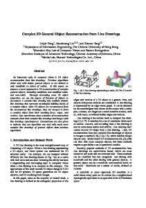
Binocular Stereo W(xw, yw,zw)
wl
(x1, y1) left image
f1
wr right image
(x2, y2)
epipolar line
f2
I
O1 centre of projection
baseline
O2 centre of projection
Figure 2.1: Binocular stereo image formation Binocular stereo or two views stereo imitates the human stereo vision and is a typical non-contact passive range sensing method. A pair of images of a 3D object (scene) are obtained from two different viewpoints under perspective projection as illustrated in figure 2.1. To obtain a 3D object from these perspective images, a distance measurement (depth) from a known reference coordinate system is computed
29
based on triangulation. The main problem in binocular stereo is to find the correspondences in stereo pair called the stereo correspondence problem. In this section, some concepts (camera model, epipolar geometry, rectification and disparity map) related to stereo correspondence problem have been introduced.
2.1.1
Correspondence Analysis
Correspondence analysis tries to solve the problem of finding which pixels or objects in one image correspond to which pixels or objects in the other. The algorithms can roughly be divided into feature based and area based, also known as region based or intensity based. Area based algorithms solve the correspondence problem for every single pixel in the image. Therefore these algorithms take color values and/or intensities into account as well as a certain pixel neighborhood. A block consisting of the middle pixel and its surrounding neighbors will then be matched to the best corresponding block in the second image. These algorithms result in dense depth values as the depth is known for each pixel. However selecting the right block size is difficult because a small neighborhood will lead to less correct maps but short run times whereas a large neighborhood leads to more exact maps at the expense of long run times. On the other hand, feature based correspondence algorithms extract the features from first image and then try to detect these features in the second image. These features should be unique within the images, like edges, corners, geometric figures, hole objects or part of objects. The resulting maps will be less detailed as the depth is
30
not calculated for every pixel. There is less possibility to match a feature incorrectly due to its detailed description, so feature based algorithms are less error sensitive and result in very exact depth values. Besides the major correspondence algorithms, area based and feature based, there are also phase based algorithms which transform the images using fast Fourier transformation (FFT). The depth is therefore proportional to the phase displacement. Wavelet based algorithms are subcategories of phase based algorithms and use wavelet transformation. There are a number of subproblems of the correspondence problem. An object seen by one of the camera could be occluded in the other camera that has a slightly different point of view. This object will cause wrong correspondences when trying to match images. The cameras itself may cause distorted images due to lens distortion which will lead to wrong correspondences especially in the outer regions of the image. Some more problems are caused by the objects themselves. Due to more number of small objects or a special pattern that repeats, quite often makes it hard to find the matching object as there are more than one possible match. This is known as the aperture problem. Another big problem is homogeneity. Large homogeneous regions are difficult to match when seen through a small window. The same textures on different positions in the image will cause similar problems. There are a number of constraints which ease the corresponding problem and improve the results like similarity, uniqueness, continuity and ordering. Another possibility to improve these
31
correspondence algorithms are some pre-processing steps like pre-reduction of noise with a low-pass filter, the adjustment of different illuminations or a white balance of each camera but the most effective pre-processing step is the calibration of the cameras and the use of epipolar constraint. These two constraints are described briefly in preceding subsections.
2.1.2
Epipolar Geometry
With two cameras arranged arbitrarily, the general epipolar geometry is shown in figure 2.2(a). The relative position of both the cameras are known as the optical centers C1 and C2 of each camera. The straight line that connects both the optical centers, is called baseline. Each point W , observed by two cameras at the same time along with the two corresponding light rays through the optical centers C1 and C2 , form an epipolar plane. The epipole e is the intersection of baseline with the image plane. The epipolar line is therefore defined as a straight line g through e and w which is intersection of the line through W and the optical center with the respective image plane. The point W in figure 2.2(b) is projected as wl in the left image plane. The corresponding point in the right image therefore lies on the previously described epipolar line g. This reduces the search space from two dimensional, which would be the whole image, to one dimensional, a straight line only. A simplification of the general epipolar geometry is shown in figure 2.4. Both cameras are arranged in parallel, their focal lengths are identical and the two retinal planes are the same. Assuming these conditions, all epipolar lines are horizontal
32
within the retinal planes and the projected images wl and wr of a point W will have
Figure 2.2: Epipolar geometry: (a) General, (b) Standard
the same vertical coordinate. Therefore the corresponding point of wl lies on the same horizontal line in the right image. According to the stereo epipolar geometry, the disparity as seen in figure 2.3(b) is defined as d = C2 − C1 . The depth Z therefore
33
is calculated by triangulation Z=b
f d
(2.1.1)
where b is the distance between the two optical centers and f is the focal length. A disparity of zero indicates that the depth of the appropriate point equals to infinity. In order to assure the stereo epipolar geometry, the rectification of both images is necessary. Therefore both cameras need to be calibrated first in order to get the camera parameters which are needed for the rectification. The next section will deal with the problem of camera calibration and image rectification.
2.1.3
The Pinhole Camera Model
Every camera maps the points of the three dimensional environment to a two dimensional image. The simplest camera model that models this mapping is the pinhole camera model. As shown in figure 2.3(a), the pinhole camera model consists of two screens. Re is the retinal plane where the two dimensional image is formed, F is the focal plane with the optical center C in the middle. Both these planes are parallel at certain distance f which is the focal length. The straight line joining the point W of the 3D world and C is called the optical axis. Via perspective projection, this point W is mapped onto the two dimensional image. Since the focal plane is parallel to the retinal plane, the points that lie on focal plane have no image on the retinal plane.
34
Figure 2.3: (a) Pinhole Camera Model, (b) Disparity
2.1.4
Camera Parameters
In order to transform a point of the 3D world into a 2D point of the image plane the knowledge of special camera parameters is necessary. There are two kinds of camera parameters. The intrinsic or internal parameters which describe the internal geometric and optical characteristics of the camera, and the extrinsic or external parameters defining the position and orientation of the camera in a world reference system.
35
Figure 2.4: Intrinsic and Extrinsic parameters of the Camera
As seen in figure 2.4, the system for modeling two or more cameras consists of three different coordinate systems, the world reference frame (xw , yw , zw ), the camera frame (xc , yc , zc ) with the optical center as origin and the image frame (X, Y). A three dimensional point, given in homogeneous world coordinates, can be converted into the camera frame, by a rotation rij and a translation tj which is expressed by the extrinsic parameters as
xc
xw
yc = Tl yw , zw zc
where
r11 r12 r13 t1
Tl = r r r t 21 22 23 2 . (2.1.2) r31 r32 r33 t3
Then this point is converted to the two dimensional image plane using the intrinsic parameters. These are in particular the focal length f , the principle point (u0 , v0 ), which is the center of the image plane, and (k0 , k1 ) the pixel size in mm or α = f / k0
36
and β = f / k1 . The transformation using the intrinsic parameters is as follows: X xc α 0 u0 Y = Ti y c , where Ti = (2.1.3) 0 β v0 Z zc 0 0 1 Since (X, Y, Z) is homogeneous, all the three variables are divided by Z in order to get the pixel coordinates X 0 and Y 0 . Points on the focal plane, where Z = 0 and zc = 0 respectively, can not be transformed to image plane coordinates because division by zero is not defined and the straight line joining this point and the optical center does not intersect with the image plane as it is parallel to the image plane. In summary, a point given in world coordinates is transformed onto a two dimensional image plane using the following equation: xw X yw Y = Ti Tl zw Z 1
(2.1.4)
knowledge of intrinsic and extrinsic parameters of the camera allows for the rectification of images and ensures the epipolar constraint. The calculation of these parameters is the aim of camera calibration and will be discussed in chapter 4.
2.1.5
Epipolar Constraints
Knowledge of intrinsic and extrinsic parameters of each camera separately is sufficient to undistort the appropriate images but it is not sufficient to assure the epipolar constraint. The epipolar constraint ensures that the epipolar lines coincide with the horizontal scan lines, and therefore corresponding points in both the images are only
37
horizontally shifted, which reduces the search space from two-dimensional to onedimensional. Given two cameras, every point W = [xw yw zw 1]T of the world reference frame can be projected to the appropriate image frame (wl and wr ) using the transformation matrix P = Ti Tl as known from section 2.1.4 as follows: wr = Pr W,
wl = Pl W
(2.1.5)
In order to rectify the images according to the epipolar constraint these projection matrices Pl and Pr have to be adapted the following special conditions: • both camera systems need to have equal focal length • both camera systems need to have the same focal plane • the optical centers need to be constant • correspondence of the vertical coordinate of each point in the left and the right images need to be same. Using these and further conditions, Pl and Pr can be calculated and the taken images can be transformed according to the epipolar constraint.
2.1.6
Rectification Process
Given a pair of stereo images, rectification determines a transformation of each image plane such that the pairs of conjugate epipolar lines become collinear and parallel to one of the image axis (usually the horizontal one). The rectified images can be
38
thought of as acquired from a new stereo rig, through rotating the original cameras. Computation of correspondence is the main advantage of rectification. This process is very simple with the use of rectification. We assume that the stereo rig is calibrated, i.e. the old perspective projection matrices (PPMs) Pol and Por are known. The idea behind the rectification is to define two new perspective matrices Pnl and Pnr , which preserve the optical centers and with the baseline contained in the focal planes. This ensures that the epipoles are at infinity and hence these epipolar lines are parallel. In addition, to have a proper rectification, it is required that the epipolar lines are horizontal and the corresponding points have the same vertical coordinates. In this section, analytical requirements and formulations are given for the rectification process. The new PPMs will have the same orientation but different positions. Positions are same as the old cameras, whereas the orientation changes because we rotate both the cameras around the optical centers in such a way that the focal plane becomes coplanar and contain the baseline. The intrinsic parameters of both the cameras will be same. The new PPMs in terms of their factorization in the intrinsic and extrinsic parameter matrices are given as
Pnl = A[R| − RC1 ],
Pnr = A[R| − RC2 ]
(2.1.6)
where C1 and C2 are the old optical centers. The rotation matrix R is same for both the PPMs, and is computed as detailed below. The intrinsic parameter matrix A is
39
also same for both PPMs . We will specify R by means of its row vectors T r 1 T R= r2 r3T
(2.1.7)
which are x, y and z axis respectively of the camera standard reference frame, expressed in world coordinates. The algorithm for detailed rectification process is explained as follows: 1. The new x axis is parallel to baseline: r1 =
(C1 −C2 ) . kC1 −C2 k
2. The new y axis is orthogonal to x axis and to k: r2 = k ∧ r1 . 3. The new z axis is orthogonal to xy plane: r3 = r1 ∧ r2 where k is an arbitrary unit vector, that fixes the position of the new y axis in the plane orthogonal to x.
2.1.7
Disparity Map
Once both the stereo images are rectified, the next step is to find the correspondence between them. For this, define similarity or difference measures between the left and right images. Typical measures for area-based are the sum of square differences (SSD), the sum of absolute differences (SAD), the normalized cross correlation (NCC), and the census. These measures of standard geometry are defined as follows. SSD(d) =
XX i
SAD(d) =
[Il (x + d + i, y + j) − Ir (x + i, y + j)]2
XX i
(2.1.8)
j
j
|Il (x + d + i, y + j) − Ir (x + i, y + j)|
(2.1.9)
40 P P C(Il , Ir ) − i j µl µr P P N CC(d) = i j σl σr
(2.1.10)
where Il and Ir represent the left and right images of stereo pair and d denotes the disparity at a point (x, y) in the right image. µl and µr represent the mean intensities in the corresponding windows of the left and right images respectively, and σl and σr are standard deviations in the windows respectively. C(Il , Ir ) is a cross correlation between the corresponding windows: C(Il , Ir ) =
XX i
Il (x + d + i, y + j)Ir (x + i, y + j)
(2.1.11)
j
The disparity d can be found by minimizing the difference measures or by maximizing the similarity measures but due to ill-posed nature of the problem one can not find the unique correspondence.
2.2
Shape from Shading
Surfaces are bright or dark for two main reasons: their albedo and the amount of light they are receiving. A model obtaining the brightness of a surface is usually called a shading model. To recover the information about 3D structure of the surface from the shading model is called shape from shading (SFS). It has been discussed in a wide variety of context since 1975. In the ideal case, the simplest shape from shading problem is formulated as: I(x) = ρIs cosφ(x)
(2.2.1)
where x denotes a point in the image, I(x) the reflected light intensity observed at x, Is the illumination intensity, ρ the constant albedo on the surface, and φ(x) the
41
angle between the light source direction and the surface normal at the 3D point on the object surface corresponding to x. A model is shown in figure 2.5 for SFS process. It is well known that φ(x) can be calculated for a given ρIs . Thus, the shape of the object surface can be reconstructed from φ(x) by combining additional constraints such as photometric stereo, smoothness assumption on the surface and so on.
Figure 2.5: A Simple Shape from Shading Process Integration of SFS and stereo has many advantages to reconstruct both the shape and the reflectance properties of surfaces. From 1990, many researchers are working on the problem of the integration of SFS and stereo.
2.3
Artificial Neural networks
Artificial neural networks (ANN) are relatively crude electronic models based on the neural structure of the brain. The brain basically learns from experience. It is natural proof that some problems that are beyond the scope of current computers are indeed solvable by human brain due to its vast network of computing elements.
42
This brain modeling also promises a less technical way to develop machine solutions. This new approach for computing also provides a more graceful degradation during system overload than its more traditional counterparts. We may offer the following definition of a neural network. An artificial neural network is a massively parallel-distributed processor made up of simple processing units called neurons, which has a natural propensity for storing experiential knowledge and making it available for use. It resembles the brain in two respects:
1. The network from its environment through a teaching/learning process acquires knowledge.
2. Inter-neuron connection strengths, known as synaptic weights are used to store the acquired knowledge.
The procedure used to perform the teaching process is called teaching algorithm or learning algorithm, the function of which is to modify the synaptic weights of the network in an orderly fashion to attain a desired design objective. A simple mathematical model of the basic processing unit of an artificial neural network is depicted in figure 2.6. Neural Networks are also referred in literature as neurocomputers, connectionist neural networks, parallel-distributed processors, etc.
43
x1 x2 x3
. . .
w2
w1
Sun Transfer
w3
Output Path
wn
Processing Element
xn Input xn
Weights
wn
Figure 2.6: A simple processing unit (Neuron).
2.3.1
Characteristics of Neural Networks
The application of neural networks possesses the following attractive properties and capabilities.
1. Nonlinearity: An artificial neural network can be linear or nonlinear. A neural network, composed of an interconnection of nonlinear neurons, is very much suitable for nonlinear modeling of various processes or systems.
2. Adaptive Learning: Neural networks have a built-in capability to adapt their synaptic weights to change in the surrounding environment. The paradigm of modification of synaptic weights is called learning. The learning can be either
44
supervised or unsupervised. Due to inherent flexibility in the architecture of neural network, the network can be designed to change its synaptic weights in real time even when operating in non-stationary environment.
3. Self-Organization: An artificial neural network can create its own organization or representation of information that receives during learning time. This property adds more robustness to neural network design operating under changing environment.
4. Real Time Operation: Artificial neural network computations may be carried out in parallel, and special hardware devices are being designed and manufactured which take advantage of this capability.
2.3.2
Functional Approximation Capabilities of Neural Networks
The following theorem by Kolmogorov [70] is the basis for approximation capabilities of neural network for continuous functions. Theorem 2.1: Any continuous real-valued functions f (x1 , x2 , ..., xn ) defined on [0, 1]n , n ≥ 2 can be represented in the form
f (x1 , x2 , ..., xn ) =
2n+1 X j=1
gj
" n X
# φij (xi )
i=1
where gj terms are properly chosen continuous functions of one variable, and φij functions are continuous monotonically increasing functions independent of f .
45
In other words, the above theorem states that one can express a continuous multivariate function on a compact set in terms of sums and compositions of a finite number of single variable functions. Cybenko [70] stated more significant features of approximation capabilities of neural networks in the following theorem. h Theorem 2.2: Let φ be any continuous sigmoid-type function e.g., φ(ξ) =
1 (1+e−ξ )
Then, given any continuous real-valued function f on [0, 1]n (or any other compact subset of 0, there exist vectors w1 , w2 , ..., wN , α, and θ and a parameterized function G( · , w, α, θ) : [0, 1]n → < such that | G(x, w, α, θ − f (x) | < ε for all x ∈ [0, 1]n where
G(x, w, α, θ) =
N X
αj φ(wjT x + θj )
j=1
and wj ∈
2.3.3
Feed-Forward Neural Networks
A two-layer feed-forward neural network (FFNN) with n input units, m output units and N units in the hidden layer, is shown in the figure 2.7. The output vector y is determined in terms of the input vector x by the formula yi =
N X j=1
" wij σ
Ã
n X k=1
! vjk xk + θvj
# + θwi
; i = 1, · · · , m
(2.3.1)
i .
46
θ v1
V
T
σ (.)
1
WT
θ w1
x1
y1 2 σ (.)
x2
• •
xn
• •
•
•
θ wm
• • θ vN
•
ym N
σ (.)
OUTPUTS
INPUTS HIDDEN LAYER Figure 2.7: Model of a feed-forward neural network.
where σ(.) are the activation functions of the neurons of the hidden-layer. The inputs to hidden layer interconnection weights are denoted by vjk and the hidden-layer-tooutputs interconnection weights by wij . The bias weights are denoted by θvj and θwi . There are many classes of activation functions e.g. sigmoid, hyperbolic tangent and Gaussian. The sigmoid activation function used in our work, is given by
σ(x) =
1 1 + e−x
(2.3.2)
47
By collecting all the NN weights vjk and wij into matrices of weights V T and W T , we can write the ANN equation in terms of vectors as
y = W T σ(V T x)
(2.3.3)
with the vector of activation functions defined by σ(z) = [σ(z1 ) · · · σ(zn )]T for a vector z ∈
2.3.4
Function Approximation Property
Let f (x) be a smooth function from
f (x) = W T σ(V T x) + ε
(2.3.4)
The value of ε is called the NN functional approximation error. In fact, for any choice of a positive number εN , one can find a FFNN such that ε < εN in Ux . Then an estimate of f (x) can be given by ˆ T σ(Vˆ T x) fˆ(x) = W
(2.3.5)
ˆ and Vˆ are estimates of the ideal NN weights that are provided by some where W on-line weight tuning algorithms.
48
2.3.5
Error Backpropagation Algorithm
This is a common weight-tuning algorithm based on gradient descent algorithm. If the NN is training off-line to match specified exemplar pairs (xd , yd ), with xd , the ideal NN input that yields the desired NN output yd , then the continuous-time version of the backpropagation algorithm for the two-layer NN is given by ˆ˙ = F σ(Vˆ T xd )E T W ˙ ˆ E)T Vˆ = Gxd (σ T W
(2.3.6)
where F and G are positive definite design learning parameter matrices. The backpropagated error E is selected as the desired NN output minus the actual NN output, i.e., E = yd − y. For the scalar sigmoid activation function (2.3.2) the hidden-layer output gradient σ ˆ 0 is given by σ ˆ 0 ≡ diag{σ(Vˆ T xd )}[I − diag{σ(Vˆ T xd )}]
(2.3.7)
where I denotes the identity matrix, and diag[z] means a diagonal matrix whose diagonal elements are the components of the vector z.
2.3.6
Gradient Descent
Consider the optimization problem of a real-valued multidimensional scalar function (objective function) of the form y : Σ → <, where the search space Σ is a compact subset
49
y may also admit local minimum. A point x∗ is a local minimum of y if y(x∗ ) < y(x) for all x such that kx∗ − xk ≤ ε, for some ε > 0. Gradient descent is a search strategy to determine the minimum of functions that may be local or global as well. Assuming y is differentiable, gradient descent can be expressed according to the recursive rule: x(k + 1) = x(k) − ρ ∇y(x)|x(k)
k = 1, 2, · · · m, m + 1, · · ·
(2.3.8)
where ρ is a small positive constant and k is a positive integer represents iteration number. ∇y(x) denotes the gradient of y(x) and is defined as iT h ∂y ∂y ∂y . ∇y(x) = ∂x · · · ∂x2 ∂xn 1
2.4
Genetic Algorithm
Genetic algorithm (GA) was introduced by John Holland in 1975, based on a method for studying natural adaptive systems and designing artificial adaptive systems, with roots in Darwinian natural selection and Mendelian genetics. GAs search a problem representation space of artificial adaptive systems, eliminating weak elements by favoring retention of optimal and near optimal individuals (survival of the fittest), and recombining features of good individuals to perhaps make better individuals. The elements of search space represent the possible solutions to the problem and are coded as strings (chromosomes), derived from an alphabet. They work with coding of the problem rather than the problem itself. Such characteristic has made them to be known as robust optimization methods. In order to use a GA approach, it is necessary to first derive an initial population of chromosomes (potential solutions) and set a cost
50
function to measure each chromosomes fitness. The best solution is then searched in the solution space. The optimization is performed by manipulating the population of chromosomes, during a number of generations, in each of which the GA creates a set of new individual by crossover and mutation operations, similar to natural reproduction processes. The crossover operation takes two parent chromosomes and mates them to produce two child chromosomes. The mutation operation is used for exploring new regions in the search space, thus maintaining population diversity. GAs are particularly suitable for applications that require adaptive problem-solving strategies. A GA typically consists of the following components: • A population of strings or coded possible solutions (chromosomes) • A mechanism to encode a possible solution (binary or real) • Objective function and associated fitness evaluation techniques • Selection/reproduction procedure • Genetic operators (crossover and mutation) • Probabilities to perform genetic operations Let us briefly describe these components: Population– To solve an optimization problem, GAs start with the chromosome (structural) representation of a parameter set (x1 , x2 , ..., xp ). The parameter set is
51
to be coded as a finite length string over an alphabet of finite length. The coding is binary or real. In binary coded GA, the chromosomes are strings of 0’s and 1’s. Each chromosome actually refers to a coded possible solution. A set of such chromosomes in a generation is called a population. The size of a population may vary from one generation to another or it may be constant. Usually, the initial population is chosen randomly. Encoding/decoding mechanism– It is the mechanism to convert the parameter values into chromosome representation. Decoding is just the reverse of encoding. Objective function– The objective/ fitness function is chosen depending on the problem. It is chosen in such a way that highly fitted strings (possible solutions) have high fitness values. It is only index to select a chromosome to reproduce for the next generation. Selection/ reproduction procedure– The selection/reproduction procedure copies individual strings into a tentative new population for genetic operations. The number of copies reproduced for the next generation by an individual is expected to be directly proportional to its fitness value. Roulette wheel parent selection, tournament selection and linear selection are some famous selection procedures. Crossover– The main purpose of crossover is to exchange information between randomly selected parent chromosomes with the aim of not losing any important information. Actually, it recombines genetic material of two parent chromosomes to produce offspring for the next generation. Some of the commonly used crossover techniques are
52
one-point crossover, two-point crossover, multiple-point crossover, uniform crossover and so on. A newly developed crossover technique namely Laplacian crossover has been used in our work. Mutation– Mutation generates the diversity into the population. Sometimes, it helps to regain the information lost in earlier generations. Mutation in GA perform occasionally. Probabilities to perform genetic operations– The probability to perform crossover operation is chosen in a way so that the recombination of potential strings increase without any disruption. The probability to perform mutation is very low because it occurs occasionally. Crossover and mutation probabilities may be kept fixed throughout the operation of a GA or they may also be made adaptive to improve the performance. A schematic diagram of the basic structure of a GA is shown in figure 2.8.
2.4.1
Distinguishing Characteristics
The following features facilitate GA to enhance their applicability over the most commonly used optimization and searching strategies:
• GAs work simultaneously on multiple points and not a single point. This feature prevents it from getting stuck at local optimal, to some extent.
• GAs work with the coded parameter set, not with the parameters themselves. Hence, the resolution of possible search space can be controlled by varying the
53
# "
!
$
Figure 2.8: Flow Chart for Genetic Algorithm coding length of the parameters. • The search space need not be continuous. • GAs use probabilistic transition rules, not deterministic ones. Recently, GAs are used to solve the various problems in computer vision like camera calibration, correspondence problem etc. In the next chapter, a methodology to reconstruct various algebraic curves in 3D space from corresponding arbitrary perspective views is presented.
54
Chapter 3 RECONSTRUCTION OF ALGEBRAIC CURVES IN 3D SPACE FROM 2D ARBITRARY PERSPECTIVE VIEWS 3.1
Introduction
This chapter is concerned with the reconstruction of algebraic curves in 3D space from arbitrary perspective views. The advantages of proposed method is to overcome the matching problem that occurs in pair of projections of the curve and reconstruction of algebraic curves which do not lie on a plane (non-planar curve). Parameters of a curve in 2D digitized image planes are determined using least-square curve fitting. From this, conical surfaces are obtained which are spanned by the curves and the center of focus of the respective cameras. Equations for reconstruction of the 3D curve, which give their parameters are determined. Uniqueness of the solution in the process of reconstruction is addressed and solved using additional constraints. As practical examples, reconstruction of circles, parabolic curves, pair of straight lines 55
56
and cubic curves in 3D space are demonstrated. Some results are also presented in the case of real images. Most of the natural as well as man-made objects have curved lines and surfaces. Reconstruction of curved lines of 3D objects is an important task in many applications of computer vision such as estimation of 3D object structure, object recognition and reconstruction. For objects with planar shapes, straight lines and points are used as features for reconstruction. This is not useful for objects with curved surfaces. For objects with curved surfaces, the intersection of two surfaces (3D edge) is a curve. The case of reconstruction of algebraic curves in 3D space has been discussed by several authors in their work, Xie et al. [176, 177], Rothwell et al. [141], Kanantani et al. [88, 89, 90], Ma [102], Quan [133], M-H An et al. [4], Kahl et al. [84], Balasubramanian et al. [13], Shukla et al. [153]. Though Xie et al. [176] give the analytical formulation for the reconstruction of quadratic curves, they have not given any methodology to determine the unique solution from the roots of a quadratic equation. In the case of planar curves, they have assumed the existence of a point to point correspondence between the sets of contour points on the pair of projected curve segments. Kanatani et al. [88] have developed computation procedures to interpret the 3D geometry of conics in the scene from their projections by giving real examples. Ma [102] have proposed a method to obtain the closed form solution of correspondence problem and for global reconstruction of conics in 3D space. Xie [177] uses the planarity constraint and formulations given in Xie et al. [176] to obtain the
57
unique solution in case of conics using point to point correspondence and has described a method to improve the quality of 3D data related to conics. Quan [133] has solved correspondence in the case of conics from two views. He has solved the ambiguity (non-uniqueness) in the solutions with the use of a non-transparency constraint of a conic section. M-H An et al. [4] have proposed a methodology for the reconstruction of the plane on which the conic in 3D space lies. Projection of these curves onto image planes under perspective transformation produce conics. Two or more corresponding conics, from as many views, are used to reconstruct a curve in 3D. Balasubramanian et al. [13] have proposed a method to reconstruct the quadratic curves in 3D space with the help of intersection of a line and a cone. Shukla et al. [153] have proposed a methodology for the reconstruction of a parabola in 3D space together with the error analysis in reconstruction process. The work presented in this chapter deals with the methodology of reconstruction of an algebraic curve in 3D space from two or more arbitrary perspective views. Equations of reconstruction are presented, along with the examples from simulation studies. The issue of uniqueness of the solution is addressed and solved with the use of additional constraints. Error analysis has been discussed in reconstruction process on the basis of different criterion. Rest of the chapter is organized as follows. Section 3.2 contains the model of imaging setup. The reconstruction methodology has been described in section 3.3. Section 3.4 contains the application of proposed methodology in case of quadratic
58
curves. The applications of proposed methodology in cubic curves are presented in section 3.5. Reconstruction results for real images are shown in section 3.6.
3.2
Imaging Setup
The imaging set-up using two cameras is shown in Figure 3.1. Let I1 and I2 be the first and second image planes of the pair of cameras C1 and C2 respectively. Let the position and the orientation of one camera be known with respect to another and both have a common field of view. Let O1 xyz be the rectangular cartesian frame of reference with its origin O1 at the center of projection of one of the cameras C1 . A point W in 3D space, with co-ordinates (Xw , Yw , Zw ) with respect to the frame of reference at C1 , is viewed by both the cameras C1 and C2 . Let O2 x0 y 0 z 0 be the second rectangular cartesian co-ordinate system, not necessarily parallel to O1 xyz system, with its origin O2 at the center of projection of the second camera C2 . Let the coordinates of the second camera C2 with respect to O1 be (xd , yd , zd ). Let P1 (X1 , Y1 , f1 ) and P2 (X2 , Y2 , f2 ) be the corresponding pair of projections of point W on the pair of image planes I1 and I2 respectively. Let f1 and f2 be the focal lengths of the first and the second cameras respectively. Let the perspective projections of an algebraic curve Γ in 3D space be a pair of algebraic curves Γ1 and Γ2 , on the first and second image planes respectively as shown in Figure 3.1. The problem is to reconstruct the 3D algebraic curve Γ from a pair of its images Γ1 and Γ2 . The relation between the coordinates of the point W (xw , yw , zw ) and that of the image point P (X1 , Y1 , f1 ) is
59
given by the perspective equation: X1 = f1
xw , zw
Y 1 = f1
yw zw
(3.2.1)
The 3D co-ordinates of point W(xw , yw , zw ) with respect to second camera C2 , is given by
x0
cos α1 cos β1 cos γ1
(xw − xd )
y 0 = λ cos α2 cos β2 cos γ2 (yw − yd ) 0 z cos α3 cos β3 cos γ3 (zw − zd )
(3.2.2)
In the above equations αi , βi , γi (i = 1, 2, 3) are the respective direction cosines of the axes of O2 x0 y 0 z 0 with respect to O1 xyz system and can be expressed in θ, φ and ψ (Eulerian angles). λ is a scale factor between the two reference frames and without loss of generality this is considered to be 1, in the present work. Using equation (3.2.2), the relation between the object space point W (xw , yw , zw ) and the image point P2 (X2 , Y2 , f2 ) is given as follows: (xw − xd )cosα1 + (yw − yd )cosβ1 + (zw − zd )cosγ1 (xw − xd )cosα3 + (yw − yd )cosβ3 + (zw − zd )cosγ3 (xw − xd )cosα2 + (yw − yd )cosβ2 + (zw − zd )cosγ2 Y2 = f2 (xw − xd )cosα3 + (yw − yd )cosβ3 + (zw − zd )cosγ3
X2 = f2
(3.2.3) (3.2.4)
Equations (3.2.1), (3.2.3) and (3.2.4) are the collinearity equations for a pair of arbitrary perspective views.
3.3
Reconstruction Methodology
In this work, least-square curve fitting has been used to obtain the parameters of the projected algebraic curves in various 2D image planes. A fully calibrated imaging
60
Ƚ S2
W (Xw, Yw, Zw)
I2 S1
z’ X2
I1 f2
z
x’ f1 Ƚ2
P2 (X2, Y2, Z2)
O2 (Xd, Yd, Zd)
Y1
Ƚ1 X1
y
Y2
P1 (X1, Y1, Z1) O1 (0, 0, 0) x
Figure 3.1: Model for Imaging Setup
y’
61
setup has been used for the reconstruction of algebraic curve in 3D space. The knowledge of following input parameters is necessary for the reconstruction process. • The set of pixel coordinates for the curve Γ1 on the first image plane I1 : (X1i , Y1i ), i = 1, 2, ....., m. • The set of pixel coordinates for the curve Γ2 on the second image plane I2 : (X2i , Y2i ), i = 1, 2, ....., n. • The set of pixel coordinates for the curve Γ3 (additional constraint for uniqueness) on the third image plane I3 : (X3i , Y3i ), i = 1, 2, ....., p. • Intrinsic and extrinsic parameters for all cameras i.e. focal lengths, center of focus etc. We assume that f1 = f2 = 1 for the computational simplicity. Let the equations of the conics Γ1 and Γ2 in the respective first and second image planes I1 and I2 which obtained from least-square curve fitting is represented by the polynomials Γ1 :
X
aijk X1i Y1j = 0
(3.3.1)
bijk X2i Y2j = 0
(3.3.2)
i+j+k=n
Γ2 :
X
i+j+k=n
Substituting the collinearity equations given by equations (3.2.1),(3.2.3) and (3.2.4) in the equations (3.3.1) and (3.3.2), we obtain the representation of conical surfaces S1 and S2 (assume f1 = f2 = 1): S1 :
X i+j+k=n
aijk xiw ywj zwk = 0
(3.3.3)
62
S2 :
X
i
j
k
bijk x0 w y 0 w z 0 w = 0
(3.3.4)
i+j+k=n
By transforming (x0 , y 0 , z 0 ) in equation (3.3.4) to (x, y, z) using the camera extrinsic parameter data (see equation (3.2.2)), S2 can be represented using the same coordinate system as S1 : S2 :
X
b0ijk xiw ywj zwk = 0
(3.3.5)
i+j+k≤n
Notice that the equations (3.3.3) and (3.3.4) are homogenous polynomials of degree n, while equation (3.3.5) is non homogeneous polynomial of degree n, because origin of the coordinate system O1 is not located on the surface S2 . It is clear from the model of imaging setup explained in section 3.2 that the required curve Γ in 3D space is the intersection of two surfaces represented by S1 and S2 . The intersection of these two conic surfaces may have some extra points other than the required curve Γ. To avoid these extra points, the third perspective view Γ3 of Γ has been used. All points obtained from the intersection of S1 and S2 have been projected on the third image plane and from these points the required curve in 3D space has been obtained. The following steps have been performed for the reconstruction and uniqueness of algebraic curve Γ in 3D space. • Calculate S12 and S22 . • Construct a function F which is defined as F (x, y, z) = S12 (x, y, z) + S12 (x, y, z). • Minimize the function F using suitable unconstrained optimization technique.
63
Here nonlinear least square technique has been used to optimize the function F. • Find the sets of values (x, y, z) for which the function F is zero or very close to zero. • Project all these points in the third view I3 . • Select the points which coincide with Γ3 in the image plane I3 . These are the points of reconstructed curve Γ in 3D space.
3.4 3.4.1
Case of Quadratic Curves Mathematical Formulation
In this section, the detailed process has been explained in the case of quadratic curve Γ, where n = 2 in the equations starting from (3.3.1) to (3.3.5). Let the equation of the curve Γ1 in the first image plane I1 be 2 2 Av1 Xv1 + Bv1 Yv1 + Cv1 Xv1 Yv1 + Dv1 Xv1 + Ev1 Yv1 + Fv1 = 0
(3.4.1)
Let (X1 , Y1 ) be a point on the curve Γ1 , using(3.2.1) and (3.4.1) results in, Av1 {f1
xw 2 yw xw yw xw xw } + Bv1 {f1 }2 + Cv1 {f1 }{f1 } + Dv1 {f1 } + Ev1 {f1 } + Fv1 = 0 zw zw zw zw zw zw (3.4.2)
Av1 f12 x2w + Bv1 f12 yw2 + Cv1 f12 xw yw + Dv1 f1 xw zw + Ev1 f1 yw zw + Fv1 zw2 = 0
(3.4.3)
Equation (3.4.3) is the equation of a surface passing through the origin. Normalizing
64
the above equation, the equation of the surface S1 reduces to, A1n x2w + B1n yw2 + C1n xw yw + D1n xw zw + E1n yw zw + zw2 = 0
(3.4.4)
where A1n = {
Av1 f12 }, B1n Fv1
={
Bv1 f12 }, C1n Fv1
={
Cv1 f12 }, D1n Fv1
= { DFv1v1f1 }, E1n = { EFv1v1f1 }
The surface denoted by equation (3.4.4) is a cone in 3D having vertex as origin. Let us denote this by S1 (xw , yw , zw ). Now the equation of the curve Γ2 on the second image plane I2 be, 2 2 Av2 Xv2 + Bv2 Yv2 + Cv2 Xv2 Yv2 + Dv2 Xv2 + Ev2 Yv2 + Fv2 = 0
(3.4.5)
Since (X2 , Y2 ) is a point on the curve Γ2 , using the collinearity equations again, the above equation (3.4.5) reduces to (assume f2 = 1) Av2 {
x0w 2 yw0 2 x0w yw0 x0w x0w } + B { } + C { }{ } + D { } + E { } + Fv2 = 0 v2 v2 v2 v2 zw0 zw0 zw0 zw0 zw0 zw0
(3.4.6)
or the above equation can be written as 02 0 0 0 0 0 0 02 Av2 x02 w + Bv2 yw + Cv2 xw yw + Dv2 xw zw + Ev2 yw zw + Fv2 zw = 0
(3.4.7)
where (x0w , yw0 , zw0 ) is the object point W in 3D space with respect to the second camera system O2 (xd , yd , zd ). With respect to O1 (0, 0, 0) the above equation can be written as
Av2 [(xw − xd )cosα1 + (yw − yd )cosβ1 + (zw − zd )cosγ1 ]2 + Bv2 [(xw − xd )cosα2 + (yw − yd )cosβ2 + (zw − zd )cosγ2 ]2 +Cv2 [(xw −xd )cosα1 +(yw −yd )cosβ1 +(zw −zd )cosγ1 ][(xw −xd )cosα2 +(yw −yd )cosβ2 +
65
(zw − zd )cosγ2 ] +Ev2 [(xw −xd )cosα1 +(yw −yd )cosβ1 +(zw −zd )cosγ1 ][(xw −xd )cosα3 +(yw −yd )cosβ3 + (zw − zd )cosγ3 ] +Fv2 [(xw −xd )cosα2 +(yw −yd )cosβ2 +(zw −zd )cosγ2 ][(xw −xd )cosα3 +(yw −yd )cosβ3 + (zw − zd )cosγ3 ] + Gv2 [(xw − xd )cosα3 + (yw − yd )cosβ3 + (zw − zd )cosγ3 ]2 = 0
Let xd cosαk + yd cosβk + zd cosγk = Aαk for k=1,2 and 3, then the above equation becomes,
A1 x2w + A2 yw2 + A3 zw2 + A4 xw yw + A5 yw zw + A6 zw xw + A7 xw + A8 yw + A9 zw + A10 = 0 (3.4.8) which represents the equation of the surface S2 , where A1 = Av2 cos2 α1 + Bv2 cos2 α2 + Cv2 cosα1 cosα2 + Dv2 cosα1 cosα3 + Ev2 cosα2 cosα3 + Gv2 cos2 α3 A2 = Av2 cos2 β1 + Bv2 cos2 β2 + Cv2 cosβ1 cosβ2 + Dv2 cosβ1 cosβ3 + Ev2 cosβ2 cosβ3 + Gv2 cos2 β3 A3 = Av2 cos2 γ1 + Bv2 cos2 γ2 + Cv2 cosγ1 cosγ2 + Dv2 cosγ1 cosγ3 + Ev2 cosγ2 cosγ3 + Gv2 cos2 γ3 A4 = 2Av2 cosα1 cosβ1 + 2Bv2 cosα2 cosβ2 + Cv2 (cosα1 cosβ2 + cosα2 cosβ1 ) +Ev2 (cosα1 cosβ3 +cosα3 cosβ1 )+Fv2 (cosα2 cosβ3 +cosα3 cosβ2 )+2Gv2 cosα3 cosβ3
66
A5 = 2Av2 cosγ1 cosβ1 + 2Bv2 cosγ2 cosβ2 + Cv2 (cosγ1 cosβ2 + cosγ2 cosβ1 ) + Ev2 (cosγ1 cosβ3 + cosγ3 cosβ1 ) + Fv2 (cosγ2 cosβ3 + cosγ3 cosβ2 ) + 2Gv2 cosγ3 cosβ3 A6 = 2Av2 cosγ1 cosα1 + 2Bv2 cosγ2 cosα2 + Cv2 (cosγ1 cosα2 + cosγ2 cosα1 ) + Ev2 (cosγ1 cosα3 + cosγ3 cosα1 ) + Fv2 (cosγ2 cosα3 + cosγ3 cosα2 ) + 2Gv2 cosγ3 cosα3 A7 = −{2Av2 Aα1 cosα1 + 2Bv2 Aα2 cosα2 + Cv2 (cosα1 Aα2 + cosα2 Aα1 ) + Ev2 (cosα1 Aα3 + cosα3 Aα1 ) + Fv2 (cosα2 Aα3 + cosα3 Aα2 ) + 2Gv2 Aα3 cosα3 A8 = −{2Av2 Aα1 cosβ1 + 2Bv2 Aα2 cosβ2 + Cv2 (cosβ1 Aα2 + cosβ2 Aβ1 ) + Ev2 (cosβ1 Aα3 + cosβ3 Aα1 ) + Fv2 (cosβ2 Aα3 + cosβ3 Aα2 ) + 2Gv2 Aα3 cosβ3 A9 = −{2Av2 Aα1 cosγ1 + 2Bv2 Aα2 cosγ2 + Cv2 (cosγ1 Aα2 + cosγ2 Aα1 ) + Ev2 (cosγ1 Aα3 + cosγ3 Aα1 ) + Fv2 (cosγ2 Aα3 + cosγ3 Aα2 ) + 2Gv2 Aα3 cosγ3 A10 = Av2 A2α1 + Bv2 A2α2 + Cv2 Aα1 Aα2 + Ev2 Aα1 Aα3 + Fv2 Aα2 Aα3 + Gv2 A2α3 The surface denoted by Equation (3.4.8) is a cone in 3D space having vertex on O2 (xd , yd , zd ) and denoted by S2 (xw , yw , zw ). Intersection of surfaces represent by equations (3.4.4) and (3.4.8) gives the point of reconstructed curve Γ. Define a function F as follows: F (xw , yw , zw ) = S12 (xw , yw , zw ) + S22 (xw , yw , zw )
(3.4.9)
The function F has been minimized using nonlinear least square optimization technique with some suitable initial roots and obtain the 3D set of points (xw , yw , zw ) which satisfy both the equations (3.4.4) and (3.4.8). These are the reconstructed points of quadratic curve Γ in 3D space using two images Γ1 and Γ2 . The reconstructed points need not represent a conic because intersection of two surfaces (cones)
67
may be a surface again, but it contains the required conic. These extra points are omitted with the help of third perspective view of required curve Γ.
3.4.2
Reconstruction Results
The methodology discussed in the above section have been implemented for the quadratic curves such as circles, parabolic curves, ellipses and pair of straight lines to obtain the sequence of points in which some of them lie on the curve or the neighborhood of the curve. In order to remove the points that do not lie on the curve, the additional constraint called the third perspective view is considered. This consists of the projection of the original curve Γ, i.e., a set of pixel coordinates for the corresponding curve, Γ3 : (X3i , Y3i ), i = 1, 2, ....., n. Again, the least square curve fitting has been used to construct a curve (in third view) and let the equation of this curve be f3 (X, Y ) = 0. Now project the reconstructed 3D points (obtained from the intersection of S1 and S2 ) on this image plane and select the points whose projection in the third view, (X, Y ), that satisfies the equation f3 (X, Y ) = 0. For computational purpose some suitable threshold values (²) are considered. Figures 3.2 and 3.3 represent the reconstruction of parabola in 3D space and the projection of the original and the reconstructed points in the third view and in the case of prefect stereo with the various amount of noise. The thicker solid line represents the original curve and the dotted line or starred line represents the reconstructed points that satisfies the equation f3 (X, Y ) = 0, with the suitable threshold values ². The equation of the curve and values for the various parameters of the imaging setup
68
are given in the caption. Figures 3.4 and 3.5 represent the reconstruction of an ellipse in 3D space and the projection of the original and the reconstructed points in third view and in the case of perfect stereo with various amount of noise. In the noise free cases, the reconstructed curve that obtained from the proposed methodology coincide with the original curves. Figures 3.6 and 3.7 represent the reconstruction of the pair of straight lines in 3D space and the projection of the original and the reconstructed points in the third view and in the case of perfect stereo with various amount of noise. It can be seen that the reconstruction process in case of little amount of noise gives better result and do not affect our methodology very much. From the above figures, it is observed that our algorithm works very well for the noise free cases as well as small amount of noise. Figures 3.8 and 3.9 represent the reconstruction of parabola in 3D space and the projection of the original and the reconstructed points in the third view and in the general case with various amount of noise.
69
41 ____ : Original
zw
40.5
+++ : Reconstructed
40
39.5
39 20 300
10 250 200
0
150 100
−10
50 −20
y
0 −50
x
w
w
1
____ +++
***
<> <>
Original Reconstructed Reconstructed (Variace= 1.0) Reconstructed (Variance= 5.0)
0.5
0
−0.5 −2
0
2
4
6
8
10
Figure 3.2: Reconstruction of a parabola in 3D (top) in the case of perfect stereo and in the absence of noise. Projection of the original and reconstructed points in the third view (bottom). Equation of the parabola is considered as xw (t) = 16t2 , yw (t) = 4t and zw (t) = 40. In this case the parameters are f1 = f2 = 1, xd = 100, yd = 0.0, zd = 0.0.
70
41
zw
40.5
40
39.5
39 20
___ : Original curve +++: Reconstructed curve
10
400 300
0
200 100
−10 0 −20
yw
−100
xw
41
zw
40.5
40
39.5
39 40
___ : Original curve 30
+++: Reconstructed curve
300
20
250 10
200 150
0
100
−10 yw
50 −20
0
xw
Figure 3.3: Reconstruction of a parabola in 3D in the case of perfect stereo and in the presence of Gaussian noise of variance 1.0 (top) and variance 5.0 (bottom). Equation of the parabola is considered as in figure 3.2.
71
0.8
___ Original
0.7
+++ Reconstructed
zw
0.6 0.5 0.4 0.3 8
10 6 5
4 2
yw
0 0 −2
xw
−5
25
20
:original +++++ :reconstructed <><><> :reconstructed (vaiance=0 .1) :reconstructed (vaiance=5.0)
15
Y
******
10
5
0
−5 −10
−5
0
5
10
15
20
25
X
Figure 3.4: Reconstruction of an ellipse in 3D (top) in the case of perfect stereo and in the absence of noise. Projection of the original and reconstructed points in the third view (bottom). Equation of the ellipse is considered as xw (t) = 5 + 3cos(t) − 2sin(t), yw (t) = 4 − 2cos(t) + 3sin(t) and zw (t) = .82 − .02cos(t) − .02sin(t). In this case the parameters are f1 = f2 = 1, xd = 15, yd = 0.0, zd = 0.0.
72
___ Original 0.7
+++ Reconstructed
zw
0.6
0.5
0.4
0.3 8 8
6 6
4
4 2
2 0
0
−2 −2
yw
−4
xw
___ Original +++ Reconstructed
0.45
zw
0.4 0.35 0.3 0.25 8
8 6
6 4 4 2
yw
2
0 0
−2 −2
xw
−4
Figure 3.5: Reconstruction of an ellipse in 3D in the case of perfect stereo and in the presence of Gaussian noise of variance 1.0 (top) and variance 5.0 (bottom). Equation of the ellipse is considered as in figure 4.
73
11 ___: Original curve 10.5
***: Reconstructed curve
zw
10
9.5
9 12 10
9 8
8
7 6
6
5 4
y
4
xw
w
1.2 ____ 1.1
**** <> <> +++
Original curve Reconstructed curve Reconstructed (variance 0.0001) Reconstructed (variance = 1.0)
1
Y
0.9
0.8
0.7
0.6
0.5
0.4 0.3
0.4
0.5
0.6
0.7
0.8
0.9
X
Figure 3.6: Reconstruction of a pair of straight lines in 3D (top) in the case of perfect stereo and in the absence of noise. Projection of the original and reconstructed points in the third view (bottom). Equation of the pair of straight lines is considered as xw (t) = 4 + 5t, yw (t) = 5 + t and zw (t) = 10, xw (t) = 4 + 4t1 , yw (t) = 5 + 5t1 and zw (t) = 10. In this case the parameters are f1 = f2 = 1,0 ≤ t ≤ 1, xd = 20, yd = 0.0, zd = 0.0.
74
11 ___: Original
zw
10.5
+++: Reconstructed
10
9.5
9 10 9
9 8
8 7
7 6
6
5 5
y
4
x
w
w
11 10.5 10 9.5
___: Original curve ***: Reconstructed curve
9 10
9 8
9 7
8 6
7 5
6 5
4
Figure 3.7: Reconstruction of a pair of straight lines in 3D in the case of perfect stereo and in the presence of Gaussian noise of variance 1.0 (top) and variance 5.0 (bottom). Equation of the pair of straight lines is considered as in figure 3.6.
75
115 ___: Original 110
*** : Reconstructed
zw
105
100
95
90 160 140
80 120
60 40
100 20
80
0 60
yw
−20
x
w
1.6 +++ 1.5
1.4
1.3
Y
1.2
1.1
1
0.9
0.8
0.7
:original :reconstructed :reconstructed (vaiance=0 .2) :reconstructed (vaiance=1.0)
**** +++ <><><
−0.1
0
0.1
0.2
0.3
0.4
0.5
0.6
0.7
0.8
0.9
X
Figure 3.8: Reconstruction of a parabola in 3D (top) in general case and in the absence of noise. Projection of the original and reconstructed points in the third view (bottom). Equation of the parabola is considered as xw (t) = 40+9.96195t−0.31751t2 , yw (t) = 70 + .59696t + 4.980975t2 and zw (t) = 100 + .63502t + .29848t2 , In this case the parameters are f1 = f2 = 1,−4 ≤ t ≤ 4, xd = 30, yd = 80, zd = 30, θ = π4 , φ = π4 , ψ = π4 .
76
120 ___ : Original 115 **** : Reconstructed
zw
110 105 100 95 90 160 140
80 120
60 40
100 20
80
0 60
yw
−20
x
w
120 110 100
zw
90 80
____
70
***
Original Reconstructed
60 50 40 160 140
100 80
120 60
100
40 20
80 yw
0 60
−20
xw
Figure 3.9: Reconstruction of a parabola in 3D in the general case and in the presence of Gaussian noise of variance 0.2 (top) and variance 1.0 (bottom). Equation of the pair of parabola is considered as in figure 3.8.
77
3.4.3
Error Analysis
The criterion used for computing the error in reconstruction is the angle between the planes in which the original and the reconstructed quadratic curves lie. Noise with Gaussian distribution is added to the pixel coordinate values of the projection of a quadratic curve on the image plane. This perturbs the location of pixel forming the projection of the quadratic curve on the image plane, simulating the effect of noise. The level of noise is characterized by the variance, σ of the Gaussian distribution. Let the equation of the planes in which the original and the reconstructed curve lies be Ai x + Bi y + Ci z + Di = 0,
for i = 1, 2
(3.4.10)
Therefore cosine of the angle between the two planes is given by
cos(δ) = p
A1 A2 + B1 B2 + C1 C2 p A21 + B12 + C22 A22 + B22 + C22
(3.4.11)
δ is the error in the reconstruction. Using simulation studies, the error is estimated for different combinations of the geometry of the imaging setup, parameters of the quadratic curves and the level of noise added to the image planes. Each of the plots in figure 3.10, illustrate that errors vary nonlinearly with respect to different combinations of the parameters which described above. The plots are drawn between variance vs angle in degrees. In a perfect stereo case, as shown in top and middle plot of figure 3.10, starting σ=0.0 to 4.0, it is observed that there is almost very little error. This suggests that
78
our algorithm works very well even in the noisy cases in the case of perfect stereo. However, for σ ≥ 5.0(higher noisy cases) the error is gradually increasing. In general case, as shown in figure 3.10 (bottom), as σ increases the error also gradually increases. From σ=0.0 to 0.3 it is observed that there is no error and these cases are equivalent to noise free. When σ ≥ 0.4, one can see the gradual increment in the error. 20
25
18
16
20
Errors in Degrees
Error in Degrees
14
12
10
8
15
10
6
4
5
2
0
0
1
2
3 Variance
4
5
0
6
0
1
2
3 Variance
4
5
6
25
Errors in degrees
20
15
10
5
0 −0.1
0
0.1
0.2
0.3
0.4
0.5
0.6
Variance
Figure 3.10: Error analysis in reconstruction of parabola in prefect stereo (top), ellipse in prefect stereo(midle) and parabola in general case. Equation of the parabola is considered as xw (t) = 16t2 , yw (t) = 4t and zw (t) = 40. In this case the parameters are f1 = f2 = 1, xd = 100, yd = 0.0, zd = 0.0.
79
3.5
Case of Cubic Curves
3.5.1
Mathematical Formulations
In the previous section, the proposed methodology has been applied for the reconstruction of various quadratic curves. In this section, this methodology is implemented in the reconstruction of cubic curves. Here, the meaning of cubic curve is the curve that represents by a third degree polynomial (i.e. n=3). In case of cubic curves, the equation of surface S1 (see section 3.3) can be written as
A1n x3w + B1n yw3 + C1n x2w yw + D1n xw yw2 + E1n xw yw zw
(3.5.1)
+F1n x2w zw + G1n yw2 zw + H1n xw zw2 + I1n yw zw2 + J1n zw3 = 0
and equation of the surface S2 is given as
A1 x3w + A2 yw3 + A3 zw3 + A4 xw yw zw + A5 x2w yw + A6 xw yw2 + A7 x2w zw +
(3.5.2)
A8 yw2 zw + A9 xw zw2 + A10 yw zw2 + A11 x2w + A12 yw2 + A13 zw2 + A14 xw yw + A1 5yw zw + A16 xw zw + A17 xw + A18 yw + A19 zw + A20 = 0
where Ai ’s, i = 1(1)20 are functions of rotational and translation parameters of second camera. These parameters are given by very big expression and can be obtained by using similar method as given in the case of quadratic curve. The required cubic curve Γ is obtained by projecting the intersection points of equations (3.5.1) and (3.5.2) in third image plane.
80
3.5.2
Reconstruction Results
Figure 3.11 represents the reconstruction of a cubic curve in 3D space in the prefect stereo case. The parametric representation of the curve is given by x = t; y = t3 +2t2 +5t+1; z = 10. The focal lengths of both the cameras are unity. The extrinsic parameters of the imaging setup is given by xd = 12, yd = 0, zd = 0, θ = φ = ψ = 0. The threshold value ² is considered as 1 × 10⁻⁵ . Figure 3.11 (top) represents the original and the reconstructed cubic curve in 3D space. The 2D projection of original and the reconstructed curves in third view is represented in figure 3.11 (bottom). It can be seen that the proposed method is able to work in the case of noisy images also. Figures 3.12 represents the reconstruction of cubic curve in the presence of Gaussian noise of variance 0.001(top) and 1.0 (bottom) respectively. The proposed method is also sufficient to reconstruct the cubic curves in which they have more complex shape (non-planar) in the case of general stereo system. Figure 3.13 (top) represents the original and the reconstructed curve in the case of general imaging setup. The parametric representation of simulated curve is given by x = t3 +t+4; y = t3 +2t2 +5t+1; z = 3t3 +2t2 +3t+25. The extrinsic parameters of the imaging setup is given by xd = 15, yd = 10, zd = 20, θ = 5, φ = 20, ψ = 15. Again the threshold value ², is considered as 1 × 10⁻³ . The 2D projection of reconstructed and original curves in third view is represented by figure 3.13 (bottom). Figure 3.14 represents the reconstruction of cubic curve in presence of Gaussian noise of variance 0.0001(top) and 1.0 (bottom) respectively.
81
(a)
11 ____: Original Curve
z
10.5
++++: Reconstructed Curve
10
9.5
9 10 8
1.2 1
6
0.8 0.6
4
0.4 0.2
2 0
y
0 −0.2
x
(b) 0.9
0.8
Original Curve Reconstruction Curve
0.7
0.6
Y
0.5
0.4
0.3
0.2
0.1
0 −1.2
−1.18
−1.16
−1.14 X
−1.12
−1.1
−1.08
Figure 3.11: Reconstruction of a cubic in prefect stereo case. The value of threshold ² is considered 1 × 10⁻⁵ in the reconstruction process.
82
10.6 _____
Original Curve
10.5 x−x−x−x−
Reconstructed
z
10.4 10.3 10.2 10.1 10 8 1 6
0.8 0.6
4
0.4 0.2
2 0
y
x (b)
11
z
10.5
10
9.5
_____: Original Curve ******: Reconstructed
9 10 8
2 6
1.5 1
4 0.5
2 y
0 0
−0.5
x
Figure 3.12: Reconstruction of a cubic curve in prefect stereo case in presence of Gaussian noise: σ = 0.001 (top), and σ = 1.0 (bottom). The ² is considered 0.001 (top) and 0.1 (bottom).
83
(a)
12 12
____: Original curve
12
X X X: Reconstructed Curve
z
12 12 12 12 12 9 8
4 7
3 6
2 5
1 4
y
0
x (b)
0.33
0.32 Original Curve Reconstructed
0.31
0.3
Y
0.29
0.28
0.27
0.26
0.25
0.24
0.23
0
0.02
0.04
0.06
0.08
0.1
0.12
0.14
X
Figure 3.13: Reconstruction of a cubic curve in general stereo case with ² = 0.001 and in absence of noise.
84
13 Reconstructed Curve Original Curve
z
12.5
12
11.5
11 10 9
4
8
3
7
2 6
1 5
0 4
y
−1
x
13
Reconstructed Original Curve
z
12.5
12
11.5
11 10 9
8
8
6 4
7
2
6
0 −2
5 y
4
−4 −6
x
Figure 3.14: Reconstruction in general stereo case and in presence of Gaussian noise: σ = 0.0001 (top), and σ = 1.0 (bottom). The ² is considered 0.001 (top) and .1 (bottom).
85
3.5.3
Error Analysis
Effect of adding Gaussian noise in image planes is shown in figure 3.15 for the proposed method in case of cubic curves. The criterion for error analysis is the mean squared error (MSE) of the difference of original and reconstructed value along each coordinates after normalizing the values between 0 to 1. Similar to the case of quadratic curves, it can be seen from the following figure that the error increases gradually with the amount of Gaussian noise increases. 0.5
0.45
Error in x−coordinate Error in y−coordinate Error in z−coordinate
MEAN SQUARE ERROR (MSE)
0.4
0.35
0.3
0.25
0.2
0.15
0.1
0.05
0
.
0
0.1
0.2
0.3
0.4
0.5
0.6
0.7
0.8
0.9
1
GAUSSIAN NOISE (VARIANCE)
Figure 3.15: Effect of Gaussian noise in reconstruction of cubic curves.
86
3.6
Reconstruction Using Real Data
In this section, reconstruction of a circle has been performed using real images. The 2D images are shown in figure 3.16 and these images are used as the input for the following 3D reconstruction algorithm.
3.6.1
Algorithm
The following steps have been performed to reconstruct a circle in 3D space. 1. Consider three images of a given 3D object that contains a circle (taken by a digital camera) as shown in figure 3.16. 2. Read these images in MATLAB tool and detect the required circle to be reconstructed from these images using Canny edge detection algorithm. The detected images are shown in figure 3.17. 3. Determine the camera calibration parameters for all the three images (a brief description is found in chapter 4 and section 5.2.3 of chapter 5). 4. Use least square curve fitting in all the three images to obtain best fit circles. 5. Follow the proposed methodology given in this chapter to reconstruct the circle in 3D space. The equation of the circle obtained from least square curve fitting in the first and second images are given by Γ1 and Γ2
87
Figure 3.16: Two dimensional images containing a circular object
88
Figure 3.17: Detected circle from the two dimensional images using Canny edge detection algorithm
89
X12 + Y12 − 7.5276X1 − 19.4015Y1 + 107.0087 = 0
Γ1 :
X22 + Y22 − 7.9939X2 − 18.2790Y2 + 98.3922 = 0
Γ2 :
(3.6.1)
(3.6.2)
Equations of surfaces S1 and S2 obtained by substituting the collinearity equations (as described in section 3.2), into the equations (3.6.1) and (3.6.2) and are given by
S1 :
6.1154x2w + 2.8671yw2 + 91.4092zw2 − 7.6408xw yw +
26.8950yw zw − 46.6866xw zw + 27361xw + 15679yw − 107350zw + 31523000 = 0 and S2 :
9.9583x2w + 3.3170yw2 + 85.5787zw2 + 9.1539xw yw +
28.8669yw zw + 58.0930xw zw + 34261xw − 16861yw − 100780zw + 29675000 = 0 The data points obtained from the intersection of S1 and S2 are projected onto the third image plane. The obtained equation of the circle Γ3 in third image plane is given as follows: Γ3 :
X32 + Y32 − 7.1638X3 − 18.4786Y3 + 96.8445 = 0
(3.6.3)
The reconstructed circle in 3D space and its projection in the third image plane are shown in figure 3.18.
90
11
10.5
Y
10
9.5
9
8.5 2.5
3
3.5
4
4.5
5
X
401
z
400.5
400
399.5
399 2500 2400 2300 2200 2100 2000 1900 600 y
700
800
900
1000
1100
1200
x
Figure 3.18: Results for the reconstruction of circle in 3D space from a set of 2D images : third view(top) and 3D circle (bottom).
91
3.7
Conclusions
In this chapter, a methodology for the reconstruction of algebraic curves in 3D space from arbitrary perspective views is presented. The proposed method has many advantages over the existing methods: (1) this method can reconstruct non-planar algebraic curves, (2) the correspondence between arbitrary views need not be established, (3) this method can reconstruct any degree of curve and (4) the proposed approach is robust as it can reconstruct the algebraic curves from noisy images. The proposed method is applicable in many real life problems such as electronic tracking of ball trajectory (Hawk eye in cricket, Line in tennis, etc), path planning of missiles and so on. An application of this method in robot tracking is presented in chapter 7. However, the cameras are assumed to be calibrated in the proposed method. In real life it is not possible always that the parameters of camera are known. In the next chapter, a novel and robust approach is presented for camera calibration.
92
Chapter 4 A HYBRID APPROACH FOR CAMERA CALIBRATION IN STEREO VISION SYSTEM This chapter is devoted to solve the camera calibration problem using hybridization of genetic algorithm and artificial neural network (GA-ANN) approach for a stereo imaging system.
4.1
Introduction
In the field of computer vision, camera calibration is a procedure that tries to know how a camera projects a 3D object onto 2D image plane. In other words, it is a procedure to compute the intrinsic and extrinsic parameters of camera. This process is necessary in the applications where metric information of the environment must be derived from images. Some of these applications are: making maps of the camera environment, tracking of objects, reconstruction of 3D objects and so on. Also, if the camera is installed on a moving robot, then its position with respect to objects around it can be known. This allows a robot to move in its environment avoiding obstacles, 93
94
heading to a specific object, or making the definition of the best trajectory to reach its destination easily. The existing camera calibration techniques can be broadly classified into linear (Faig et al. [43], Sobel et al. [154], Paquette et al. [128]) and non-linear (Aziz et al. [7], Wong et al. [174], Gennery et al. [53], Okamoto et al. [121]) approaches. In linear approaches, due to lack of consideration of the lens distortion, its calibration accuracy is difficult to meet the requirements of industrial machine vision application. On the other hand, nonlinear approaches offer a more accurate and robust solution. The drawbacks of nonlinear approaches are computationally expensive and require good initial estimates. The other common strategy for camera calibration is “two step” method (Weng et al. [173]). The first step generates an approximate solution using a linear approach, and it improves by using a nonlinear iterative process in the second step. An alternative paradigm has been developed based on genetic algorithm (GA)(Hati et al. [71], Ji et al. [80], Xing et al. [179]) and artificial neural network (ANN) (Jun et al. [83], Ahmed et al. [1], Memon et al. [109], Xing et al. [178]).
GA is a good approach to solve camera calibration problem after converting it as a nonlinear optimization problem. Most of the works on camera calibration using GA are focused on a single camera calibration with binary encoding of chromosomes, which is suffered from many drawbacks like computationally expensive, convergence to local minima and “Hamming-Cliff” problem. However, Ji et al. [80], have used real encoding of chromosomes and achieved a good convergence. They have used their
95
approach for a single camera without considering the lens distortion coefficient. Xing et al. [178] have solved the camera calibration problem for a stereo vision system using binary GA. However, we are using the real coded LX-PM based GA in this work. Hence, the proposed algorithm is computationally intensive, converges towards global minima or near to it and skip from Hamming-Cliff problem when compare to binary GA related approach [178]. Moreover, we are using neural networks to improve the solutions which have been obtained from GA. The optimum combination of camera parameters have been used as a seed (initial estimates) of the weight parameters of ANN to improve the accuracy of the solution. Camera calibration problem has been solved for a stereo vision system which has more parameters and complexities of cost function as compared to single camera. In section 4.2, imaging model has been described for stereo vision system. Section 4.3 contains the description of objective function and camera parameters. Section 4.4 is devoted to the description of genetic algorithm. In section 4.5, architecture and working principle of employed ANN are described. In section 4.6, results and discussions have been presented. The chapter ends with the concluding remarks in section 4.7.
4.2
Stereo Imaging Model
The imaging model for stereo vision system has been shown in figure 4.1. W (xw , yw , zw ) is a point in 3D object surface with respect to world coordinate system ow xw yw zw and OXY Z is the camera coordinate system with O as an optical center of the camera.
96
Oi XY is the retinal coordinate system of the camera where Oi is the intersection of optical axis z and the image plane of the camera. (Xu , Yu ) is the retinal coordinates of the camera in the ideal keyhole model and (Xd , Yd ) is the actual retinal coordinates, considering the lens distortion. The distance between optical center and image plane (focal length) is f . The steps in which 3D world coordinates have been transformed into pixel coordinates (u, v) are given as follows: 1. Transform 3D world coordinates into camera coordinates: X xw Y = R. yw + T Z zw
(4.2.1)
where R is a 3 × 3 rotation matrix represents the orientation of camera corresponding to the world coordinate system. It can be expressed completely in terms of Yaw, Pitch and Roll (YPR) angles (α, β, γ). T is the position of the camera corresponding to world coordinate system. 2. Transform 3D camera coordinates (X, Y, Z) into ideal retinal coordinates (Xu , Yu ) using perspective projection equations: Xu = f
X , Z
Yu = f
Y Z
(4.2.2)
3. Transform ideal retinal coordinates (Xu , Yu ) into actual retinal coordinates (Xd , Yd ) by considering lens radial distortion coefficient k: Xd = Xu (1 + kr2 )−1
Yd = Yu (1 + kr2 )−1
(4.2.3)
97
Figure 4.1: Model for stereo imaging setup
98
where r is the distance between image center Oi and actual retinal coordinates. 4. Transform actual retinal coordinates (Xd , Yd ) into pixel coordinates (u, v): u = Xd Nx + u0
v = Yd Ny + v0
(4.2.4)
where (u0 , v0 ) represents the pixel coordinates of image center Oi ; Nx and Ny express the number of pixels that contain in the unit distance of image plane along X and Y axis respectively. On combining above four steps, the image formation process of a 3D point W (xw , yw , zw ) can be written as
u S v =P 1
xw
y w zw 1
(4.2.5)
where S is a scaling factor and the matrix P is decomposed into two matrices: P = A D, where D = [R
T ] and A is a 3 × 3 matrix containing the intrinsic parameters
of camera (f, k, Nx , Ny , u0 , v0 ). The matrix P can be written as follows: P = [pT1
pT2
pT3 ]
(4.2.6)
where pTi , (i = 1, 2, 3) represent the rows of P . Using equations (4.2.5)and (4.2.6), the pixel coordinates (u, v) can be represented as u=
pT1 W pT3 W
v=
pT2 W pT3 W
(4.2.7)
99
Equation (4.2.7) represents the transformation of 3D world coordinates (xw , yw , zw ) into pixel coordinates (u, v) for a single camera. This process is irreversible, i.e. it can not determine 3D position of point w uniquely from pixel coordinates (u, v). However, a point W (xw , yw , zw ) in 3D world can be determined uniquely from its stereo images wl (ul , vl ) and wr (ur , vr ) taken by two cameras (left and right) or from a single camera in two different positions. In this work, a stereo system is calibrated in which the model is shown in figure 4.1.
4.3
Objective Function
Let q be a vector consisting of the unknown intrinsic and extrinsic parameters of left and right cameras, that is, Ã q=
u0l u0r
v0l v0r
Nxl Nxr
Nyl
fl
kl
αl
βl
γl
Nyr
fr
kr
αr
βr
γr
Txl Txr
Tyl Tyr
Tzl
!
Tzr
(4.3.1)
For notational convenience, we write q as q = (q1 , q2 , ..........., q24 )T . With the earlier described camera model, the calibration problem can be stated as follows: Given sufficient number of control points N whose world coordinates Wi (xwi , ywi , zwi ) are known with a high precision, as well as their corresponding observed pixel positions wli (uli , vli ) and wri (uri , vri ) in left and right cameras respectively, the problem is to estimate the optimal solution of 24 camera parameters given by equation (4.3.1), which minimize the following objective function N X pT W pTr1 W pTr2 W pT W 2 2 − v ) + ( − u ) + ( − vr )2 ] E= [( Tl1 − ul )2 + ( l2 l r T T T p W p W p W p W r3 r3 l3 l3 i=1
(4.3.2)
100
This objective function is minimized with the help of genetic algorithm and neural network. The main problem arises to solve this problem using neural network which is the requirement of initial estimates for the weight vectors attached to the various layers of network since the objective function has several local minima due to its nonlinearity. If initial values are taken far away from the desired minimum, the traditional optimization techniques and ANN could converge erroneously. The choice of initial points of weight vectors will determine whether the procedure converges to local or global minima. To avoid this difficulty GA is used initially and by employing ANN, the final solution of GA has been improved.
4.4
Genetic Algorithm
The success of GA depends on encoding process of chromosomes, crossover and mutation operator. To improve GA’s convergence, we have used Laplace crossover and power mutation (LX-PM) based real coded GA developed by Deep et al. [37].
4.4.1
Encoding of Chromosomes
GA chromosomes are encoded as real numbers instead of binary string. Each camera parameter qi , i = 1, 2, 3........, 24 are initialized to a value within their respective bounds. The chromosome vector may be defined as
qit = (q1 , q2 , .....qk ...., q24 )
1≤k≤N
qit+1 = (q1 , q2 , .....qk0 ...., q24 )
1≤k≤N
101
where qit and qit+1 are the individuals from population N at tth and the next generation, respectively. qk0 is the modified parameter using genetic process.
4.4.2
Laplace Crossover
In our algorithm, Laplace crossover (LX) has been used to produce new points in (1)
(1)
(1)
the search space. Using LX, two offsprings y (1) = (y1 , y2 , ........., yn ) and y (2) = (2)
(2)
(2)
(1)
(1)
(1)
(y1 , y2 , ........., yn ) are generated from a pair of parents x(1) = (x1 , x2 , ........., xn ) (2)
(2)
(2)
and x(2) = (x1 , x2 , ........., xn ) in the following way. First, a uniformly distributed random number u ∈ [0, 1] is generated. Then, a random number φ is generated from the Laplace distribution as given below ( φ=
a − bloge (u),
u≤
a + bloge (u),
u>
1 2 1 2
(4.4.1)
where the value of parameters a and b are 0.0 and 0.15, respectively. The offsprings are given by (1)
= xi + φ|xi − xi |,
(2)
= xi + φ|xi − xi |.
yi
yi
(1)
(1)
(2)
(4.4.2)
(2)
(1)
(2)
(4.4.3)
From the above two equations, it is clear that both the offsprings are placed symmetrically with respect to the position of the parents.
4.4.3
Power Mutation Operator
The Power Mutation (PM) is used to create a solution y in the vicinity of a parent solution x in the following manner. First, a uniform random number t between 0
102
and 1 is created and a random number s, which also follows the power distribution is created. Then the following formula is used to create the muted solution: ( y=
x − s(x − xl ) x − s(xl − xu )
t < r, t≥r
(4.4.4)
where t = (x − xl )/(xu − xl ), xl and xu are the lower and upper bounds of the decision variables and r ∈ [0, 1] is the uniformly distributed random number.
4.5
Neural Network
Two different neural networks are used to improve the optimum solutions of calibration parameters of left and right cameras which obtained from genetic algorithm. The genetic algorithm based solutions of the intrinsic and extrinsic parameters of the camera have been used as the initial estimates of weight vectors of neural networks. The architecture of both neural networks are same and designed according to camera calibration problem. These are two layer feed-forward neural network. The input layer has three neurons corresponds to 3D coordinates of a point in 3D space and an augmented neuron fixed at 1. The number of output neurons are three and the hidden layer consists four neurons. The unity activation function has been used between hidden and output neurons. The weight matrix of the hidden layer is assumed to correspond the extrinsic parameters of camera and denoted by B. The weight matrix of output layer is denoted by D and it corresponds to the intrinsic parameters of left camera. For any input set wi (xwi , ywi , zwi ), 1 ≤ i ≤ N , the output pattern will be
103
oik , k = 1, 2, 3. The error function for the left camera is defined as N X oli1 oli2 El = [( − uli )2 + ( − vli )2 ] o o li3 li3 i=1
(4.5.1)
Due to the presence of two ratio terms, the above defined error function is very difficult to minimize by gradient descent algorithm. To tackle this problem, the error function is modified as follows: N X El = [(γli oli1 − uli )2 + (γli oli2 − vli )2 + (γli oli3 − 1)2 ]
(4.5.2)
i=1
Each input pattern will have its own factor γli . Initially, the value of γli is set to 1 for all i and then allow to update according to the gradient descent rule to minimize the error function given in equation (4.5.2). The desired output of the network for each pattern, dli , is set to (uli , vli , 1)T . Consider Oli = γi oli , then the dynamics equation of the network for a given input Wi is given by
Aj =
4 X
Bjm Wim
(4.5.3)
m=1
while an output neuron k produces
Oik =
4 X
γi Dkj Aj
(4.5.4)
j=1
and the error measure for ith input from the equation (4.5.2) is converted in the following form, 3
1X Eli = (dlik − Olik )2 2 k=1
(4.5.5)
104
Similarly, error measure of the network that have been employed for right camera is defined as 3
1X Eri = (drik − Orik )2 2 k=1
(4.5.6)
The error function for the stereo vision system, obtained by combining the equations (4.5.5) and (4.5.6), is given by E = El + Er
(4.5.7)
The optimal solution of calibration parameters obtained from GA is used for initialization of weight vectors Dkj and Bjl of network. The network is trained with the error back propagation algorithm and updates the weights Dkj , Bjl and γi according to the gradient descent rule. For ease of network learning, the input and desired patterns of the networks should be normalized. Once the network is trained for desired error criterion, the calibration parameters can be obtained from weight matrices of the network.
4.6
Experimental Results
This section describes experimental study performed on the synthetic data to evaluate the performance of proposed approach in terms of accuracy and robustness under varying amount of image noise.
4.6.1
Generation of Synthetic Data
Synthetic data has been generated based on a calibration chart. This chart contains eight grids along horizontal (xw direction) and vertical (yw direction) directions. From
105
this, total 64 grid points are generated as shown in the figure 4.2. This chart is shifted along zw direction on eight different positions to get a total 512 sets of point Wi (xwi , ywi , zwi ) in 3D space. The 2D pixel coordinates for left and right cameras have been obtained with the help of ground truth values of camera parameters (see table 4.1 and 4.2) and 3D data sets.
yw
xw Figure 4.2: Calibration Chart
The genetic algorithm parameters used in this experimental study are as follows: The probability of crossover is 0.90 while for mutation, it is 0.005. The population size is 240 and number of generations are 200. Table 4.3 shows the results for calibration parameters of both the cameras using GA and hybrid GA-ANN approaches. It can be seen from the tables that the hybrid GA-ANN improves the results, when compare with GA alone. The accuracy and robustness of the proposed method in presence of different noise
106
Table 4.1: Left Camera Parameters (Ground Truth [80] and Bounds)
Parameters
Ground Truth
Parameter Bound
f
10
[0,50]
Nx
200
[0,300]
Ny
200
[0,300]
u0
20
[0,50]
v0
19
[0,50]
k
0.15152
[0,1]
Tx
60
[0,100]
Ty
35
[0,100]
Tz
1210
[0,1600]
α
0
[−π, π]
β
0
[−π, π]
γ
0
[−π, π]
levels have been shown in figures 4.3 to 4.7. The effect of Gaussian pixel noise on focal lengths and lens distortion coefficients of both the cameras have been shown in figure 4.3. Figures 4.4 and 4.5 represent the effect of Gaussian noise on pixel size (Nx , Ny ) and image centers (u0 , v0 ). The error in extrinsic parameters due to presence of Gaussian pixel noise are shown in figures 4.6 and 4.7. From this experimental study, it is clear that the proposed method is robust and accurate enough. The LX-PM
107
Table 4.2: Right Camera Parameters (Ground Truth and Bounds)
Parameters Ground Truth
Parameter Bound
f
25
[0,50]
Nx
144
[0,300]
Ny
144
[0,300]
u0
256
[0,300]
v0
192
[0,300]
k
0.15152
[0,1]
Tx
-38
[-100,100]
Ty
35
[0,100]
Tz
1210
[0,1600]
α
-1.90
[−π, π]
β
0.20916
[−π, π]
γ
0.15152
[−π, π]
based real coded GA gives a solution very close to the optimal solution. The optimal solution is obtained by using neural network from this near by solution.
108
Table 4.3: Results for Left and Right Camera Parameters using LX-PM GA and GA-ANN hybrid approach
Parameters
Left Camera
Right Camera
GA
GA-ANN
GA
GA+ANN
f
8.9499
8.9499
23.9432
23.9432
Nx
204
201
143
143
Ny
201
201
135
138
u0
21.00
20.00
240
244
v0
19.00
19.00
197
195
k
0.1439
0.1439
0.1107
0.1107
Tx
64.7812
62.1313
-36.8733
-36.9000
Ty
34.7845
35.0000
37.2688
37.5600
Tz
1249.9474
1220
1211.6814
1211
α
0.0003
0.0003
-1.9023
-1.9029
β
0.0052
0.0009
0.2252
0.2000
γ
0..0005
0.0005
0.1452
0.1500
109
4 Left Camera Right Camera 3.5
Error in focal lengths
3
2.5
2
1.5
1
0
0.5
1
1.5 Gaussian pixel noise (σ)
2
2.5
3
0.1 Left Camera Right Camera
0.09
0.08
0.07
Error in k
0.06
0.05
0.04
0.03
0.02
0.01
0
0
0.5
1
1.5 Gaussian pixel noise (σ)
2
2.5
3
Figure 4.3: Behavior of camera intrinsic parameters in presence of image pixel noise (σ). Estimated error in focal lengths (top); Estimated error in lens distortion coefficient (bottom).
110
30 Left Camera Right Camera 25
Error in Nx
20
15
10
5
0
0
0.5
1
1.5 Gaussian pixel noise (σ)
2
2.5
3
20 Left Camera Right Camera
18
16
14
Eroor in N
y
12
10
8
6
4
2
0
0
0.5
1
1.5 Gaussian pixel noise (σ)
2
2.5
3
Figure 4.4: Behavior of camera intrinsic parameters in presence of image pixel noise (σ). Estimated error in Nx (top); Estimated error in Ny (bottom).
111
50 Left Camera Right Camera
45
40
35
Error in u0
30
25
20
15
10
5
0
0
0.5
1
1.5 Gaussian pixel noise (σ)
2
2.5
3
25 Left camera Right camera
20
Error in v0
15
10
5
0
0
0.5
1
1.5 Gaussian pixel noise (σ)
2
2.5
3
Figure 4.5: Behavior of camera intrinsic parameters in presence of image pixel noise (σ). Estimated error in u0 (top); Estimated error v0 (bottom).
112
30 error in Tx error in T
y
error in Tz
Error in Left camera’s Translation parameters
25
20
15
10
5
0
0
0.5
1
1.5 Gaussian pixel noise (σ)
2
2.5
3
25 error in Tx error in T
y
Error in Right camera’s Translation parameters
errro in Tz 20
15
10
5
0
0
0.5
1
1.5 Gaussian pixel noise (σ)
2
2.5
3
Figure 4.6: Behavior of camera extrinsic parameters in presence of image pixel noise (σ). Estimated error in left camera’s translation parameters (top); Estimated error in right camera’s translation parameters (bottom).
113
−3
4
x 10
error in αl error in βl
Error in Left Camera’s Rotation Parameters
3.5
error in γl
3
2.5
2
1.5
1
0.5
0
0
0.5
1
1.5 Gaussian pixel noise (σ)
2
2.5
3
0.2 error in αr error in βr
0.18
error in γr
Error in right camera’s rotation parameters
0.16
0.14
0.12
0.1
0.08
0.06
0.04
0.02
0
0
0.5
1
1.5 Gaussian pixel noise (sigma)
2
2.5
3
Figure 4.7: Behavior of camera extrinsic parameters in presence of image pixel noise (σ). Estimated error in left camera’s rotation parameters (top); Estimated error in right camera’s rotation parameters (bottom).
114
4.7
Conclusions
In this chapter, a GA-ANN based hybrid approach has been presented for the camera calibration. A real coded LX-PM based GA has been used instead of binary coded GA. A stereo system has been calibrated in place of single camera calibration. The optimal solution obtained from GA has been improved using neural network. The robustness of proposed method has been shown by simulation studies. The proposed approach is applicable in many real life problems as found in chapter 3 and 5 of this thesis. The next chapter is devoted to a neural network based integration of SFS and stereo vision modules.
Chapter 5 A NEURAL NETWORK BASED INTEGRATION OF SHAPE FROM SHADING AND STEREO In this chapter, a neural network based integration of shape from shading (SFS) and stereo is presented.
5.1
Introduction
Shape recovery of object surfaces is a special discipline in computer vision. This aims the recovery of object shapes or calculation of depth i.e. the distance between the camera sensor and objects in the scene. This has a wide domain of applications like 3D reconstruction (surgery, architecture, etc.), distance measurement of obstacles (robotics, vehicle control, etc.), reconstructing surfaces of planets from photographs acquired by aircrafts and satellites, etc. Estimating depth information of a 3D scene from its 2D stereo images taken from different camera positions is known as stereo reconstruction. The drawback of stereo reconstruction is the estimation of depth information on sparse data points and from 115
116
the sparse data one can not reconstruct smooth surface accurately. Shading is a unique cue for reconstruction of surface shape, because of its omni-presence under all illumination conditions. However, the main problem occurs in SFS algorithms is that they are unable to provide the accurate depth map on the boundary of the surfaces and some SFS algorithms have problems with variable albedo and spherical surfaces. So in this way, the performance of 3D vision systems can be improved when various sources of information about the 3D scene like stereo, shading and contour etc. are incorporated [26, 77, 93, 30, 75]. Bozma et al. [26] have proposed a gametheoretic approach to integrate the vision modules. Ikeuchi [77] has proposed a dual photometric stereo system, where two sets of images with different viewing directions are used to generate a pair of surface orientation maps. Region matching is performed using surface orientation, area and epipolar constraint. This is done iteratively from a coarse to fine level. Lee et al. [95] have presented a medical application, using an elastic plate model. The initial shape is determined by photometric stereo. It is then deformed such that the corresponding surface points confirm to the depth obtained from binocular stereo. The method has been described by Chiaradia et al. [30], a sparse depth map provides a first estimate of surface shape. A local SFS method is applied to one of the images to get an estimate of surface orientation. The result of this integrated approach is a denser depth map. Hougen et al. [75] have integrated SFS and binocular stereo using several modules.
In existing literature, the integration of stereo and shading was based on classical
117
surface generation techniques like interpolation, iterative method for surface modeling etc. Still research is carried out using other techniques. The main interest comes from the fact that stereo vision provides the initial and boundary conditions for the shape from shading module. Most systems that integrate shape from shading and stereo vision into one system use stereo vision for the initialization and the boundary conditions of the shape from shading problem [15]. However, these kind of systems may allow the propagation errors from stereo vision to the solution of shape from shading.
In this chapter, SFS and stereo are used as constraints on the depth map information simultaneously. The backpropagation (BP) algorithm [187] has been used for correcting the depth map obtained from SFS with the help of available stereo sparse data. A generalized linear Lambertian reflectance model [21] has been used to obtain the 3D depth map in SFS process, instead of Lambertian reflectance map given by Oren et al. [124]. The stereo sparse data is obtained at the points, which have higher similarity score in the rectified stereo images. From the trained network, a significantly improved depth map is obtained on the boundary of the surface which is erroneous if we use SFS module alone. Some researchers have used neural network to integrate SFS and stereo using different integration techniques [112]. However, it may take large memory and heavy computational time during the learning process. To overcome this drawback, the divide and conquer approach [143] has been used in this work.
118
Rest of this chapter is structured as follows. Section 5.2 explains the stereo process. In section 5.3, a shape from shading approach based on a general reflectance map is presented. The integration of SFS and stereo is given in section 5.4. In section 5.5, the architecture of employing neural network is presented. In section 5.6, a brief overview of overall process is given. Experimental results are described in section 5.7. The chapter has been concluded in section 5.8.
5.2 5.2.1
Stereo Reconstruction Camera Model
The model of the camera used in this chapter is a well-known pinhole camera model which describes the perspective projection model. From a mathematical point of view, the perspective projection is represented by the projection matrix P of size 3 × 4, which makes correspondence from 3D point W = [xw yw zw 1]T to 2D image points m = [X Y 1]T and λ is a scale factor (an arbitrary positive scaler) represents the homogeneous coordinate system: λm = P W
with
P = A[R|t]
(5.2.1)
where the factoring of the projection matrix P has been made into a rotation R, translation t and an intrinsic matrix A.
5.2.2
Stereo Imaging System
The imaging setup using two cameras is shown in figure 5.1 (a). Let I1 and I2 be the first and second image planes of the pair of cameras C1 and C2 respectively. The
119
proposed stereo imaging system is designed to take care that a point W in 3D space is viewed by both the cameras and the orientation of both of the cameras are not necessarily to be parallel.
5.2.3
Camera Calibration
Camera calibration can be done using the approach described in chapter 4 or given in [72]. The process of camera calibration given in [72] can be divided into three steps: 1. Image acquisition. 2. Extraction of corners in each image. 3. Computing the intrinsic and extrinsic parameters. The extraction of corners from a chessboard pattern needs to be done manually using MATLAB. Then the computation of intrinsic and extrinsic parameters is done by calibration technique. Each camera is calibrated separately before the calculation of global extrinsic parameters.
5.2.4
Rectification
Given a pair of stereo images, rectification determines a transformation of each image plane such that pairs of conjugate epipolar lines become collinear and parallel to one of the image axes (usually the horizontal one). The rectified images can be thought of as required by a new stereo rig, obtained by rotating the original cameras. The important advantage of rectification is that computation of the correspondences are
120
Figure 5.1: (a) A general stereo imaging system, (b) A rectified stereo imaging system
121
made simpler. The details of the process which have been used for rectification is almost similar to [50].
5.2.5
Disparity Estimation
Normalization of Stereo Pairs Once the pair of stereo images is rectified, then the next stage is normalization of images. The image can be normalized by a simple algorithm, which computes the parameters α and β of the gray level global transformation
Il (x, y) = αIr (x, y) + β
for all (x, y)
(5.2.2)
by fitting a straight line to the plot of the left cumulative histogram versus the right cumulative histogram. This normalization process fails if images are taken from too far away view points. Sum of the Square Differences (SSD) Algorithm For each pixel in the left image (reference image Il ), similarity scores are computed by comparing a fixed, small window of size 3 × 3 centered on the pixel to a window in the right image (Ir ), shifting along the corresponding horizontal scan line. Windows are compared through the normalized SSD measure, which quantifies the difference between the intensity patterns: P
(ξ,η) [Il (x
+ ξ, y + η) − Ir (x + d + ξ, y + η)] P 2 2 (ξ,η) Il (x + ξ, y + η) (ξ,η) Ir (x + ξ, y + η)
C(x, y, d) = qP
(5.2.3)
122
where ξ ∈ [−n, n] and η ∈ [−m, m]. The disparity estimate for pixel (x, y) is the one that minimizes the SSD error:
d0 (x, y) = arg min C(x, y, d)
(5.2.4)
However, we can observe that squared differences need to be computed only once for each disparity, and the sum over the window need not be recomputed from scratch when the window moves by one pixel. A threshold value σ has been considered and choose the pixels for which C(x, y, d) < σ. Using this condition, disparity values have been obtained on sparse points but these disparities are accurate enough. 3D Reconstruction Once we obtain the disparity d for the exact matching points (not for occlusion points) in left and right images, we have computed the depth value ZS using the following formula ZS = f
b d
(5.2.5)
The depth information given by ZS is sparse as well as more accurate if we compare this with depth map, obtained by SFS process.
5.3
Shape from Shading Algorithm
Shape from shading (SFS) deals with the recovery of shape from a gradual variations of shading in the image. In this chapter, right image has been used to recover the depth map in SFS process because the stereo depth values have been obtained using
123
right disparity map. Some basic definitions and the SFS algorithm [21] proposed by our research group are described as follows:
5.3.1
Reflectance Maps
If we assume that the viewer and the light sources are far from the object, then we can introduce the reflectance map, a means of specifying the dependence of brightness on surface orientation. If we select to use the unit surface normal n ˆ as a way of specifying surface orientation, then the brightness can be computed as a function of orientation in the form R(ˆ n). If we use p and q instead, we can use the form R(p, q). The most widely used reflectance map in SFS is Lambertian reflectance map which is described as follows. If n ˆ and sˆ are the unit surface normal of the object and the unit illuminate vectors respectively: (−p, −q, 1) n ˆ=p , 1 + p2 + q 2
(−ps , −qs , 1) sˆ = p 1 + p2s + qs2
(5.3.1)
then the Lambertian reflectance map, is given by their scalar product, in the following form. 1 + pps + qqs p 1 + p2 + q 2 1 + p2s + qs2
R(p, q) = ρ p
(5.3.2)
where ρ is the albedo of the surface and 0 ≤ ρ ≤ 1. Unfortunately, there are some surface materials like plaster, sand, cloth, clay etc., which significantly deviate from Lambertian reflectance model. The main reason of the deviation of a surface from Lambertian model is its high roughness. However, this difficulty can be avoided by using the general Lambertian reflectance map.
124
The reflectance function for Generalized Lambertian model, given by Oren et al. [124], is as follows:
Lr (θr , θi , φr − φi ; σ) =
ρ E0 cosθi {A + Bmax[0, cos(φr − φi )]sinα sinβ} π
2
(5.3.3)
2
σ σ where A = 1.0 − 0.5 σ2 +0.33 , B = 0.45 σ2 +0.09 and σ is used for roughness which is
the standard deviation of normal distribution. However, roughness is supposed to be normally distributed with zero mean, ρ is the albedo of the surface and 0 ≤ ρ ≤ 1. E0 is the intensity of the incident light, θi and θr are the tilt angles of incidence and reflection while α = max(θr , θi ), β = min(θr , θi ), φi and φr are the slant angles for illumination and viewer, respectively. In the above qualitative model, the inter-reflection factor is ignored. This model can be viewed as a generalization of Lambertian reflectance model, which is Lambertian model in case of σ = 0. Since n ˆ and sˆ are the unit vectors, hence
1 + pps + qqs p 1 + p2 + q 2 1 + p2s + qs2
cosθi = p
(5.3.4)
From equations (5.3.3) and (5.3.4), the general Lambertian reflectance can be written as: 1 + pps + qqs p M 1 + p2 + q 2 1 + p2s + qs2
R(p, q) = p
where M = πρ E0 A + Bmax[0, cos(φr − φi )]sinαsinβ
(5.3.5)
125
5.3.2
Algorithm
The general solution of SFS problem revolves around the so called image irradiance equation relating the image irradiance to scene radiance: E(x, y) = R(p, q)
(5.3.6)
where E(x, y) is the image irradiance at the point (x, y), while R(p, q) is the radiance of a surface patch with unit normal n ˆ (p, q) at the point (x, y). The image irradiance equation is a nonlinear first order partial differential equation. Using the general Lambertian reflectance map, the image irradiance equation becomes 1 + pps + qqs p E(x, y) = p M 1 + p2 + q 2 1 + p2s + qs2
(5.3.7)
Consider the linear approximation of p and q to linearize the reflectance map in terms of depth Z as follow: p=
∂z = Z(x, y) − Z(x − 1, y) ∂x
(5.3.8)
q=
∂z = Z(x, y) − Z(x, y − 1) ∂y
(5.3.9)
Now the equation (5.3.7) can be written as: E(x, y) − R(Z(x, y) − Z(x − 1, y), Z(x, y) − Z(x, y − 1))M = 0 = f (E(x, y), Z(x, y), Z(x − 1, y), Z(x, y − 1), M )
(5.3.10)
For a fixed point (x, y) and a given image E of size N × N , on taking Taylor series expansion up to the first order of the function f about the given depth Z (n−1) ,we get a linear system of N 2 equations. Now, using Jacobi iterative method for solving
126
this system of equations, we get the following iterative formula to compute the depth value Z at each point (x, y) of the given image. Z (n) (x, y) = Z (n−1) (x, y) +
−f Z (n−1) ((x, y), M ) ∂ f (Z (n−1) (x, y)) ∂Z(x,y)
(5.3.11)
where df [Z (n−1) (x, y)] ps + qs p = −{ p − dZ(x, y) 1 + p2 + q 2 1 + p2s + qs2 (p + q)(1 + pps + qqs ) p p }M 1 + p2 + q 2 1 + p2s + qs2
(5.3.12)
Now, assuming the initial value of Z (0) (x, y) = 0 for all pixels, the depth can be iteratively found by equations (5.3.11) and (5.3.12). We are calculating f (Z (n−1) (x, y)) and f 0 (Z (n−1) (x, y)) at each iteration. The iterative equation (5.3.11) will not work when f 0 (Z (n−1) (x, y)) is zero. In order to avoid this difficulty, we have introduced a constant C which is approximate and equals to f 0 (Z (n−1) (x, y)) but not zero.
5.4
Integration of the Shape from Shading and Stereo Data
Integration of stereo and SFS data is performed by using a feed-forward neural network. The main aim of integration process is correction of the depth map obtained from SFS on the boundary of the surface and the resolution of ambiguity of 3D visible surface upto some extent. The integration is considered as an accuracy improvement process or a highly nonlinear function approximation process so that the function improves the accuracy of depth map data. Consider a nonlinear input output mapping
127
defined by the function relationship W = f (u), where the vector u is the input and the vector W is the output. The mapping function f (.) is unknown and highly nonlinear. Now for a known set of input-output values (ui , Wi ); i = 1, 2, ..n, the problem is to find the function F (.) that approximates f (.) over all inputs. That is, k F (u) − f (u) k< ²
for all u,
(5.4.1)
where ² is a small threshold value. This function approximation problem can be solved by using neural network with ui play the role of input vector and Wi play the role as desired output. In BP learning algorithm, the set of input-output values (ui , Wi ) is used to train the neural network. For the integration process, the network has been trained using the shading data from the points where stereo depth map exist. Shading depth data has been used as input data and the stereo depth values as output data i.e. a set of input-output values (ZT , ZS ). Once neural network is trained upto a given threshold error between desired and network output, the complete set of depth map obtained from SFS is given as network input and obtain the final depth map Zf as network output.
5.5
Neural network Architecture
The architecture of neural network employed in the present work is shown in figure 5.3. We have used a multi-layer feed-forward neural network model because function approximation problem is a nonlinear problem and very difficult to solve using single layer network [109]. Although one can not fix the architecture of an ideal network
128
Figure 5.2: Block diagram of overall integration process.
129
for the purpose of solving problems and it can be evaluated by experiments only. However, variation in architecture and algorithm effect only the convergence time of the solution. In our network, each output in a layer is connected to each input in the next layer. In this case, the output layer has simple linear neurons, while all the neurons in the two hidden layers have the same transfer function, with a sigmoidal nonlinearity. Also, there is no feedback between layers, the effect of the feed-forward neural net topology is to produce a nonlinear mapping between the input nodes and the output nodes.
Figure 5.3: Architecture of artificial neural network
The model that we have used consists of two input neurons (one depth map data obtained from SFS process and the other is a bias), six hidden neurons in first hidden layer, three input neurons in second hidden layer and one output neuron corresponding to the actual depth map obtained from stereo process. We train the network on a range of inputs and outputs, such that the network could train and give the more
130
accurate output for the depth map obtained using shape from shading. One main drawback of neural network in this kind of application is requirement of huge time during the training process. The divide and conquer algorithm has been used to overcome this drawback upto some extent. The 3D depth data of size N × N is divided into N different 1 × N vectors and network is trained for each vector separately, to overcome the problem of memory and convergence time of network.
5.6
A Brief Overview of the Whole Process
In this section, a brief overview of the whole process is presented: 1. Let Il and Ir be the left and right stereo images respectively. 2. Compute the calibration parameters of both cameras using the procedure described in subsection 5.2.3. 3. Rectify the pair of image planes using technique described by Fusiello et al. [50]. 4. Normalize both images and then calculate right disparity map based on SSD algorithm explained in subsection 5.2.5. 5. Calculate ZS from right disparity map. 6. Using linear generalized Lambertian model, obtain ZSF S from right stereo image. 7. Select the 3D depth data ZT from ZSF S .
131
8. Train a feed-forward neural network using BP learning algorithm by considering ZT and ZS as input-output network pair.
9. Simulate Zf from the trained neural network using ZSF S as network input.
The block diagram for the above algorithm is shown in figure 5.2.
5.7
Results and Discussions
The experiments have been performed on real as well as synthetic images. It can be seen from presented results that the quality of 3D reconstruction of visible surfaces has been improved due to the integration of stereo and SFS.
5.7.1
Experiments with synthetic images
Figures 5.4 and 5.5 show the 3D shape recovery of the Mozart and Vase respectively. It can be seen from these figures that the integration of SFS and stereo improves the accuracy of 3D reconstruction. The results shown in the figures 4 and 5 indicate the importance of integrating stereo and SFS. The integration process has reduced the RMS error from 0.8019, when using SFS alone, to 0.2183 after integrating the depth data for the Mozart. For the Vase, the RMS error has been reduced from 0.4128 to 0.1730. The figures show that the integration has greatly improved the 3D reconstruction of visible surfaces of Mozart and Vase.
132
Figure 5.4: Results for the Mozart: (a) left image, (b) right image, (c) 3D sparse stereo depth, (d) depth obtained using shape from SFS alone, (e) depth obtained using integration of stereo and SFS.
133
Figure 5.5: Results for the Vase: (a) left image, (b) right image, (c) 3D sparse stereo depth, (d) depth obtained using SFS alone, (e) depth obtained using integration of stereo and SFS.
134
5.7.2
Experiments with real images
The experimental results using real images are shown in figures 5.6 and 5.7. The experiments have been performed on Pentagon and Tsukuba images pair, downloaded from the image database of CMU and INRIA. It can be seen from figures that the results which we have obtained from integrating the stereo and SFS are much better than the results which obtained from SFS alone.
5.7.3
Error Analysis
In pervious subsections, we reported results for synthetic and real images, and qualitatively analyzed the results by considering the 3D plots of the depth map. In this section, we will analyze the error in results for the synthetic images for which true depth data is available. There are several ways to report the error behavior. We have reported the error in the following terms: • Mean of depth error (Table 5.1): The obtained depth values have been normalized in the range of ground truth. The mean of absolute difference between the ground truth and obtained depth values has been calculated for both the algorithms (SFS alone and the integration of stereo and SFS). • Standard deviation of depth error (Table 5.2): The obtained depth values have been normalized in the range of ground truth. The standard deviation of absolute difference between the ground truth and obtained depth values has been calculated for both the algorithms (SFS alone and the integration of stereo
135
(a)
(b)
(c)
(d)
(e)
Figure 5.6: Results for the Pentagon: (a) left image, (b) right image, (c) 3D sparse stereo depth, (d) depth obtained using SFS alone, (e) depth obtained using integration of stereo and SFS
136
Figure 5.7: Results for the Tsukuba: (a) left image, (b) right image, (c) 3D sparse stereo depth, (d) depth obtained using SFS alone, (e) depth obtained using integration of stereo and SFS
137
and SFS).
Methods Bichsel et. al. Lee et. al. Tsai et.al. SFS alone Integration of Stereo and SFS
Image Mozart Vase 20.5 10.1 17.8 8.4 18.5 8.3 26.5 15.6 18.1 13.0
Table 5.1: Average depth map error for synthetic images
Methods Bichsel et. al. Lee et. al. Tsai et.al. SFS alone Integration of Stereo and SFS
Image Mozart Vase 37.4 13.8 33.0 14.6 33.3 15.0 28.9 14.0 21.7 13.3
Table 5.2: Standard deviation of depth map error for synthetic images
The data for error analysis, for different algorithms is taken from Zhang et al. [183]. The proposed algorithms have been compared with some well established algorithm in the field of SFS. Initially, when we have used SFS alone, the error was very high compare with other algorithms. However, when we integrated stereo and SFS, the error is reduced and reaches very close to Tsai et al. [162].
138
5.8
Conclusions
The objective of this chapter is to present a framework for integrating SFS with stereo sparse data. The integration process is performed using a feed-forward neural network. Divide and conquer technique has been used during network learning process to reduce the computational time. It is observed that the integration of stereo and SFS greatly improve the 3D visible surface reconstruction obtained from SFS only and also produces 3D visible surfaces representation with nearly accurate metric representation. Even if we integrate stereo with a linear and simple SFS algorithm, the efficiency of integrated algorithm is greatly enhanced the accuracy in reconstruction. In the next chapter, a digital watermarking based stereo image coding algorithm is presented.
Chapter 6 WATERMARKING BASED STEREO IMAGE CODING This chapter contains an application of stereo vision image coding based on digital watermarking. The proposed algorithm can be implemented in various security related applications.
6.1
Introduction
Stereo vision is a very popular tool to recover 3D depth map information of an object (or scene) from its 2D perspective images. So far, stereo vision has been used in many applications such as robot vision, aerial mapping, autonomous navigation, visual surveillance and so on. Recently stereo vision has been applied for image coding and security with the help of disparity map. However, the main problem in disparity estimation is to find the correspondence between stereo images. This task is complicated by local ambiguities in the correspondence due to noise, occlusion and lack of texture. As described in the fifth chapter of this thesis, sum of square differences (SSD) has been used as similarity measure to find the correspondence 139
140
between stereo images and disparity map. Aydinoglu et al. [6] have proposed a region-based stereo image coding algorithm. They have considered three types of regions: occlusion, edge and smooth regions. The non-occluded region is segmented into edge and smooth regions. Each region is composed of fixed size blocks. The disparity for each block in a non-occluded region is estimated using a block-based approach. The estimated disparity field is encoded by employing a lossy residual uniform scalar quantizer and an adaptive arithmetic coder based on segmentation. Jiang et al. [81] have proposed a wavelet based stereo image pair coding algorithm. The wavelet transform is used to decompose the image into an approximation and detail images. A new disparity estimation technique is developed for the estimation of the disparity field using both approximation and edge images. To improve the accuracy of estimation of wavelet images produced by the disparity compensation technique, Wavelet based Subspace Projection Technique(SPT) is developed. Duarte et al.[42] have proposed an algorithm that relies on the matching of recurrent patterns. First, the input image is segmented into variable sized blocks and coded based on contraction, expansion and displacement of elements of a dictionary. The segmentation is ruled by the distortion criterion and dictionary is updated with the concatenation of previously coded elements. The main feature of their work was the absence of the disparity map in coding. Frajka et al.[46] have proposed a progressive coding technique for the compression of stereo images. The main emphasis
141
of their work was on the coding of residual image. They have shown the particular attention on the effects of occlusion and the correlation properties of residual images that result from block-based disparity estimation. Hwang et al.[76] have proposed stereo image watermarking scheme using discrete cosine transform(DCT) and disparity map. A watermark image is embedded into the right image of a stereo image pair in the frequency domain through the conventional DCT operation and the disparity information between the watermarked right image and the left image is extracted. Then disparity data and the left image are simultaneously transmitted to the recipient through the communication channel. At the receiver’s end, the watermarked right image is reconstructed from the received left image and the disparity data through the adaptive matching algorithm. The watermark image is finally extracted from this reconstructed right image through the decoding algorithm. Coltuc et al.[33] have proposed a stereo embedding technique using reversible watermarking. Their scheme investigates the storage and bandwidth requirements reduction for stereo images. Instead of compression of stereo pair, they have relied on the embedding of reversible watermarking. The main advantage of their scheme was that the content of images remain available without additional manipulations. In this chapter, a robust stereo-image coding algorithm is presented for security via digital watermarking based on fractional Fourier transform (FrFT) and singular value decomposition (SVD). First, the right disparity map is estimated with the help
142
of stereo images. Then, left image is degraded by using ZIG-ZAG sequence and the right disparity is embedded in this degraded image. First, the left degraded image is transformed into the fractional Fourier transform (FrFT) domain and embedding has been done based on the modifying singular values of it and the right disparity map. Hence, degraded left image and disparity map are treated as host and watermark images. This watermarked image is processed to insecure channel. At the receiver’s end, both stereo left image and right disparity map is found by the decoding process. Experimental results show that the proposed algorithm is efficient to achieve stereo image security. The rest of the chapter is organized as follows. The Disparity estimation, FrFT and SVD transform are explained in Section 6.2, 6.3 and 6.4 respectively. In Section 6.5, proposed coding and decoding algorithms are introduced. The experimental results are presented in section 6.6.
6.2 6.2.1
Disparity Estimation Normalization of Stereo Pairs
The rectified stereo image pair is normalized before computing the SSD measure between these images. The image can be normalized by a simple algorithm, which computes the parameters α and β of the gray level global transformation as follows:
Il (x, y) = αIr (x, y) + β
for all (x, y)
(6.2.1)
143
by fitting a straight line to the plot of the left cumulative histogram versus the right cumulative histogram. This normalization process fails if the images are taken from too far viewpoints.
6.2.2
Sum of Square Differences (SSD) Algorithm
For each pixel in the left image (reference image Il ), similarity scores are computed by comparing a fixed, small window of size 3 × 3 centered on the pixel to a window in the right image (Ir ), shifting along the corresponding horizontal scan line. Windows are compared through the normalized SSD measure, which quantifies the difference between intensity patterns: P
+ ξ, y + η) − Ir (x + ξ, y + η)] P 2 2 (ξ,η) Il (x + ξ, y + η) (ξ,η) Ir (x + ξ, y + η)
C(x, y, d) = qP
(ξ,η) [Il (x
(6.2.2)
where ξ ∈ [−n, n] and η ∈ [−m, m]. The disparity estimate for a pixel (x, y) is the one that minimizes the SSD error: d0 (x, y) = arg min
C(x, y, d).
(6.2.3)
However, it can be observed that squared differences need to be computed only once for each disparity, and the sum over the window need not be recomputed from scratch when the window moves by one pixel.
6.3
Fractional Fourier Transform
FrFT is a generalization of FT. It is not only richer in theory and more flexible in application, but is also not expensive in implementation. It is a powerful tool for the
144
analysis of time-varying signals. With the advent of FrFT and related concepts, it is seen that the properties and applications of the conventional FT are special cases of those of the FrFT. Mathematically, αth order FrFT is the αth power of FT operator. The one dimensional FrFT is defined as
Z α
∞
Sα (x) = F [s(x)] =
s(t)Kα (t, x) dt
(6.3.1)
−∞
where α is the transform order (or angle) and Kα (t, x) is the transform kernel and is given by: √ 1 − icotα t2 +x2 ei 2 cotα−ixt Kα (t, x) = δ(t − x), δ(t + x),
cscα
α 6= nπ α = 2nπ
(6.3.2)
α = 2nπ ± π
where n is a given integer.
6.3.1
Computation of the Fractional Fourier Transform
The FrFT of a signal s as given by equation (6.3.1) can be computed by the following steps: 1. Multiply by a chirp (chirps are functions whose frequency is linearly increasing with time). 2. A Fourier transform with its argument scaled by cosec(α). 3. Again multiply by a chirp.
145
4. Multiply by a complex constant. The FRFT of a signal s(t) exists under the same conditions in which its Fourier transform exists.
6.3.2
The Discrete Fractional Fourier Transform
Discrete fractional Fourier transform must obey the rotational properties as the continuous FrFT. These rotation properties can be easily realized by the power law of kernel matrix in discrete case. So, the fractional power of kernel matrix is required for computing the DFrFT. The matrix S to compute the real eigenvectors of the DFT kernel matrix is given as 2 2 0 1 2 cos ω 1 F:S= 1 2 cos 2ω 0 . .. .. .. . . 1
0
0
0 ···
1
0 ···
0
1 ··· .. . . . .
0 .. .
0 ···
2 cos(N − 1)ω
(6.3.3)
where ω = 2π/N and N is the size of the DFT kernel matrix. Matrix S commutes with matrix F, and it satisfies the commutative property: FS=SF. The eigenvectors of matrix S are also the eigenvectors of matrix F, but their eigenvalues are distinct. Since the matrix S is real and symmetric, the eigenvalues of S are all real and the eigenvectors of S are orthonormal to each other. The transformation kernel of DFrFT can be easily defined by determining the fractional powers of the eigenvalues. The transform kernel of DFrFT is computed as: Kα = F 2α/π = V D2α/π V T
(6.3.4)
146
=
N P exp−ikα υk υkT ,
k=1 NP −1
−ikα
exp
k=1
υk υkT
for N = 4m + 1, 4m + 3; (6.3.5) + exp
−iN α
T υN −1 υN −1 ,
for N = 4m, 4m + 2.
where υk is the k th order DFT Hermite eigenvector, that is, V = [υ1 , υ1 , . . . , υN ]. Matrix D is a diagonal matrix, in which the diagonal entries have the same eigenvalues corresponding to the column eigenvectors of matrix V in its diagonal entries. The DFrFT of signal s can be computed as follows: Sα = Kα s = F 2α/π s = V D2α/π V T s
(6.3.6)
The signal s is recovered back from its FrFT (DFrFT) by a reverse operation with parameter (−α). Due to separability of the transform, two dimensional fractional Fourier transform can be obtained by successively taking one dimensional fractional Fourier transforms of rows and columns (In both continuous and discrete case). The main property of FrFT is that the signal obtained is in purely time domain if transformation angle α is 0 and in purely frequency domain if angle is π/2. The FrFT of some simple signals are given in the table 6.1.
6.4
Singular Value Decomposition
Let A be a general real(complex) matrix of order m0 × n0 . The singular value decomposition (SVD) of A is the factorization
A=U ∗S∗VT
(6.4.1)
147
Table 6.1: Fractional Fourier Transform of Some Simple Signals Signal
q
δ(t − τ ) 1 exp iνt exp ict2 /2
FrFT with angle α 1−icotα e 2π
√
1 + i tan αe
exp −c(t2 /2)
2 −i u2
Condition cscα
tan α
√ ν 2 +u2 1 + i tan αe−i 2 cot α+iuν sec α q 2 1+i tan α i u2 (c−tan α)/(1+c tan α) e 1+c tan α
exp −(t2 /2) Hn (t) exp −(t2 /2)
2 2 i τ +u cotα−iuτ 2
e
α 6= nπ α − π/2 6= nπ α 6= nπ α − arctan(c) − π/2 6= nπ
−(u2 /2) 2 /2)
q
e−inα Hn (u)e−(u 2
1−i cot α i u2 (c2 −1) cot α/(c2 +cot2 α) e c−i cot α
e−
u2 2
c csc2 α/(c2 +cot2 α)
where U and V are orthogonal(unitary) and S = diag(σ1 , σ2 , ..., σr ), where σi , i = 1(1)r are the singular values of the matrix A with r =
min (m0 , n0 ) and
satisfying
σ1 ≥ σ2 ≥ ... ≥ σr
(6.4.2)
The first r columns of V are the right singular vectors and the first r columns of U are the left singular vectors of A.
6.5
Proposed Algorithm
In this section, the proposed algorithm is presented for stereo image coding via digital watermarking. We have used FrFT and SVD to develop the algorithm. Let us consider Fl and Fr be the left and right stereo images, which are gray scale images of
148
size M × N . The proposed algorithm for stereo image coding is given as follows:
6.5.1
Image Coding
1. First, with the help of left and right stereo images, we find out the right disparity map, denoted by Fdisp . Now, this right disparity map is used as the watermark and left stereo image is used as the host image. 2. Now, host image is degraded with the help of ZIG-ZAG sequence, denoted by Fldeg . 3. Perform FrFT on the degraded image, which is denoted by fldeg . 4. Perform SVD transform on both fldeg and watermark image fldeg = Uf deg Sf deg VfTdeg
(6.5.1)
Fdisp = UFdisp SFdisp VFTdisp
(6.5.2)
l
l
l
5. Modify the singular values of degraded image with the singular values of the watermark as σf∗deg = σf deg + α σFdisp l
l
(6.5.3)
where α is the watermark strength. 6. Perform inverse SVD, fldeg,∗ = Uf deg Sf∗deg VfTdeg l
l
l
(6.5.4)
149
Disparity Map Estimation
Degraded left image using ZIG-ZAG sequence
Left Stereo Image
FrFT
Degraded Left Stereo Image SVD
SVD
Right Stereo Image
ISVD
Right Disparity Map
Transmit Unsecure Channel
Modifying Singular Values
IFrFT
Watermarked Degraded Left Stereo Image
Figure 6.1: Block diagram of proposed method. 7. Perform inverse FrFT to construct the modified degraded image, denoted by Fldeg,∗ . This watermarked degraded image is transmitted into the unsecured channel.
6.5.2
Image Decoding
The objective of the image decoding process is the extraction of original image and watermark from the watermarked image. At the receiver’s end, left image and right
150
disparity can be found out with the help of following decoding algorithm. 1. Find the left image using d-ZIG-ZAG sequence. 2. Perform FrFT on Fldeg,∗ and Fldeg , denote these transform images by fldeg,∗ and fldeg respectively. 3. Perform SVD transform on both fldeg,∗ and fldeg , fldeg,∗ = Uf deg,∗ Sf deg,∗ VfTdeg,∗
(6.5.5)
fldeg = Uf deg Sf deg VfTdeg
(6.5.6)
l
l
l
l
l
l
4. Extract the singular values of the disparity map, σFext = disp
σf deg,∗ − σf deg l
l
α
(6.5.7)
5. Obtain the extracted disparity map: ext Fdisp = UFdisp SFextext VFTdisp disp
6.6
(6.5.8)
Results and Discussions
In order to show the performance of the proposed algorithm, MATLAB is used as a software tool. The experimental study has been performed on three different gray scale stereo images namely Cone, Tsukuba and Pentagon. Cone and Tsukuba images are of size 256 × 256, while Pentagon image is of size 512 × 512. First, we find out the right disparity map with the help of SSD algorithm from stereo images.
151
Right disparity map is used as watermark and left image from stereo pair as the host image. Figures 6.2, 6.3 and 6.4 represent the experimental results for Cone, Tsukuba and Pentagon image pair, respectively. The watermarked image quality is measured using PSNR (Peak Signal to Noise Ratio) (see table 6.2). For watermark embedding, strength factor α is set to 0.45. The robustness of the algorithm is investigated by considering the various watermarking attacks like average and median filtering, Gaussian noise addition, resize, rotation and JPEG compression. After these attacks on the watermarked image. The extracted watermarks has been compared with original one. One can construct the 3D surface of the object from the disparity map which is used as a watermark. To verify the presence of the watermark, different measures can be used to show the similarity between the original and the extracted singular values. In the proposed algorithm, correlation coefficient is definedr as P w(i) w(i) ¯ i=1 r r ρ(w, w) ¯ =r r P 2 P 2 w¯ (i) w (i) i=1
(6.6.1)
i=1
where w is the singular values of the original watermark, w ¯ is the extracted singular values and r = max (M, N ). ρ is the number lies between [-1, 1]. If the value of ρ is equal to 1 then the extracted singular values are just equal to original one, if it is -1 then the difference is negative for the largest singular values. In this case, the constructed watermark looks like a negative thin film. In the 3D point of view, if the value of ρ is equal to 1 then the reconstructed 3D objects are just equal to original one and if it is -1 then the height in original object is converted into the depth in the
152
reconstructed object. Table 6.2: PSNR between original, original degraded, watermarked degraded and watermarked images
Images
Degraded Versions Original Versions
Cone
44.7679
46.4761
Tsukuba
43.2041
42.7857
Pentagon
49.2029
48.5100
The most common operation in digital image processing is filtering. Disparity map is extracted after applying the average and median filter of size 3 × 3 and the results are shown in figures 6.5 and 6.6 respectively. To verify the robustness of the scheme, another measure is Noise addition. In real life, the degradation and distortion of the image is due to noise addition. In the experimental study, P % additive Gaussian noise has been added in the watermarked image. In figure 6.7, the extracted watermark from 50% attacked watermarked images is shown. We have also tested our algorithm for resizing and rotation attack. For resizing, first we reduce the size of the image to 256×256 and again carried back to the original size 512×512 for Pentagon image. For Tsukuba and Cone images, first we reduce the size of the image to 128×128 and again carried back to original size 256 × 256. The corresponding results are given in figure
153
6.8 and the results for 10◦ rotation are given in figure 6.9. In real life applications, storage and transmission of digital data, a lossy coding operation is often performed on the data to reduce the memory and increase the efficiency. Hence we have also tested our algorithm for JPEG compression(50:1). In figure 6.10, results for JPEG compression are shown. Cropping is also another attack to verify the robustness. Cropping results are shown in figure 6.11. Table 6.3: Correlation coefficient between original and extracted watermark
Images
Cone
Tsukuba Pentagon
Average Filtering
-0.0136
0.0182
-0.4780
Median Filtering
0.1110
-0.1871
-0.5426
Additive Noise
0.0569
0.3928
0.4204
JPEG Compression
0.3617
0.9370
0.1890
Resizing
0.0016
-0.9477
-0.8848
Rotation
-0.6410
-0.0562
-0.0270
Cropping
-0.9800
-0.6764
-0.8694
154
(a)
(d)
(b)
(e)
(h)
(c)
(f)
(g)
(i)
Figure 6.2: Cone Image: (a) Left Stereo Image, (b) Right Stereo Image, (c) Right Disparity Map, (d)Original degraded image, (e) Watermarked Degraded Image, (f) Watermarked Image, (g) Extracted Disparity, (h) 3D view from original Disparity, (i) 3D view from extracted Disparity.
155
(a)
(d)
(b)
(e)
(h)
(c)
(f)
(g)
(i)
Figure 6.3: Tsukuba Image: (a) Left Stereo Image, (b) Right Stereo Image, (c) Right Disparity Map, (d)Original degraded image, (e) Watermarked Degraded Image, (f) Watermarked Image, (g) Extracted Disparity, (h) 3D view from original Disparity, (i) 3D view from extracted Disparity.
156
Figure 6.4: Pentagon Image: (a) Left Stereo Image, (b) Right Stereo Image, (c) Right Disparity Map, (d)Original degraded image, (e) Watermarked Degraded Image, (f) Watermarked Image, (g) Extracted Disparity, (h) 3D view from original Disparity, (i) 3D view from extracted Disparity.
157
(a)
(b)
(c)
Figure 6.5: 3 × 3 average filtering results:, (a) Cone Imag, ( b) Tubushka Image, (c) Pentagon Image.
(a)
(b)
(c)
Figure 6.6: 3 × 3 median filtering results:, (a) Cone Image, (b) Tubushka Image, (c) Pentagon Image.
(a)
(b)
(c)
Figure 6.7: 50% Additive Gaussian noise results: (a) Cone Image, (b) Tubushka Image, (c) Pentagon Image.
158
(a)
(b)
(c)
Figure 6.8: Results for resizing attack: (a) Cone Image, (b) Tubushka Image, (c) Pentagon Image.
(a)
(b)
(c)
Figure 6.9: 10◦ rotation attack results: (a) Cone Image, (b) Tubushka Image, (c) Pentagon Image.
(a)
(b)
(c)
Figure 6.10: 50 : 1 JPEG compression results: (a) Cone Image, (b) Tubushka Image, (c) Pentagon Image.
159
(a)
(b)
(c)
Figure 6.11: Cropping results: (a) Cone Image, (b) Tubushka Image, (c) Pentagon Image.
160
6.7
Conclusions
In this chapter, a watermarking based stereo image coding is presented. The proposed scheme is capable of producing a nice embedded and decoded process. By using FrFT, the presented scheme is interactive in the sense of time and frequency domain. The embedding has been done based on the modified singular values of degraded and watermark image. Experimental results show that the proposed scheme is robust and accurate. The proposed scheme is applicable in many domains like image security, authentication, copyright protection and telecommunications. In the next chapter, an application of stereo vision is presented to control a robot manipulator during the tracking of unknown trajectory.
Chapter 7 VISION BASED KINEMATIC CONTROL OF A REDUNDANT MANIPULATOR A simple and efficient image based control algorithm for tracking an unknown path by a robot manipulator is presented in this chapter. The task under consideration is to control the manipulator such that the tip of a tool grasped by the end-effector follows an unknown path on a surface with the help of two or three cameras mounted on the manipulator and a pressure sensor at the end-effector.
7.1
Introduction
Sensor integration or multi-sensor fusion is an active research area in recent years, as it is evident from [118, 41, 175, 151, 167, 131, 104]. Nelson et al. [118] have proposed an algorithm which is guided by resolvability in order to fuse force and vision. They have divided the whole control process into two stages, viz, when manipulator moves in free space and when makes a contact with surfaces. Different sensors have been used for these two stages. Doulgeri et al. [41] have presented an adaptive controller 161
162
for the regulation of force and position of a robot finger with a soft-tip in contact with a surface in an unknown geometrical environment. Xiao et al. [175] have proposed a hybrid position/force controller for a manipulator that is moving in an unknown environment. The main assumption in their work was that the pressure sensor provides the direction of normal to the unknown surface, which may not be true always. Shen et al. [151] have proposed an asymptotic visual servo controller for a manipulator when the homogeneous transformation matrix between its base frame and the vision frame is not calibrated. Wang et al. [167] have presented an adaptive dynamic controller for image-based trajectory tracking of a robot manipulator in an uncalibrated environment. Pomares et al. [131] have proposed a method to combine the visual and force information with the help of the movement flow based visual servoing system. Malis et al. [104] have proposed a method to control the end-effector motion using a global controller based on the weighted sum of individual task functions.
In recent years, neural network becomes a very popular tool to solve the inverse kinematics and other problems related to robotics such as control. The neural networks which have been used for robot kinematic control are feed-forward networks as in Cichocki et al. [32], Wang et al. [168, 169] and D. Wang et al. [166]. Recurrent neural networks with feedback connections, such as Hopfield networks, have also been applied for kinematic control. Unlike feed-forward neural networks, most recurrent neural networks do not need off-line supervised learning and thus are more suitable for real-time robot control in uncertain environments.
163
The control algorithm, we propose in this chapter, utilizes pressure and visual sensors simultaneously. The combination of vision and pressure sensor has been used to maintain contact with the surface and to determine the tangent plane to the surface at the point of contact. The visual system has been used to guide the robot arm to follow a trajectory on the surface of contact as well as to gain information about the unknown trajectory. The trajectory is found by algebraic curve reconstruction algorithm presented in chapter 3 of this thesis. The solution of inverse kinematics for a redundant manipulator during the tracking of this reconstructed trajectory is solved by a new optimization based approach. In [169], it is assumed that the matrix associated with quadratic objective function of nonlinear optimization problem is positive definite. Whereas, the proposed algorithm can solve inverse kinematics problem even in the case where the associated matrix is not positive definite. The stability analysis has been done for the proposed algorithm using Lyapunov method.
Rest of this chapter is organized as follows. The inverse kinematics and dynamics of a robot manipulator are given in section 7.2. In section 7.3, formulation of the constrained motion problem, setup and control design are described. Section 7.4 contains the proposed algorithm for solving inverse kinematics in case of a redundant manipulator. In section 7.5, a brief overview of overall process is presented. Simulation results for the control of a redundant manipulator following an unknown path are presented in section 7.6. Concluding remarks on the proposed algorithm are given in section 7.7.
164
7.2 7.2.1
Robot Kinematics and Dynamics Inverse Kinematics Problem
Let r(t) = h(q(t)) be the direct kinematics equation of a given manipulator where q(t) is n × 1 vector containing n-joint variables and r(t) is m × 1 vector in
(7.2.1)
The above equation may have infinitely many solutions for q(t) for a given r(t). Usually, there are two classes of solutions for the inverse kinematics problem : closed form solutions and numerical solutions. Closed form solution can be obtained by the spatial geometry of the manipulator, or by solving the matrix algebraic equation (7.2.1). Due to complexity of the equation (7.2.1) there are cases where the closed form solution does not exist. The joint velocity q(t) ˙ and cartesian velocity r(t) ˙ have the following relation: r(t) ˙ = J(q(t))q(t) ˙
(7.2.2)
where J(q(t)) is the n × m Jacobian matrix and can be of rank-deficient some times. Let us denote the desired velocity by r˙d (t) and final time by T . The corresponding joint position vector q(t) is obtained by integration of q(t) ˙ for a given q(0).
165
7.2.2
Robot Dynamics
Let us consider a rigid robot manipulator. As it is well known from [134], that the dynamics of the robot in joint space can be written as M (q)¨ q + c(q, q) ˙ + G(q) = τ
(7.2.3)
where q, q˙ and q¨ ∈
(7.2.4)
where F is the constraint force/torque exerted on the joints. The position of the endeffector in task space and the coordinates in the joint space of the robot manipulator are related by the direct kinematics equation (x, y, z, O, A, T )T = h(q)
(7.2.5)
where (x, y, z ) represents position and (O, A, T ) represents orientation of the endeffector. The left hand side of the above equation is referred as the configuration vector. By differentiating both sides with respect to time, it turns out that ˙ A, ˙ T˙ )T = J(q)q˙ (x, ˙ y, ˙ z, ˙ O,
(7.2.6)
166
where J is the Jacobian of the manipulator. Defining r = (x, y, z, O, A, T )T , the above dynamics equation can be written as
r˙ = J(q)¨ q
(7.2.7)
˙ q˙ r¨ = J(q)¨ q + J(q)
(7.2.8)
and
7.3 7.3.1
Constrained Motion and Control Algorithm Constrained Motion
It has been assumed that the end-effector is initially in contact with the surface. Now, the end-effector has to move along a path on the surface while maintaining the contact. While tracking, the orientation of the end-effector is required to be normal to the surface. Consider the point of contact between the end-effector and the surface is frictionless. Suppose the surface is described in the task space as
z = z(x, y)
(7.3.1)
where (x, y, z) are coordinates in the task space and z (x, y) is assumed to be smooth. The coordinates in cartesian space of the end-effector can be assumed to satisfy the equation (7.3.1), while the end-effector maintains contact with the surface. Then the constrained motion of the robot is given by
z˙ =
∂z ∂z x˙ + y˙ ∂x ∂y
(7.3.2)
167
writing G = ((∂z/∂x) , (∂z/∂y) , −1, 0, 0, 0), the constrained motion can be given as Gr˙ = 0
(7.3.3)
Note that the first three components of G represent the direction ratios of the normal to the surface. Furthermore, differentiating the above constraint, then G˙ r˙ + G¨ r=0
(7.3.4)
On the other hand, under the assumption that the contact is frictionless, it follows from the principle of virtual work that f T δr = F T δq = 0
(7.3.5)
where δr and δq represent the virtual displacements (admissible geometric displacements) of the robot in the task space and the joint space respectively. f is the constraint force exerted on the end-effector in the task space. Now it follows from equations (7.2.7) and (7.3.5) that F = JT f
(7.3.6)
which describes the relation between the external forces exerted on the end-effector to the joint torque and depends upon the geometric structure of the robot, as J depends upon the structure of the robot. Since contact is assumed to be made at a point, it follows that f = (fx , fy , fz , 0, 0, 0)T
(7.3.7)
168
Figure 7.1: Setup for image based servo control Since the direction of contact force f is assumed to be along the normal to the surface, then f can be written as f = λ0 GT
(7.3.8)
for some scalar λ0 ∈ <. Thus if (W1 , W2 , W3 ) denotes the unit normal vector to the surface at a contact point then f = λd (W1 , W2 , W3 , 0, 0, 0)T
(7.3.9)
where λd is the magnitude of the desired contact force at the contact point.
7.3.2
Setup and Control Design
The setup contains a robot manipulator with a pointed end-effector so that it can move along a curve as shown in figure 7.1. The cameras C1 , C2 and C3 are mounted on the manipulator so that the end-effector is in view of the cameras. Let o1 and o2
169
are pinholes of camera C1 and C2 respectively. Let c1 and c2 be the coordinate frames with o1 and o2 as their origins, attached with two cameras C1 and C2 respectively. Let the co-ordinates of points P in c1 and c2 frames be (x1 , y1 , z1 ) and (x2 , y2 , z2 ) respectively. The cameras C1 and C2 make a perfect stereo vision system, that is, these two are shifted along x-axis only and have the same orientation. Let the pinholes oi ; i = 1, 2 are a units apart. The cameras are mounted on the end effector so that the frame c1 and c2 move simultaneously during end effector motion. Any point P with co-ordinates (x1 , y1 , z1 ) in the c1 frame is given by (x1 − a, y1 , z1 ) in c2 frame. Then the co-ordinates of image of P in camera C1 is ( −x1 /z 1 , −y1 /z1 , −1) and ( − (x1 − a) /z1 , −y1 /z1 , −1) in camera C2 (by assuming that the focal length of cameras is unity). Consider the images of point P in both the cameras are (Xi , Yi ) : i = 1, 2. Then the coordinates of the point P can be obtained in c1 frame as a X2 − X1 aY1 y1 = X1 − X2 aX1 x1 = X1 − X2 z1 =
Let the position of end-effector with respect to camera C1 is denoted by a 4 × 4 homogeneous transformation matrix,
c1
Te , and the position of end-effector with respect
to base of the manipulator is denoted by b Te . Then the position of camera C1 with
170
respect to base of the manipulator is denoted by b Tc1 and given by b
Tc1 = b Te (c1 Te )−1
(7.3.10)
Consider this point P is on the curve in unknown environment and the direction cosines (α, β, γ) are normal to the surface. Initially, it is assumed that the endeffector is at P with desired force λd exerted on the surface in its normal direction. Then force configuration vector at P is given by α λd β λ f = 0 0 0
(7.3.11)
If (w1 , w2 , w3 ) be the coordinates of point P in cartesian space with respect to base frame then the equation of tangent plane to the surface at point P is given by α(x − w1 ) + β(y − w2 ) + γ(z − w3 ) = 0
(7.3.12)
We assume that the curve to be tracked is dotted with markers and these markers are identified by the camera. Let Q be the next point on the curve in which the endeffector must move from P and let (X1Q , Y1Q ) be its image in camera C1 . Then the coordinates of its image with respect to base frame of the manipulator are denoted by A (X 0 , Y 0 , Z 0 ) and given by X0 Y0 0 Z 1
X1
Y 1 b . = Tc1 −1 1
171
The coordinate of pinhole o1 of the camera C1 with respect to base frame of the manipulator is denoted by O0 (p0 , p0 q0 0 r 1
q 0 , r0 ) and given by 0 0 b = Tc1 . 0 1
Now the intersection of the line A O0 and the tangent plane given by equation (7.3.12), is Q0 (Q1 , Q2 , Q3 ). Then the unit vector joining P and Q0 is p
(w1 − Q1 , w2 − Q2 , w3 − Q3 ) (w1 − Q1 )2 + (w2 − Q2 )2 + (w3 − Q3 )2
Initially, when the end-effector is at P , the coordinate frame E, attached to it has the origin at P and z -axis in the approach direction, i.e., the normal to the surface. ~ ×X ~ Let P Q0 be the x -axis of the co-ordinate frame E, then Z
~ × = Z
P Q0 |P Q0 |
be
the y-axis of the frame E. Now maintaining the z-direction, the end-effector moves towards Q0 along the path P Q0 on the tangent plane. The equation of 3D line which passes through the points P (w1 , w2 , w3 ) and Q0 (Q1 , Q2 , Q3 )is x − w1 x − w2 x − w3 = = = t(say) Q1 − w 1 Q2 − w 2 Q3 − w3
(7.3.13)
The next point on the plane on which the end-effector will move is given by x = w1 + t (Q1 − w1 ) (7.3.14) y = w2 + t (Q2 − w2 ) z = w + t (Q − w ) 3
3
3
where t is a time instant. However, due to presence of pressure f , the end-effector will actually move on the surface to the next point Q but not to Q0 on the plane (see figure 7.2). Note that
172
Figure 7.2: Tracking between points P and Q
173
the direction of z -axis of the end-effector frame is maintained during this motion. Hence it is no longer normal at the point Q unless the surface is a plane. It requires a rotation about the current y-axis of the end-effector frame so that the end-effector presses the surface in normal direction. The rotation angle φ required for this task can be computed with the help of the pressure measurement at point Q. Let the amount of pressure at point Q be λn . Then the end-effector co-ordinate system is rotated about y-axis by an angle φ which is given by
φ =
λn − λd π 2λd
(7.3.15)
Therefore new orientation of the end-effector is b Te Rot (y, φ) and it is again denoted by b Te . The third column of this homogeneous transformation matrix gives the unit vector in the z -direction of the end-effector frame E (the approach vector) with respect to the base frame. The inverse kinematics is solved in next section for the tracked path. The sub-trajectory P Q to be tracked by the end-effector can be obtained using reconstruction algorithm for algebraic curves as described in chapter 3. The equations of two different conical surfaces are obtained with the help of the points c1 , c2 and the equations of curves in respective image planes. Now, let S be the set of 3D points that lie on both conical surfaces. Project these 3D points onto the image plane of camera C3 and select only those points whose images coincide with the already existing curve in C3 . Those points represent the sub-trajectory P Q.
174
7.4 7.4.1
Solution of Inverse Kinematics PA-10 Manipulator
The PA-10 Manipulator (Portable General Purpose Intelligent Arm) made by Mitsubishi, has seven degrees of freedom as shown in figure 7.3. The key specifications of the PA-10 manipulator are as follows: the weight of the manipulator is 35 Kg, the maximum combined speed with all axes is 155 m/sec, the payload weight is 10 Kg, and the output torque is 9.8 nm.
Figure 7.3: Coordinate system of the PA-10 manipulator
175
7.4.2
Proposed Algorithm to Solve Inverse Kinematics
In order to find q(t) for a given rd (t), we have to solve the following time varying nonlinear optimization problem with equality constraints: minimize subject to
1 q(t) ˙ T W q(t) ˙ 2
(7.4.1)
J(q(t))q(t) ˙ = r˙d (t)
(7.4.2)
where q(t) ˙ T denotes the transpose of q(t) ˙ and W is an m × m symmetric weighting matrix may or may not be positive definite. In particular, if W is an identity matrix, then the objective function to be minimized is equivalent to the 2-norm of joint velocity k q(t) ˙ k2 2 . If W is an inertia matrix, then the objective function to be minimized is equivalent to the kinetic energy. The energy function of the time-varying nonlinear optimization problem subject to equality constraints described in equations (7.4.1) and (7.4.2) is defined as follows: E(q(t), ˙ λ(t)) = r˙d (t)] +
1 q(t) ˙ T W q(t) ˙ + λ(t)T [J(q(t))q(t) ˙ − 2
K [J(q(t))q(t) ˙ − r˙d (t)]T [J(q(t))q(t) ˙ − r˙d (t)] 2
(7.4.3)
where λ(t) ∈
(7.4.4)
λ(k + 1) = λ(k) + η∇λ E(q, ˙ λ)
(7.4.5)
176
where ∇ denotes the gradient operator with respect to time, µ and η are the learning rate parameters. After determining the gradient in equations (7.4.4) and (7.4.5), the resulting learning rules are q(k ˙ + 1) = q(k) ˙ − µ[W q(k) ˙ + J(q(t))T λ(k) +KJ(q(t))T (J(q(t)))q(t) ˙ − r˙d (t)]
(7.4.6)
λ(k + 1) = λ(k) + η[J(q(t))q(t) ˙ − r˙d (t)]
(7.4.7)
and
7.4.3
Convergence and Stability Analysis
Consider the Hessian matrix associated with the energy function defined in (7.4.3) ∂ 2 E(q, ˙ λ) H= = W + KJ T J 2 ∂ q˙
(7.4.8)
It can be seen from equation (7.4.8) that the Hessian matrix of the energy function is positive semi-definite and symmetric, if K = 0 and W is positive semi-definite. This is the case in many existing methods like [170]. In our algorithm, it is assumed that W is only symmetric. Then the Hessian matrix can be forced to be positive semi-definite by choosing a sufficiently large positive value for the parameter K. K [J(q(t))q(t) ˙ − r˙d (t)]T [J(q(t))q(t) ˙ − r˙d (t)] 2
is the penalty term in objective function of
nonlinear optimization problem, to improve the convergence properties of the network in cases when some of the eigenvalues are relatively small positive numbers or even in case, when W is not positive semi-definite.
177
Let us assume that the vectors v(t) and u(t) represent the network estimated values of q(t) ˙ and λ(t) respectively, then the dynamics equations of the system (7.4.4) and (7.4.1) are represented as follows: v(t) ˙ = −(W + KJ(q(t))T J(q(t)))v(t) −J(q(t))T u(t) + KJ(q(t))T r˙d (t)
(7.4.9)
u(t) ˙ = J(q(t))v(t) − r˙d (t)
(7.4.10)
Written in combined format, the equations (7.4.9) and (7.4.10) are given by the following time-varying linear system ˙ = A(t)ψ(t) + B(t) ψ(t) where [ψ(t)]T = [v(t)T , u(t)T ], B(t)T = [KJ(q(t))T r˙d (t), Ã A(t) =
(7.4.11) − r˙d (t)], and
−(W + KJ(q(t))T J(q(t))) −J(q(t))T J(q(t))
!
0
(7.4.12)
The solution ψ(t) of the system starting from ψ0 is said to be stable if for given positive real number ² > 0, there exists a positive real number δ > 0, such that for any initial point ψ(0) in the δ-nhbd of ψ0 , the corresponding solution of (7.4.11) remains in the ²-nhbd of ψ(t) for t ∈ [0, ∞). Since the system defined in (7.4.11) is linear, we will analyze the stability without consideration of B(t). The following theorems guarantees the stability of the solution of equation (7.4.11). Theorem 7.1: The linear system defined in equation (7.4.11) is globally stable and v is globally asymptotically stable.
178
Proof:Let us consider the homogeneous system ˙ = Aψ ψ(t)
(7.4.13)
L(ψ) = ψ(t)T C ψ
(7.4.14)
and define a Lyapunov function
where C = diag [1, 1]. The time derivative of L(ψ) is given by dL = 2ψ(t)T A(t)ψ(t) = −v(t)T Hv(t) dt
(7.4.15)
where H = W + KJ T J is the Hessian matrix. Since W is symmetric, K is a positive scalar and J T J is symmetric then H is also symmetric and positive definite for large positive values of K. So from (7.4.15) L(ψ(t)) ≤ L(ψ(0)) k v(t) k2 ≤k v(0) k2 e−σt → 0,
(7.4.16) as
t → +∞
(7.4.17)
where σ is the minimal eiganvalue of H. Hence, v(t) is asymptotically stable for all values of t. Theorem 7.2: The system matrix A(t) has no eigenvalue with positive real part or pure imaginary part. Furthermore, if the row rank of J(θ(t)) is n − 1, then A(t) has only one zero eigenvalue. Proof:The proof of the above theorem is similar to that of theorem 2 by Wang et. al. [169] in which only W is used instead of H.
179
7.5
A Brief overview of Overall Control Process
In this section, an algorithm is presented in brief for the kinematic control of the manipulator during the tracking of entire curve. 1. Initially the end-effector is at P with the orientation normal to the surface. Let ˆ be the unit normal vector to the surface at this point. W ˆ be the desired force at P . 2. Let f = λd W 3. Find the equation of tangent plane at point P . 4. Find the intersection of tangent plane and the line AO0 , i.e., point Q0 using the image of point Q,. 5. Compute the equation of line P Q0 . and reconstruct the sub-trajectory P Q based on algebraic curve reconstruction algorithm. from its 2D images. 6. Solve the inverse kinematics of manipulator during the tracking of sub-trajectory P Q i.e. compute joint variables q, joint velocities q˙ and joint accelerations q¨. 7. Find the angle φ at point Q. 8. Make a rotation of the end-effector frame E by an angle φ about the y-axis. 9. Now consider Q as P (initial point) and repeat steps 1 to 8 for tracking next point on the curve. 10. Repeat the process for tracking the entire curve.
180
7.6
Results and Discussions
Simulation studies have been performed to track the unknown trajectories on three different surfaces. Each trajectory to be followed by the end-effector is characterized by several markers. We adopt our proposed strategy to control the robot successfully such that the trajectory following task is completed in a robust manner. Inverse kinematics has been solved by the proposed algorithm for a seven arm redundant manipulator, followed by two different closed and curvilinear trajectories.
7.6.1
Results for Tracking
Figures 7.4, 7.5 and 7.6 represent three different surfaces S1 , S2 and S3 respectively. The trajectories shown by markers on these surfaces are tracked by the end effector. The equations of surfaces are considered as S1 : S2 : S3 :
z = −(x + y 3 ) x z = (x2 ysin( ) + cos(y 2 ) 3 z = xy + 0.5x − 0.6
(7.6.1) (7.6.2) (7.6.3)
The angle φ which makes the direction cosine of the end effector normal to the surface are shown in figures 7.7, 7.8 and 7.9 for all the three surfaces. The tracked trajectories are shown in figures 7.10, 7.11 and 7.12. From the above results, it is clear that the proposed algorithm is able to track the unknown path with a good accuracy.
181
z
y x
Figure 7.4: Surface S1 and marker points on it (Ground Truth)
600
400
z
200
0
−200
−400 80
60
40
y
20
0 40
45
50
55
60
65
70
75
80
x
Figure 7.5: Surface S2 and marker points on it (Ground Truth)
182 0 −0.05 −0.1 −0.15
z
−0.2 −0.25 −0.3 −0.35 −0.4 −0.45 1 0 −1
−0.05
0.1
0.05
0
y
0.15
0.25
0.2
0.3
0.35
x
Figure 7.6: Surface S3 and marker points on it (Ground Truth) 5
4.5
4
3.5
Angle (φ)
3
2.5
2
1.5
1
0.5
0
0
1
2
3
4
5
6
7
8
Time (Sec)
Figure 7.7: The angle φ which makes the direction cosine of the end effector normal to the surface S1
183 100
90
80
70
Angle (φ)
60
50
40
30
20
10
0
0
1
2
3
4
5
6
7
8
Time (sec.)
Figure 7.8: The angle φ which makes the direction cosine of the end effector normal to the surface S2
0.02
0.01
Angle φ (radian)
0
−0.01
−0.02
−0.03
−0.04
0
10
20
30
40
50
60
Points on path
Figure 7.9: The angle φ which makes the direction cosine of the end effector normal to the surface S3
184
0.6
0.4
0.2
z
0
−0.2
−0.4
−0.6
−0.8 20 15 10 5 0 5
x
0
1
2
3
4
−2
−1
−3
−4
y
Figure 7.10: The tracked trajectory on surface S1 by the end effector
60
40
z
20
0
−20
−40 100
80
60
y 40
20 40
45
50
55
65
60
70
75
80
x
Figure 7.11: The tracked trajectory on surface S2 by the end effector
185
0.1
z
0.05 0 −0.05 −0.1 0.4 0.4
0.3 0.3
0.2
0.2
0.1
0.1
0
0 −0.1
−0.1 −0.2
−0.2 −0.3
y
−0.3 −0.4
−0.4
x
Figure 7.12: The tracked trajectory on surface S3 by the end effector
7.6.2
Results for Inverse Kinematics
The simulation studies have been performed on PA-10 manipulator and the simulation results are presented to demonstrate the performance of the proposed method. For the simulation purpose, we have considered W = diag(1, −1, −1, 1, −1, 1, 1). The objective is to simulate the redundant manipulator in the following two different closed and curvilinear trajectory Γ1 and Γ2 in 3D workspace. The trajectory Γ1 is the same which we have obtained by tracking on third surface S3 and is shown in figure 7.12. The simulation studies has been performed for one more trajectory Γ2 which is shown in figure 7.13. The values of various parameters of manipulator, i.e., d3 , d5 and d7 are 1.8, 3.6 and 0.6 respectively. The values of the parameters µ, η and K used in gradient descent method are 0.02, 0.02 and 100.0 respectively. Figures 7.14 to 7.17 show the desired coordinates rd (t) = (x, y, z, xω , yω , zω ) and the desired velocity r˙d (t) = (x, ˙ y, ˙ z, ˙ x˙ ω , y˙ ω , z˙ω ) for both the trajectories
186
5
4.9
z
4.8
4.7
4.6
4.5 1 −0.2
0.5 −0.3 −0.4
0
−0.5 −0.6
−0.5
−0.7 −1
−0.8 −0.9
x
Figure 7.13: Representation of desired trajectory Γ2 in 3D space
1 x y z x
0.8
w
y
w
zw
Cartesian Trajectories
0.6
0.4
0.2
0
−0.2
−0.4
0
1
2
3
4
5
6
Time
Figure 7.14: Desired cartesian coordinates rd (t) corresponding to time during the simulation on trajectory Γ1 .
187
8 x
y
x
z
y
w
w
z
w
6
Joint Variables
4
2
0
−2
−4
−6 0
1
2
3
4
5
6
Time
Figure 7.15: Desired cartesian coordinates rd (t) corresponding to time during the simulation on trajectory Γ2 .
0.8 x’
y’
x’w
z’
y’w
z’w
0.6
Cartesian Velocities
0.4
0.2
0
−0.2
−0.4
−0.6
0
1
2
3
4
5
6
Time
Figure 7.16: Desired velocities r˙d (t) corresponding to time during the simulation on trajectory Γ1 .
188
5 x’
y’
z’
4
x’
y’
w
z’
w
w
Cartesian Velocities
3
2
1
0
−1
−2
−3
−4
0
1
2
3
4
5
6
Time
Figure 7.17: Desired velocities r˙d (t) corresponding to time during the simulation on trajectory Γ2 .
1 q’
1
q’
2
q’
0.8
3
q’
4
q’5 q’6
0.6
Joint Veocity
q’7 0.4
0.2
0
−0.2
−0.4
0
1
2
3
4
5
6
Time
Figure 7.18: Simulated joint velocities q(t) ˙ corresponding to time during the simulation on trajectory Γ1 .
189
1 q’
0.8
1
q’
2
q’
q’
3
4
q’
5
q’
q’
6
7
0.6
Joint Velocities
0.4
0.2
0
−0.2
−0.4
−0.6
−0.8
0
1
2
3
4
5
6
Time
Figure 7.19: Simulated joint velocities q(t) ˙ corresponding to time during the simulation on trajectory Γ2 .
1 q
1
q
2
0.8
q3 q4 q
5
0.6
q6
Joint Angles
q7 0.4
0.2
0
−0.2
−0.4
0
1
2
3
4
5
6
Time
Figure 7.20: Simulated joint angles q(t) corresponding to time during the simulation on trajectory Γ1 .
190
0.7 q
0.6
1
q
2
q
q
3
4
q
5
q
q
6
7
0.5
Joint Angles
0.4
0.3
0.2
0.1
0
−0.1
−0.2
−0.3
0
1
2
3
4
5
6
Time
Figure 7.21: Simulated joint angles q(t) corresponding to time during the simulation on trajectory Γ2 . Γ1 and Γ2 . Here, the cartesian coordinates of the end-effector with respect to the world coordinate frame is denoted by (x, y, z) in meters and the orientation coordinates is denoted by (xω , yω , zω ) in radians. (x, ˙ y, ˙ z) ˙ denotes the translational velocity variables in m/s, and (x˙ ω , y˙ ω , z˙ω ) denotes the angular velocity variables in rad/s. The initial angular vector is given by q(0) ˙ = [0.1288, 0.0, 0.3125, 0.0, 0.0, 0.3241, 0.038] for tracking of Γ1 and q(0) ˙ = [0.20, 0.0, 0.0, − 0.28, 0.0, − 0.10, − 0.03] for tracking of the trajectory Γ2 . Figures 7.18 and 7.19 represent the transient behavior of simulated joint velocity variables q(t) ˙ obtained using the proposed method. Figures 7.20 and 7.21 represent the simulated joint variables q(t) which we find out after integrating the joint velocity vector from initial to final time. It can be seen that q(0) ˙ = q(T ˙ ) = 0, for both trajectories Γ1 and Γ2 which is required for the desired trajectory. The difference between the actual translation and orientation parameters of the
191
end-effector and simulated one over the whole simulation time has been calculated for both trajectories. It can be seen from table 7.1, that the difference is very small. This suggests that our methodology is efficient to solve the inverse kinematics for any closed and curvilinear trajectory. Table 7.1: Root mean square error between simulated and desired trajectories Trajectory Γ1
Error in Position Coordinates 1.8 ×10⁻⁵
Error in Orientation Coordinates 4.17 ×10⁻⁵
Γ2
3.6 ×10⁻⁴
2.16 ×10⁻⁵
7.7
Conclusions
An unknown trajectory has been tracked by a redundant manipulator by using a forcevision based control algorithm. Instead of assuming that the direction of pressure sensor is normal to the surface as in [175], it has been rotated in the direction of normal by an angle φ. The angle φ has been calculated at each markers of the unknown path. The inverse kinematics has been solved for a redundant manipulator for the tracked trajectories by a new proposed method inspired by [169] in which associated matrix was positive definite. Even in the case, when associated matrix is not positive definite, the proposed algorithm converges faster due to the penalty term. The simulation results show the smooth tracking of unknown path. In the next chapter, the salient contributions of the work described in this thesis are given, with the future scope of work in this field.
192
Chapter 8 CONCLUSIONS AND FUTURE SCOPE 8.1
Contributions
This thesis gives a short literature review of some of the salient works done in the reconstruction of points, lines, curves and surfaces in 3D space from a set of 2D perspective views. A new method of reconstruction of algebraic curves in 3D space from two or more arbitrary perspective views are given with relevant derivations of inverse perspective equations based on two cone intersection method. This method is useful in cases where the correspondence between perspective views is not available, the required 3D curve do not lie in a plane (non-planar curve) and the equation of 3D curve is represented by polynomials of higher degrees. Error analysis for the methods of reconstruction has been developed to estimate the performance of the system. Simulation results are obtained using proposed methodology for synthetic as well as real images. The application of this method has been shown in robot control. The task under consideration is to control the manipulator such that the tip of a 193
194
tool grasped by the end-effector follows an unknown path on a surface with the help of two or three cameras mounted on the manipulator and a pressure sensor at the end-effector. A camera calibration method has been presented based on the hybridization of GA and ANN. Initially, GA has been used to obtain a solution for camera parameters and then these solutions has been used as initial estimates of ANN. Robustness of this method has been shown using synthetic data. Based on the simulation studies, it is found that the proposed algorithm is robust as well as accurate. It can be applied in many real life applications such as manufacturing or assembling of sophisticated mechanical parts, because these require high precision 3D measurement compared to the cost of production speed. The integration of vision modules such as stereo, motion or SFS provide better results compare with the methods where a single module has used. A method has presented for the integration of SFS and stereo based on the approximation property of neural network. Experimental results has been presented for synthetic and real images. It has concluded that the integration of SFS and stereo enhance the accuracy in the reconstruction process. A digital watermarking based stereo image coding has been presented. The presented scheme is interactive in the sense of time and frequency domain by using FrFT. Experimental results show that the proposed scheme is robust and accurate. The proposed scheme is applicable in many domains like image security, authentication,
195
copyright protection and so on. The code for the entire work of simulation studies described in this thesis have been developed using VISUAL C++ and MATLAB in Windows environment.
8.2
Future Scope of Work
The reconstruction of algebraic curves is based on calibrated cameras. It is also possible to reconstruct the algebraic curves using uncalibrated imaging setup. In this thesis, three views have been used for the reconstruction of algebraic curves. It is also possible to develop a new method using only two views instead of three. In future, The hybridization of local search techniques and GA can be used instead of proposed approach. The hybridization can be performed simultaneously using both GA and ANN instead of proposed hybridization. The calibration problem can be modeled as a multi-objective optimization problem. Kalman filter also can be used instead of backpropagation learning for the integration of SFS and stereo. Stereo image coding can be done based on dual watermarking or reference watermarking in place of proposed scheme. For visual tracking problem, a new controller can be used based on vision/torque information simultaneously.
196
Bibliography [1] Ahmed, M., Hemayed, E. and Farag, A., Neurocalibration: a neural network that can tell camera calibration parameters, in Proceedings of IEEE International Conference on Computer Vision (ICCV’99), Korfu, Greece, September 1999. [2] Aloimonos, J., Prespective approximations, Image and Vision Computing, 8(3), 179-192, 1990. [3] Alvertos, N., Brzakovic, D. and Gonzalez, R.C., Camera geometries for image matching in 3D machine vision, IEEE Transactions on Pattern Analysis and Machine Intelligence, 11(9), 897-915, 1989. [4] An, M-H. and LEE, C., Stereo based on algebric curves, Proceedings of International Conference on Pattern Recoginition, 476-482, 1996. [5] Andersson, M. and Betsis, D., Point reconstruction from noisy images, Journal of Mathematical Imaging and Vision, 5, 77-90, 1995. [6] Aydinoglu, H., Kossentini, F., Jiang, Q. and Hayes, M.H.,
Region-based
stereo image coding, in Proceedings of IEEE International Conference on Image Processing, 2, 57–61, 1995. 197
198
[7] Aziz, Y.I.A. and Karara, H.M., Direct linear transformation into object space coordinates in close-range photogrammetry, in Proceedings on Symposium on Close-Range Photogrammetry, 1-18, Urbana-Champaign, 1971. [8] Bae, K-Y and Behabib, B., A hybrid scheme incorporating stereo-matching and shape from shading for spatial object recogination, Journal of Engineering Manufacture (IMechE), 217, 1533-1542, 2003. [9] Balasubramanian R., Das, S. and Swaminathan, K.,Analytical formulations for reconstruction of a line in 3-D space from two arbitrary perspective views, in Proc. of the Satellite conference on Image Analysis in Materials and Life Sciences, Kalpakkam, 17-22, 1999. [10] Balasubramanian R., Das, S. and Swaminathan, K., Simulation studies for the performance analysis of the reconstruction of a line using stereoscopic projections, in Proceedings of the Indian conference on Computer vision, Graphics and Image Processing (ICVGIP-2000), Bangalore, 338-344, 2000. [11] Balasubramanian, R., Some mathematical methods and simulation studies for the reconstruction of 3-D object primitives from arbitrary perspective views, PhD thesis, 2001. [12] Balasubramanian R., Das, S. and Swaminathan, K., Quantization error in stereo imaging systems, International Journal of Computer Mathematics, 79(6), 671-691, 2002.
199
[13] Balasubramanian R., Das, S. and Swaminathan, K.,Reconstruction of quadratic curves in 3-D from two or more perspective views, Mathematical problems in Engineering, 8(3), 207-219, 2002. [14] Balasubramanian R., Das, S. and Swaminathan, K., Simulation studies for the performance analysis of the reconstruction of a line in 3-D from two arbitrary perspective views using two plane intersection method, International Journal of Computer Mathematics, 80(5), 559-571, 2003. [15] Banerjee, S., Sastry, P.S. and Venkatesh, Surface reconstruction from disparate shading: an integration of shape from shading and stereopsis, in Proceedings of International Conference on Pattern Cognition, 141-144, 1993. [16] Barnard, S.T., Computational stereo, ACM computing Surveys, 14(4), 553-572, 1982. [17] Bartoli, A. and Sturm, P., The 3D line motion matrix and alignment of line reconstructions, International Journal of Computer Vision, 57(3), 159–178, 2004. [18] Barnard, S.T., Stocastic stereo matching over scale, International Journal of Computer Vision, 3(1), 17-32, 1989. [19] Berthilsson, R., Astrom, K. and Heyden, A., Projective Reconstruction of 3Dcurves from its 2D-images using Error Models and Bundle Adjustments, Scandinavian Conference on Image Analysis, Lappenraanta, 1997.
200
[20] Berthilsson, R., Astrom, K. and Heyden, A., Reconstruction of curves in R3 , using factorization and bundle adjustment, International Journal of Computer Vision, 2000.
[21] Bhargava R., Balasubramanian, R., Kumar, M., A linear approximation to shape from shading using Lambertian reflactance map, in Proceedings of Emerging Trends in Information Technology, eIT-2007, 108-114, Pune, India, 2007.
[22] Bichsel, M. and Pentland, A.P., A simple algorithm for shape from shading, in Proceedings of IEEE International Conference on Computer Vision and Pattern Cognition, New York, 459-465, 1992.
[23] Birkbeck, N., Cobzas, D., Sturm, P. and Jagersand, M., Variational shape and reflectance estimation under changing light and viewpoints, in Proceedings of IEEE Europian Conference on Computer Vision, ECCV 2006, Graz, Austria, Part I, LNCS, 3951, 536–549, 2006.
[24] Blostein, S.D. and Huang, T.S., Error analysis in stereo determination of 3D point positions, IEEE Trans. Pattern Analysis and Machine Intelligence, 6, 752-765, 1987.
[25] Boufama, B.S., Using geometry towards stereo dense matching, International Journal of Pattern Recognition, 33, 871-873, 2000.
201
[26] Bozma, H.I. and Duncan, J.S., A Game-Theoritic approach to integration of modules, IEEE transactions on Pattern Analysis and machine Applications, 16(11), 1074-1086, 1994.
[27] Bulthoff, H.H. and Mallot, H.A., Integration of depth modules: stereo and shading, Journal of opt. Soc. of America A, 5(10), 1749-1758, 1988.
[28] Chandan, C., Kutay, M. and Ozaktas, H.M., The Discrete fractional Fourier transform, IEEE Transaction on Signal Processing, 48(5), 1329-1337, 2000.
[29] Chesi, G., Garulli, A., Vicino, A., Cipolla, R., Estimating the fundamental matrix via constrained least squares: a convex approach, IEEE Transactions on Pattern Analysis and Machine Intelligence, 24(3), 397-401, 2002.
[30] Chiradia, M.T., Distante, A. and Stella, E.,Three dimensional surface reconstruction integrating shading and sparse stereo data, Optical Engineering, 28(9), 935-942, 1989.
[31] Cho, S.I., Saito, H., Ozawa, S., A divide-and-conquer strategy in shape from shading, in Proceddings of IEEE conference on Computer Vision and Pattern Recogination, Puerto Rico, 413-419, 1997.
[32] Cichocki, A. and Unbehauen, R., Neural Networks for Optimization and Signal Processing, New York: Wiley, 1993.
202
[33] Coltuc, D., On stereo embedding by reversible watermarking, International Symposium on Signals, Circuits and Systems-2007, 2, 1–4, 2007. [34] Cutkosky, S.D., Valucations in algebra and geometry, Singularities in Algebraic and Analytic Geometry, Contemprory Mathematics, 266, 45-64, 2000. [35] Cutkosky, S.D., Huy, T.H., Arithmetic macaulayfication of projective schemes, Journal of Pure and Applied Algebra, 201, 49-61, 2005. [36] Daum, M., Dudek, G., On 3D Surface reconstruction using shape from shading, in Proceddings of IEEE International Conference on Computer Vision and Pattern Recogination, Santa Barbara, CA, 461-467, 1998. [37] Deep, K. and Thakur, M., A new crossover operator for real coded genetic algorithms, Applied Mathematics and Computation, 188(1), 895-911, 2007. [38] Dhond, U.R. and Aggarwal, J.K., Structure from stereo–A review, IEEE Transactions on Systems, Man and Cybernetics, 19(6), 1489-1509, 1989. [39] Djurovic, I., Stankovic, S. and Pitas, I., Digital watermarking in the fractional Fourier transformation domain, Journal of Network and Computer Applications, 24(4), 167-173, 2001. [40] Dornaika, F. and Chung, R., Cooperative stereo-motion: Matching and reconstruction, International journal of Computer Vision and Image Understanding, 79, 408-427, 2000.
203
[41] Doulgeri, Z. and Karayiannidis, Y., Force Position control for a Robot Finger with a Soft Tip and Kinematic Uncertanities, International Journal of Robotics and Autonomous Systems, 55, 328-336,2007. [42] Duarte, M.H.V., Carvalho, M.B., Silva, E.A., Pagliari, C.L. and Mendon, G.V., Stereo image coding using multiscale recurrent patterns, in Proceedings of IEEE International Conference on Image Processing, Rochester, New York, 2, 661664, 2002. [43] Faig, W., Calibration of close-range photogrammetry systems: Mathematical formulation, Photogramm. Eng. Remote Sensing, 41, 1479-1486, 1975. [44] Faugeras, O.D., Toscani, G., The callibration problem for stereo, in Proceedings of IEEE International conference on Computer Vision and Pattern Recogination, Miami, FL, 15-20, 1986. [45] Faugeras, O.D., Lustman, F. and Toscani, G., Motion and structure from motion from point and line matches, in Proceedings of International Conference on Computer Vision, London, U.K., 25-34, 1987. [46] Frajka, T. and Zeger, K., Residual image coding for stereo image compression, Optical Enginerring, 42(1), 182–189, 2003. [47] Forsyth, D.S. and Ponce, J. , Computer Vision: A Modern Approach, Pearson Education (Singapore), 2003.
204
[48] Frankot, R.T. and Chellappa, R., A method for enforcing integrability in shape from shading algorithms, in Proceedings of International Conference on Computer Vision, London, U.K., 118-127, 1987. [49] Fua, P., Leclere, Y.G., Object-centered surface reconstruction: Combining multiimage stereo and shading, International journal of Computer Vision, 16(1), 3556, 1995. [50] Fusiello, A., Trucco, E. and Verri, A., A compact algorithm for rectification of stereo pairs, International Journal of Machine Vision and Applications, 12, 16-22, 2000. [51] Galo, M. and Tozzi, C.L., Surface reconstruction using multiple light sources and perspective projection, in Proceedings of Inernational Conference on Image Processing, Atlanta, GA, USA, B, 309-312, 1996. [52] Ganic, E. and Eskicioglu, A.M., Robust Embedding of Visual Watermarks Using DWT-SVD, Journal of Electronic Imaging, 14(4), (043004)(2005). [53] Gennery, D.B., Stereo-camera calibration, in Proceedings of Image Understanding Workshop, 101-108, Menlo Park, CA, 1979. [54] Gao, Y., Luo, F. and Cao, J., A shape from shading algorithm and its application, in Proceedings of IEEE International Conference on Control and Automation, 2133-2135, Guangzhou, China, 2007.
205
[55] Ghosh, B. K. and Loucks, E. P., A perspective theory for motion and shape estimation in machine vision, Society for Industrial and Applied Mathematics J. Control Optim., 33(5) 1530–1559, 1995.
[56] Goldberg, D.E., Genetic Algorithm in search, Optimization and Machine learning, Addison-Wesley, 1989.
[57] Goldberg, D.E., Real-coded genetic algorithms, virtual alphabets and blocking, Complex Systems, 5(2), 139-168, 1991.
[58] Gonzalez, R.C. and Wintz, P., Digital Image Processing, Addision-Wesley Publishing Company, 1987.
[59] Gopalan, N.P., Murugesan, K. and Murugesh, V., An efficient Numerical Solution for the Simulation of a Cartesian Robot Arm, International Journal of Management and Systems (Accepted).
[60] Grossmann, E. and Victor, J.S., Least-squares 3D reconstruction from one or more views and geometric clues, Computer Vision and Image Understanding, 99(2), 151–174, 2005.
[61] Grosso, E., Sandini, G. and Tistarelli, M., 3D object reconstruction using stereo and motion, IEEE Transactions on Systems, Man and Cybernetics, 19(6), 14651476, 1989.
206
[62] Gupta, M.M., Jin, L. and Homma, N., Static and Dynamic Neural Networks, IIE TRANSACTIONS, 37(7); 681-692, 2005. [63] Hailin, J., Stefanno, S. and Yezzi, A., Multi-view stereo reconstruction of dense shape and complex appearance, International Journal of Computer Vision, 63(3), 175–189, 2005. [64] Han, K.P., Bae, T.M. and Ha, Y.H., Hybrid stereo matching with a new relaxation scheme of preserving disparity discontinuity, Pattern Recognition, 33, 767-785, 2000. [65] Hara, K., Kabashima, Y., Iwashita, Y., Kurazume, R., Hasegawa, T., Robust 2D-3D alignment based on geometrical consistency, in the proceeding of Sixth IEEE International conference on 3-D Digital Imaging and Modelling (3DIM), Montreal, Canada, 4, 273-280, 2007. [66] Hartley, R.I., Projective reconstruction and invariants from multiple images, IEEE Transactions on Pattern Analysis and Machine Intelligence, 16(10), 10361041, 1994. [67] Hartley, R.I., A linear method for reconstruction from lines and points, in Proceedings of International Conference on Computer Vision, Boston, Ma, USA, 882-887, 1995. [68] Hartely, R.I., In defence of the eight-point algorithm, IEEE transcations on Pattern Analysis and Machine Intelligence, 19(6), 580-593, 1997.
207
[69] Hartley, R.I. and Dano, N.Y., Reconstruction from six-point sequences, in Proceedings of Computer Vision and Pattern Recognition, Hilton Head Island, South Caroline, 480-486, 2000.
[70] Hassoun M. H., Fundamentals of Artificial Neural Networks, Prentice-Hall of India, 1998.
[71] Hati, S. and Sengupta, S., Robust camera parameter estimation using genetic algorithm, Pattern Recognition Letters, 22(3), 289–298, 2001.
[72] Heikkila, J. and Silven, O., A four step camera calibration procedure with implicit image correction, in proceeding of IEEE International Conference on Computer Vision and Pattern Recoginition, CVPR’97, San Juan, 1997.
[73] Heyden, A., Reconstruction from image sequences by means of relative depths, Proceedings of International Conference on Computer Vision, MIT, Boston, 1058-1063, 1995.
[74] Horn, B.K.P., Obtaining shape from shading information, New York, Mac. Graw Hill, 115-155, 1975.
[75] Hougen, D.R. and Ahuja, N., Estimation of the light source distribution and its use in integrated shape recovery from stereo and shading, in Proceedings of International Conference on Computer Vision, Berlin, Germany, 148-155, 1993.
208
[76] Hwang, D.C., Bae, K.H., Lee, M.H. and Kim, E.S., Real-time stereo image watermarking using discrete cosine transform and adaptive disparity maps, in Proceedings of the SPIE, Multimedia Systems and Applications VI, Orlando, Florida, USA, 5241, 233-242, 2003. [77] Ikeuchi, K. and Horn, B.K.P., Numerical shape from shading and occluding boundaries, Artificial Intelligence, 17, 141-184, 1981. [78] Ikeuchi, K., Determining surface orientation of specular surfaces by using the photometric stereo method, IEEE transcations on Pattern Analysis and Machine Intelligence, 3(6), 661-669, 1981. [79] Ikeuchi, K., Determining a depth map using a dual photometric stereo, International Journal of Robotic Research, 6(1), 15-31, 1987. [80] Ji, Q. and Zhang, Y., Camera calibration with genetic algorithms, IEEE Transactions on Systems, Man and Cybernatics Part A: Systems and Humans, 31(2), 120-130, 2001. [81] Jiang, Q., Leet, J.J., Hayes, M.H., A wavelet based stereo image coding algorithm, in Proceedings of IEEE International Conference on Acoustics, Speech, and Signal Processing, Civic Plaza, Hyatt Regebcy, Phoenix, Arizona, 6, 3157– 3160, 1999. [82] Joshi, M.C. and Moudgalya, K.M., Optimization: Theory and practice, Alpha Science International Ltd., 2004.
209
[83] Jun, J. and Kim, C., Robust Camera Calibration using Neural Network, IEEE TENCON, 694-697, 1999. [84] Kahl, F. and Heyden, A., Using conic correspondences in two images to estimate the epipolar geometry, in Proceedings of International Conference on Computer Vision, Bombay, India, 761-766, 1998. [85] Kahl, F. and Heyden, A., Affine structure and motion from points, lines and conics, International Journal of Computer Vision, 33(3), 163-180, 1999. [86] Kaminski, J.Y. and Shashua, A., Multiple view geometry of general algebraic curves, International Journal of Computer Vision, 56(3), 195–219, 2004. [87] Kanade, T., Rander, P., Narayanan, P.J., Virtualized reality: Constructing virtual worlds from real scenes, IEEE Multimedia, 4(1), 34-47, 1997. [88] Kanatani, K., Coordinate rotation invariance of image characteristics for 3D shape and motion recovery, Proceedings of International Conference on Computer Vision, London, U.K., 55-64, 1987. [89] Kanatani, K., 3D Euclidean versus 2D non-Euclidean: Two approaches to 3D recovery from images, IEEE Transactions on Pattern Analysis and Machine Intelligence, 11(3), 329-332, 1989. [90] Kanatani, K. and Liu, W., 3-D interpretation of conics and orthogonality, Computer Vision, Graphics and Image Processing, 58, 286-301, 1993.
210
[91] Kpalma, K. and Ronsin, J., Multiscale contour description for pattern recognition, Pattern Recognition Letters, 27(13), 1545-1559, 2006.
[92] Lee, C.H. and Roseneld, A., Improved methods of estimating shape from shading using the light source coordinate system, artificial Intelligence, 26, 125-143, 1985.
[93] Lee, K.M. and Kuo, C.C.J., Shape from shading with perpespective projection, CVGIP: Image Understanding, 59(2), 202-212, 1994.
[94] Lee, R., Silva, C.W., Croft, E. and Wu, J., Machine Vision System for Curved Surface Inspection, International Journal of Machine Vision and Applications, 12, 177-188, 2000.
[95] Lee, S. and brady, M., Integration stereo and photome tric stereo to monitor the development of glaucoma, Image and Vision Computing, 9, 39-44, 1991.
[96] Lhuillier, M. and Quan, L., Image-Based Rendering by Joint View Triangulation, IEEE Transaction on Circuits and Systems for video Technology, 13(11), 1051–1063, 2003.
[97] Lhuillier, M. and Quan, L., A quasi-dense approach to surface reconstruction from uncalibrated images, IEEE Transaction on Pattern Analysis and Machine Intelligence, 27(3), 418–433, 2005.
211
[98] Li, Q., Yuan, C. and Zong, Y.Z., Adaptive DWT-SVD Domain Image Watermarking Using Human Visual Model, in Proceedings of International Conference on Advance Communication Technology -2007, Phoenix Park, Korea, 1947-1951, 2007. [99] Liu, R. and Tan, T. An SVD-based watermarking scheme for protecting rightful ownership, IEEE Transactions on Multimedia, 4(1), 121-128, 2002. [100] Luong, Q.T., Faugeras, O.D., The fundamental matrix: Theory, algorithms and stability analysis, International Journal on Computer Vision, 17(1), 43-75, 1996. [101] Longuet-Higgins, H.C., A computer algorithm for reconstructing a scene from two projections, Nature, 293, 133-135, 1981. [102] Ma, S.D., Conic-Based Stereo, Motion Estimation and Pose Determination, International Journal of Computer Vision, 10(1), 7-25, 1993. [103] Malis, E., Chaumette, F. and Boudet, S., 2-1/2-d Visual Servoing, IEEE Transactions on Robotics and Automation, 15(2), 238–250, 1999. [104] Malis, E., Morel, G. and Chaumette, F., Robot Control Using Disparate Multiple Sensors, International Journal of Robotic Research, 20(5), 364-377, 2001. [105] Mantere, K., Parkkinen, J., Jaaskelainen, T. and Gupta, M.M., Wilson-Cowan neural-network model in image processing, Journal of mathematical imaging and Vision, 2(3), 251-259, 1992.
212
[106] Martinsson, H., Gaspard, F., Bartoli, A. and Lavest, J.M., Reconstruction of 3D curves for quality control, in Proceedings of Scandinanian Conference on Image Analysis, Aalbogg, Denmark, 2007. [107] Medioni, G., Nevetia, R., Segment based stereo matching, Computer vision, Graphics and Image Processing, 31(1), 2-18, 1985. [108] Meerbergen, G.V., Vergauwen, M., Pollefeys, M., Gool, L.V., A hierarchical symmetric stereo algorithm using dynamic programming, International Journal on Computer Vision, 47(1-3), 275-285, 2002. [109] Memon, Q. and Khan, S., Camera Calibration and Three- dimensional world reconstruction of stereo vision using neural networks, International Journal of Systems Science, 32(9), 1155-1159, (2003). [110] Michalewicz, Z., Genetic Algorithms + Data Structures = Evolution Programs, Springer-Verlag, New York, 1992. [111] Mitiche, A. and Aggarwal, J.K., Multiple Sensor Integration/Fusion Through Image Processing: A review, Opt. Eng., 25(3), 180-186, 1996. [112] Mostafa, G.H., Yamany, S.M. and Farag, A.A., Integration shape from shading and range data using neural networks, in Proceedings of IEEE International Conference on Computer Vision and Pattern Recoginition, Ft. Collins, CO, USA, 2015-2020, 1999.
213
[113] Mount, D.M., Geometric Intersection, in The Handbook of Discrete and Computational Geometry, Chapman-Hall/ CRC, 857-876, 2004. [114] Mulligan, J., Isler, V., Daniilidas, K., Trinocular stereo: A real time algorithm and its evalution, International Journal on Computer Vision, 47(1-3), 51-61, 2002. [115] Murugesan, K., Sekar, S., Murugesh, V. and Park, J.Y., Numerical Solution of an Industrial Robot Arm Control problem using the RK-Butcher Algorithm, International Journal of Computer Applications in Technology, 19(2), 132-138, 2004. [116] Nagendra, I.N. and Gujar, U.G., 3-D Objects from 2-D orthographic views- a survey, Computers and Graphics, 12(1), 111-114, 1988. [117] Nasrabadi, N. and Choo, C., Hopfield Network for stereo Vision Correspondence, IEEE Transaction on Pattern Analysis and Machine Intelligence, 3(1), 5-13, 1992. [118] Nelson, J.B. and Khosla, P.K., Force and Vision Resolvability for Assimilating Disparate Sensory Feedback, IEEE Journal of Robotics and Automation, 12, 714-731, 1996. [119] Ohta, Y., Pattern recognition and understanding for visual information media, in Proceedings of International Conference on Pattern Recogination, Quebec City, QC, Canada, 536-545, 2002.
214
[120] Ohta, Y. and Kanade, T., Stereo by infra and inter scanline search using dynamic programming, IEEE Transactions on Pattern Analysis and Machine Intelligence, 7, 139-154 (1985). [121] Okamoto, A., Orientation and construction of models: The orientation problem in close-range photogrammetry, Photogramm. Eng. Remote Sensing, 5, 14371454, 1981. [122] Okutomi, M., Kanade, T., A locally adaptive window for signal matching, in Proceedings of 3rd International Conference on Computer Vision, Osaka, Japan, 190-199, 1990. [123] Oliensis, J., it A multi-frame structure-from-motion algorithm under perspective projection, International Journal on Computer Vision, 34(2-3), 163-192, 1999. [124] Oren, M. and Nayar, S.K., Diffuse reflectance from rough surfaces, in Proceedings of 3rd International Conference on Computer Vision, Berlin, Germany, 763-764, 1993. [125] Ozaktas, H.M., Zalevsky, Z. and Kutay, M., The fractional Fourier transform, in John Wiley and Sons, 2001. [126] Pankanti, S., Jain, A.K., Intergrating Vision Modules:Stereo, Shading, Grouping and Line labeling, IEEE transcations on Pattern Analysis and Machine Intelligence, 17(9), 831-842, 1995.
215
[127] Papaniokolopoulos, N. P., Khosla, P. K. and Kanade, T., Visual tracking of a moving target by a camera mounted on a robot: a combination of vision and control, IEEE Transactions on Robotics and Automation, 9(1), 14–35, 1993. [128] Paquette, L., Stampfler, R. and Devis, W.A. and Caelli, T.M., A new camera calibration method for robotic vision, in Proceedings SPIE: Closed Range Photogrammetry Meets Machine Vision, 656-663, Zurich, Switzerland, 1990. [129] Paul, R., Robot Manipulators, Mathematics, Programming and Control, MIT Press, 1981. [130] Poelman, C.J., Kanade, T., A paraperspestive factorization method for shape and motion recovery, IEEE transcations on Pattern Analysis and Machine Intelligence, 19(3), 206-218, 1997. [131] Pomares, J., Garcia, G.J. and Torres, F., A Robust Approach to Control Robot Manipulators by Fusing Visual and Force Information, Journal of Intelligent and Robotic Systems, 48(4), 2007. [132] Quan, L., Self-calibration of an affine camera from multiple views, International Journal on Computer Vision, 19(1), 93-105, 1996. [133] Quan, L., Conic reconstruction and correspondence from two views, IEEE Transactions on Pattern Analysis and Machine Intelligence, 18(2), 151-160, 1996.
216
[134] Quan, L., Kanade, T., A factorization method for affine structure from line correspondances, in Proceedings of IEEE International Conference on Computer Vision and Pattern Recogination, San Fransisco, CA, 803-808, 1996. [135] Quan, L., Wang, J., Tan, P. and Lu, Y., Image-based modeling by joint segmentation, International Journal of Computer Vision, 75(1), 135-150, 2007. [136] Rastogi, A. K., Chatterji, B. N. and Ray, A. K., Design of a Real-Time Tracking System for Fast-Moving Objects, IETE Journal of Research, 43(5), 359-369, 1997. [137] Rodr´ıguez, J.J. and Aggarwal, J.K., Quantization error in stereo imaging, in Proceedings of Computer Vision and Pattern Recognition, Ann Arbor, Michigan, 153-158, 1988. [138] Rama Murthy, G., Multi/infinite dimensional neural networks, multi/ infinite dimensional logic theory, International Journal Neural System, 15(3), 223-225, 2005. [139] Rama Murthy, G. and Prasad, B., Linear filter of synapse operating on noisy input: associated neural networks, in Proceedings of Artificial Intelligence and Pattern Recogination, Orlando, FL, USA, 542-545, 2007. [140] Rothwell, C., Faugeras, O. and Csurka, G., A comparison of projective reconstruction methods for pairs of views, Computer Vision and Image Understanding, 68(1), 37-58, 1997.
217
[141] Rothwell, C., Zisserman, A., Morinos, C.I., Forsyth, D. and Mundy, J., Relative motion and pose from arbitrary plane curves, Image and Vision Computing, 10(4), 250-262, 1992. [142] Safaee-Rad, R. and Tchou Kanov, I., Benhabib, B. and Smith, K.C., 3-D pose estimation from a quadratic curved feature in two perspective views, in Proceedings of 11th International Conference on Pattern Recognition, The Hague, 341-344, 1992. [143] Sahni, S., Data Structures, Agorithms and Applications in C++, McGraw-Hill, 1998. [144] Baker, D.R. and Wampler, C., On the inverse kinematics of redundant manipulators, International Journal of Robotic Reserach, 7, 3-21, 1988. [145] Saito, H. and Tsunashima, N., Estimation of 3D parametric models from shading image using genetic algorithm, in Proceedings of IEEE International Conference on Pattern Recognition, Jerusalem, Israel, 668-670, 1994. [146] Sakaue, K., Stereo matching by the combination of Genetic Algorithm and Active net, Transcations of IEICE, J77-D-II, 2239-2246,1994. [147] Sakaue, K., Amano, A., Yokoya, N., Optimization approaches in computer vision and image processing, IEICE Transcations on Information and System, E82-D(3), 534-547, 1999.
218
[148] Schalkoff, R.J., Digital Image Processing and Computer Vision, John Wiley and sons Inc., 1989. [149] Shah, J., A non-linear diffusion model for discontinuity disparity and halfocclussions in stereo, in Proceedings of IEEE Conference on Computer Vision and Pattern Recogination, New York, NY, 34-40, 1993. [150] Shashua, A. and Navab, N., Relative affine structure: Theory and application to 3D reconstruction from perspective views, in Proceedings of Computer Vision and Pattern Recognition, Seattle, WA, USA, 483-489, 1994. [151] Shen, Y., Sun, D., Lin, Y.H. and Li, K., Asymptotic Trajectory Tracking of Manipulators using Uncalibrated Visual Feedback, IEEE/ASME Transactions on Mechatronics, 8(1), 2003. [152] Shirai, Y.,Three Dimensional Computer Vision, Springer-Verlag, 1985. [153] Shukla, A., Saxena, A., Neekra, B., Balasubramanian, R. and Swaminathan, K., Error analysis in the reconstruction of a 3D parabola from two arbitrary perspective views, Proceedings of the SPIE Vision Geometry XIII IS&T/SPIE International Symposium on Electronic Imaging, San Jose, California, USA, 5675, 41-50, 2005. [154] Sobel, I., On calibrating computer controlled cameras for perceiving 3D scenes, IEEE Transcations on Artificial Intelligence, 5, 1437-1454, 1974.
219
[155] Solem, J.E. and Kahl, F., Surface reconstruction from the projection of points, curves and contours, in Proceedings of IEEE 3DPVT, 301–307, 2004. [156] Sudhir, G., Banerjee, S., Biswas, K.K., Bahl, R., A cooperative integration of stereopsis and optic flow compution, in Proceedings of 12th International Conference on Pattern Recogination, Jerusalem, Israel, 356-360, 1994. [157] Sukavanam, N. and Panwar, V., Neural network based controller for visual servoing of robotic hand eye system, Engineering Letters, 14, 167-175, 2007. [158] Sunita and Sukavanam, N., Visual tracking of an object by robot manipulator, Journal of Instrumental Society of India, 33, 209-215, 2003. [159] Sunita, Mathematical Modeling and simulation of image based visual servo control of robot manipulator during tracking, Ph.D thesis, IIT Roorkee, 2005. [160] Tripathi, S., Gayatri, V. and Jain, R.C., Novel DCT and DWT based Watermarking Techniques for Digital Images, in Proceedings of 18th IEEE International Conference on Pattern Recognition (ICPR’06), Hong Kong, 4, 2006. [161] Tripathi, S. SaiKrishnan, R. and Vijay, M., Quantization Based Blind Watermarking Algorithm Using DWT, in Proceedings of International Conference on Image Processing and Computer Vision, 123-129, 2007. [162] Tsai, P.S. and Shah, M., Shape from shading using linear approximation, Journal of Image and vision computing, 12(8), 487-498, 1994.
220
[163] Tsai, R.V., An efficient and accurate camera calibration technique for 3-D machine vision, in proceeding of IEEE International Conference on Computer Vision and Pattern Recogination, Miami Beach, Florida, 364-374, 1986. [164] Vidal, R. and Abretske, D., Nonrigid shape and motion from multiple perspective Views, European Conference on Computer Vision 2006, Part II, LNCS, Graz, Austria, 3952, 205218, 2006. [165] Wampler, C., Manipulator inverse kinematics solutions based on vector formation and damped least-squares methods, IEEE Trans. Syst., Man and Cyben., 16, 93-101, 1986. [166] Wang, D. and Zilouchian, A., Solutions of kinematics of robot manipulators using Kohonen self-organizing neural network, in Proceedings of IEEE International Symposium on Intelligent Contr., Istanbul, Turkey, 251255, 1997. [167] Wang, H. and Liu, Y., Uncalibrated Visual Tracking Control without Visual Velocity, in Proceedings of IEEE International Conference on Robot and Automation, Orlando, Florida, 2738-2743, 2006. [168] Wang, J., A recurrent neural network for real-time matrix inversion, Appl. Math. Comput., 55, 89-100, 1993. [169] Wang, J., Hu, Q. and Jiang, D., A Lagrangian Network for Kinematic Control of Redundant Robot Manipulators, IEEE Transcations on Neural Networks, 10(5), 1123–1132, 1999.
221
[170] Weng, J., A theory of image matching, in Proceedings of International Conference on Computer Vision, Osaka, Japan, 200–209, 1990. [171] Weng, J., Ahuja, N. and Huang, T.S., Closed-form solution + maximum likelihood: A robust approach to motion and structure estimation, in Proceedings of Computer Vision and Pattern Recognition, Ann Arber, Michigan, 381–386, 1988. [172] Weng, J., Ahuja, N. and Huang, T.S., Motion and structure from two perspective views: Algorithms, error analysis and error estimation, IEEE Transactions on Pattern Analysis and Machine Intelligence, 11(5), 451–476, 1989. [173] Weng, J., Cohen, P. and Herniou, M., Camera calibration with distortion models and accuracy evaluation, IEEE Transcations on Pattern Analysis and Machine Intelligence, 10, 965-980, 1992. [174] Wong, K.W., Mathematical formulation and digital analysis in closerange photogrammetry, Photogramm. Eng. Remote Sensing, 41(11), 1355-1373, 1975. [175] Xiao, D., Ghosh, K.B., Xi, N. and Tarn, J.J., Sensor-Based Hybrid Position/Force Control of a Robot Manipulator in an Uncalibrated Environment, IEEE Transactions on Control Systems Technology, 8(4), 635-644, 2000. [176] Xie, M. and Thonnat, M., A theory of 3-D reconstruction of heterogeneous edge primitives from two perspective views, in Proceedings of European Conference on Computer Vision, Santa Margherita Ligure, Italy, 715-719, 1992.
222
[177] Xie, M., On 3-D reconstruction strategy: A case of conics, in Proceedings of International Conference on Pattern Recognition, Jerusalem, Israel, A, 665-667, 1994. [178] Xing, Y., Liu, Q., Sun, J. and Hu, L., Camera calibration based on improved genetic algorithm, in Proceedings of IEEE International Conference on Automation and Logistics, 2596- 2601, Jian, China, 2007. [179] Xing, Y., Liu, Q., Sun, J. and Hu, L., Analyzing and improving of neural networks used in stereo calibration, in Proceedings of IEEE ICNC-2007, Haikou, China, 1, 745–749, 2007. [180] Yamagishi, T., Tomikawa, T., Polygonal approximation of closed curve by GA, Transcations of IEICE of Japan, J76-D-II(4), 917-919, 1993. [181] Yu, F.Q., Zhangi, Z.K. and Xu, M.H., A Digital Watermarking Algorithm for Image Based on Fractional Fourier Transform, 1st IEEE Conference on Industrial Electronics and Applications, 1-5, 2006. [182] Zhang, Z., Estimating motion and structure from correspondences of line segments between two perspective images, IEEE Transactions on Pattern Analysis and Machine Intelligence, 17(12), 1129-1139, 1995. [183] Zhang, R., Tsai, P.S., Cryer, J.E. and Shah, M., Shape from shading: A survey, IEEE Transactions on Pattern Analysis and Machine Intelligence, 21, 690-706, 1999.
223
[184] Zhang, Z., A flexible new technique for camera calibration, IEEE Transactions on Pattern Analysis Machine Intelligence, 1330-1334, 2000. [185] Zhou, Y-T and Chellapa, R., Artificial Neural Networks for Computer Vision, Springer-Verlag, New york, 1992. [186] Zuo, Zhang, J., Stanley, K. and Wu, J., A Hybrid Stereo Feature Matching Algorithm for Stereo Vision-based Bin Picking, International Journal of Pattern Recognition and Artificial Intelligence, 18(8) 1407-1422, 2004. [187] Zurada J., Artificial Neural Systems, West publications, 1992.