Home
Search
Collections
Journals
About
Contact us
My IOPscience
Resistance of copper wire as a function of temperature
This content has been downloaded from IOPscience. Please scroll down to see the full text. 2015 Phys. Educ. 50 42 (http://iopscience.iop.org/0031-9120/50/1/42) View the table of contents for this issue, or go to the journal homepage for more
Download details: IP Address: 210.212.129.125 This content was downloaded on 16/01/2015 at 05:27
Please note that terms and conditions apply.
Papers iopscience.org/ped
Resistance of copper wire as a function of temperature L A Ladino and S H Rondón Departmento de Ciencias Naturales, Escuela Colombiana de Ingeniería, Bogotá, Cundinamarca, Colombia E-mail:
[email protected] and
[email protected]
Abstract A method to determine the temperature dependence of copper wire resistance is described in this paper.
1. Introduction It is well known that the electric resistance of most conductors increases with temperature. If the temperature T does not vary too much, a linear approximation is typically used: R(T) = R0[1 + α(T − T0)] or ΔR = α R0ΔT, where α is called the temperature coefficient of resistance, T0 is a fixed reference temperature (usually room temperature), and R0 is the resistance at temperature T0. The temperature coefficient α is typically +3 × 10⁻³ K−1 to +6 × 10⁻³ K−1 for metals near room temperature. Determining the temperature coefficient of resistance of a conductor can be performed using different methods. One common method makes use of a Wheatstone bridge circuit; this method involves heating a beaker containing both oil and a copper wire coil. Using a stirring rod is required to ensure that the temperature of the system is evenly distributed. Once the temperature is set, the copper wire resistance is determined with the Wheatstone bridge circuit [1] and the process is repeated for different temperatures. The slope of the plot of resistance against temperature gives information about the temperature coefficient of resistance. Another method consists of passing an electric current through a copper wire wound onto the bulb of a mercury thermometer [2]. The resistance of the copper wire is determined from Ohm’s law by measuring the potential 42
Physics Education 50 (1)
difference across the wire and the current value through it. The temperature of the resistance is changed by changing the electric current with the help of a rheostat connected in series to the copper wire. Likewise, the slope of the plot of resistance against temperature gives information about the temperature coefficient of resistance. Nevertheless, this method entails taking precautionary safety measures in handling mercury, in case the glass thermometer breaks. In this article, we propose a simple method to measure the temperature coefficient of resistance and indicate how to avoid the inconveniences mentioned above. The only materials required are a long piece of copper wire, a piece of electric heating wire, an aluminium tube, a DC voltage source, a digital ohmmeter and a thermocouple. The experiment is suitable for either a large lecture or a small class. We shall start by describing the experimental setup followed by the results of the measurements and the conclusions.
2. Description of the method In order to determined the temperature coefficient of resistane for copper, we placed a piece of enameled copper wire inside a specially designed oven made out of an aluminium tube. The oven temperature was controlled by means of heat dissipation through a current carrying conductor which was uniformly wound on the tube. A variable DC
© 2015 IOP Publishing Ltd 0031-9120/15/010042+4$33.00
Resistance of copper wire as a function of temperature power supply was used to control the wire current. Once the temperature wire has stabilized at some fixed value ranging between room temperature and 120 °C, its resistance is measured with an ohmmeter. A plot of ΔR against ΔT produces a linear curve which, after performing a curve-fitting, allows us to find the temperature coefficient of resistance α. During the experiment, it is necessary to ensure that the entire copper wire has a uniform temperature. In order to accomplish this, the tube’s outer surface was covered with a layer of high temperature resistant insulating tape. Over this layer, several turns of electric heating wire were helically wrapped around the tube; see figure 1. The spacing between turns must be constant (a few mm) to try to achieve a uniform heating along the tube and avoid a short-circuit, since this type of wire is not enameled. To obtain thermal insulation, the assembly was covered with two layers of the same tape; it is important for the tape to be tightly wrapped to make sure that there exists good contact between the heating wire and the tube. Moreover, the tube ends were sealed with wooden corks, which achieve a double purpose, to provide thermal and electrical insulation and to hold the supporting pins. The electric heating wire was used as an electric-resistance heater and was connected to a variable DC power supply to provide temperature control. Moreover, the copper wire whose temperature dependence of resistance is to be studied, was wound in a spiral form and the coil formed in this way was placed inside the aluminium tube as shown in the schematic diagram of figure 2. It is important to notice that the copper wire, whose ends pass through minuscule openings at the ends of the tube, are directly connected to terminals of the ohmmeter (not shown in this diagram). Actually, when the experiment is in progress, the copper wire might make contact with the inner wall of the tube, but this fact is not a sensitive issue.
3. Results A picture of the actual experimental setup is shown in figure 3. The aluminium tube should be suspended with the help of two pins from wire loops to ensure that the tube is roughly uniformly heated throughout its length. January 2015
Figure 1. Schematic diagram of the oven used to heat the copper wire. The electric heating wire is used to heat the aluminium tube (oven). This has three equally spaced small circular openings (2 mm in diameter) to insert the thermocouple tip.
Figure 2. Schematic diagram showing how the copper wire is wound and placed in the aluminium tube (oven).
As an insulator, we used a high temperature resistant electrical tape that is used to insulate flues or hot air conveying pipes. This sort of tape can be easily obtained in any hardware store at a low cost. For the experiment described here, a 600 °F rated tape was more than enough for our purpose. Additionally, the total resistance at room temperature of the 35 AWG gauge copper wire of approximately 5 m in length was 6.1 Ω, whereas the total resistance of the electric heating wire (0.20 mm in diameter and 46.4 ohms per meter) was 300 Ω. The current passing through the heating wire ranged between 0 and 300 mA in increments of 20 mA. These current values were enough to produce temperature changes in the copper wire ranging between room temperature and 120 °C. The time interval between consecutive measurements was 5 min to ensure thermal equilibrium. Special attention should be paid to the fact that during the experiment the copper wire is not connected to any power source; this is connected to the ohmmeter all the time. At any time during the experiment it was verified that the temperature was fairly uniformly distributed along the aluminium tube (10 cm in length and 7.0 and 8.0 mm in internal and external diameters P h y s i c s E d u c at i o n
43
L A Ladino and S H Rondón DC Power Supply Ammeter
Ohmmeter
Oven
Copper wire Thermocouple
Figure 3. Experimental setup used to determine the temperature dependence of the resistance in a copper wire.
respectively). The last procedure is straightforward, and the only thing that must be done is to place the thermocouple tip in the three different equally spaced openings along the tube to check that the thermocouple readings are roughly similar in value. Figure 4 shows the plot of ΔR against ΔT. The relationship between ΔR and ΔT is linear, with slope m = 0.027 Ω·°C−1 and Pearson correlation coefficient equaling 0.9998 over the temperature range 20 °C and 120 °C. The value of the wire resistance at room temperature T0 = 22.3 °C was 6.1 Ω. From these values, the value of the temperature coefficient of resistance for copper is α = m / R0 = 0.00444 °C−1. This value is in relatively good agreement with the reported value 0.004 27 °C−1 at 20 °C. Of course, it is needless to say that the effective temperature coefficient varies with the temperature and purity level of the material. The 20 °C value is only an approximation when used at other temperatures. For example, the coefficient becomes lower at higher temperatures for copper, and the value 0.00427 is commonly specified at 0 °C [3].
4. Conclusions The experiment, although simple to perform and able to be done with a minimum of
44
P h y s i c s E d u c at i o n
Figure 4. Resistance changes in the copper wire as a function of the temperature changes.
equipment, does provide reasonable results and is appropriate for either high schools students or an undergraduate physics laboratory. The main advantage of this method is that students do not have to manipulate beakers with hot substances, or make use of a mercury thermometer that might expose students to some risk if it breaks. Taking into account that the temperature range used in this method is safe, students are not exposed to possible burns. Finally, we should mention that our students felt a sense of accomplishment, having discovered the relationship between resistance and temperature on their own. There seems to be a good pedagogical benefit for the time invested.
January 2015
Resistance of copper wire as a function of temperature
Acknowledgments
References
Received 8 July 2014, revised 4 August 2014 Accepted for publication 8 September 2014 doi:10.1088/0031-9120/50/1/42
[1] Sanny J 2000 University Physics (WCB Wm. C. Brown Publishers) [2] Henry D 1995 Phys. Teacher 33 96 [3] US Department of Commerce 1966 National Bureau of Standards Handbook, Copper Wire Tables, February 21
Luis Alejandro Ladino Gaspar holds a BSc in physics from the Universidad Nacional de Colombia, and an MSc and PhD in physics from the University of Kentucky in the US. He is a full-time physics instructor at the Escuela Colombiana de Ingeniería, Julio Garavito, Bogotá, Colombia. His primary physics interests are low-dimensional materials for thermoelectric applications, and the automatization of experiments using microcontrollers, PCs and tablets. He is also engaged in developing resources for teaching physics.
Hermilda Susana Rondón Troncoso holds a BSc in mathematics and physics from the Universidad del Tolima, Colombia, an MSc in statistics from Universidad Nacional, Colombia, and an MSc in technology in education from the Instituto Tecnológico de Monterrey, México. Since 2005, she has been working at the Departamento de Matematicas of the Escuela Colombiana de Ingeniería, Julio Garavito, Bogotá, Colombia, and is involved in teaching probability and statistics for engineers. She is also engaged in developing resources for teaching physics.
The authors wish to thank the lab assistant F Díaz for his help in the development of this experiment.
January 2015
P h y s i c s E d u c at i o n
45