International Journal of Materials Sciences. ISSN 0973-4589 Volume 3, Number 3 (2008), pp. 239–250 © Research India Publications http://www.ripublication.com/ijoms.htm
Study of the Transfer Function of a Thermocouple A. Hasseinea, A. Azzouz, H. Binousb and M.S. Remadnac a
Department of industrial chemistry, University of Biskra B.P.145 Biskra, Algérie b Department of Chemical Engineering, INSAT, BP 676, 1080 Tunis, Tunisia ca Department of Civil Engineering, University of Biskra B.P.145 Biskra, Algérie Corresponding author:
[email protected]
Abstract In the present paper, we studied the stationary and dynamic characteristics of a thermocouple (Cu-Constantan) [1, 2, 3] in the case of natural convection of air or liquid nitrogen. The outcome of this work was to highlight two thermoelectric effects: the Seebeck and Peltier effects. We find that the majority of the theoretical characteristics of the thermocouple (distribution of the temperature, response time and transfer function) allow a judicious choice of the thermocouple and make possible the correction of the measured temperature signals. Keywords: Thermocouple, Seebeck effect, Peltier effect, Transfer function
Introduction Thermocouples are widely used sensors, in industry or laboratory, to determine and control temperature changes in a gas or a liquid. Although other techniques, such as the ones based on optics, were recently developed, these sensors remain frequently used because of their ease of employment and their low cost of implementation. In 1821, German physicist Thomas Seebeck discovered that a current will flow in the presence of a temperature gradient, as long as the circuit were made of dissimilar metals. This effect is known as the Seebeck Effect [4]. In 1834, French watchmaker turned physicist, Jean Charles Peltier, noted that if an electric current passes from one substance to another, then heat would either be released or absorbed in the junction between the metals, depending on the direction of current flow [4]. Heat is effectively pumped through the circuit by charge carriers, and this is known as the Peltier effect [5]. What Peltier had actually discovered, was that the Seebeck effect was completely reversible [5]. A Peltier device is a thermoelectric device which converts both electrical current into a temperature gradient, and a temperature gradient into electric current.
240
A. Hasseine et al
Governing equation of the thermocouple Figure 1 shows the geometrical model used for the thermocouple made of copper and constantan.
Figure 1: Thermocouple configuration The current study assumes that the junction has the same diameter as wire; i.e. the solder of the two wires is carried out with a great care and without filler. Energy balance: In the present study, we neglect both the heat transfer due to conversion of kinetic energy of the fluid into calorific energy as well as the catalytic effects. In addition, we assume that the sensitive element of the thermoelectric probe is compared to a cylinder and the distribution of temperature is uniform along a cross-section of the thermocouple. The governing equations are then given by: 1) For the copper section of the thermocouple πd 2 4
ρ c pw1
∂Tw' 1 ∂α w1 ∂T ' 4 I ' 2 d 2 ∂ 2T ' = λ w1π − I (T ' ) + ρ 0 1 + α Tω' 1 − T0' + πhω1 d ω1 Τ f' − Τω' 1 2 ∂t ' 4 ∂x' ∂T ' ∂x πd ω21
[
(
)]
(
)
(1)
)
(2)
2) For the constantan section of the thermocouple πd 2 4
ρ c pw2
∂Tw' 1 ∂α w2 ∂T ' 4 I ' 2 d 2 ∂ 2T ' = λ w 2π − I (T ' ) + ρ 0 1 + α Tω' 2 − T0' + πhω 2 d ω 2 Τ 'f − Τω' 2 2 ∂t ' 4 ∂x' ∂T ' ∂x πd ω2 2
[
(
)]
(
For the concerned materials, however, their Seebeck coefficients are very small, and will be viewed as zero below [6]. Their thermal conductivity are assumed to be constant in the concerned temperature range, while the electric resistivity is described by a linear function with respect to the temperature. We introduce the following non-dimensional definitions: t= with
t ' ad ; d2
x=
x' Τ' − Τ' Ι' ; Τω = ω ' 0 ; Ι 1 = 1 ( ρ 0 α / λ ) d d ΔΤ
1 2
Study of the Transfer Function of a Thermocouple
241
ΔΤ ' = Τc' − Τ 0' The temperature, T0' , is taken equal to ambient temperature and TC' is the temperature in the junction (i.e. at x=0) taken equal to the fluid’s temperature. Next, we replace Tw' and t ' with their expressions in Eqs. (1) and (2) and we also define the following constants:
4 hω 1 d ω 1 4 − I 2 ( )2 λω 1 π
β1 =
⎡ 4h dω 1 4 2 I2 ' ω 1 (Τ Κ1 = ⎢ − Τ0 ) + ( ) f λω 1 π α ⎢⎣
β
Κ
2
⎡ 4 hω 2d = ⎢ λω2 ⎣
2
4 hω
=
2
λ
ω 2
d
ω 2
− I
2
π
− Τ ) + (
4
ω 2
(Τ
' f
4
(
' 0
π
)
2
)
2
I
α
⎤ 1 ⎥ ⎥⎦ ΔΤ '
2
⎤ 1 ⎥ ⎦ ΔΤ
'
The time-dependent governing equations in non-dimensional form become: 1) For the metal m1 δ Τω 1 δ 2 Τω 1 = − β 1Τω 1 + Κ δt δx 2
1
(3)
2) For the metal m2
δΤ ω2 δ 2Τ ω 2 = − β 2Τ ω 2 + Κ δt δx 2
(4) 2
It should be noted that β1 , β 2 , K1 and K2, which appear, in the equations (3) and (4), represent the inverse of the time-constant and the sensitivity of the thermocouple, respectively. The heat transfer coefficient, h, is given by Kramer’s correlation [1] where only natural convection is considered. If we take dw1 = dw2 = d, the boundary and initial conditions, associated to Eqs. (3) and (4), are the following:
1) at
at
x = − x =
l ; 2d
l ; 2d
Tω 1 ( −
Tω 2 (
l , t ) = T0 2d
l , t ) = T0 2d
242
A. Hasseine et al
2) at x = 0 temperature continuity writes : Τω1 (0, t) = Τω2 (0, t) 3)
at x = 0
both fluxes are set to be equal: λ1 S 1 4)
d Τω 1 ( x , t ) dt
= λ2 S 2 x=0
d Τω 2 ( x , t ) dt
x=0
at t=0 initially the wires are at a specified temperature
Steady-state solution of the equation of the thermocouple The solution of balance equations at steady-state, equations (3) and (4), give the temperature profile in the wires. a) Steady-state temperature in the copper section ⎡ k 01 1 1 l k l ⎤ sinh( β 02 2 ) − 02 α sinh( β 01 2 ) ⎥ cosh( β 011 / 2 x ) ⎢− 2 2 d d β β 01 02 ⎣ ⎦ Τω 1 ( x , 0 ) = l l l l ⎡ 1/2 1/2 1/2 1/ 2 ⎢⎣ cosh( β 01 2 d ) sinh( β 02 2 d ) + α cosh( β 02 2 d ) sinh( β 01 2 d
⎡k
+
l
k
l
⎤ )⎥ ⎦
⎤
1/ 2 1/ 2 ) − 02 cosh( β 01 ) ⎥ sinh( β 01 x) α ⎢ 01 cosh( β 021 / 2 2 2 d d β β 02 ⎣ 01 ⎦
l l l l ⎤ ⎡ 1/ 2 1/ 2 1/ 2 1/ 2 ⎢⎣ cosh( β 01 2 d ) sinh( β 02 2 d ) + α cosh( β 02 2 d ) sinh( β 01 2 d ) ⎥⎦
+
k 01
β 01
(5)
b) Steady-state temperature in the constantan section k 02 ⎡ l l ⎤ 1/ 2 1/ 2 1/ 2 1/ 2 cosh( β 01 ) sinh( β 02 ) cosh( β 02 x)⎥ x ) + α sinh( β 01 ⎢ 2d 2d β 02 ⎣ ⎦ Τω 2 ( x , 0 ) = l l l l ⎡ ⎤ 1/ 2 1/ 2 1/ 2 1/ 2 ⎢⎣ cosh( β 01 2 d ) sinh( β 02 2 d ) + α cosh( β 02 2 d ) sinh( β 01 2 d ) ⎥⎦ −
− −
⎡ 1/2 ⎢⎣ cosh( β 01
k 01
β 01
1/ 2 sinh( β 02 (
l − x )) 2d
l l l l ⎤ 1/ 2 1/2 1/ 2 ) sinh( β 02 ) + α cosh( β 01 ) cosh( β 02 ) 2d 2d 2d 2 d ⎥⎦
λ ω 2 β 0 21 / 2 With α = λ ω 1 β 0 11 / 2
+
k 02
β 02
(6)
Study of the Transfer Function of a Thermocouple
243
Study of the dynamic response of the thermocouple The response time of the thermocouple is a very important characteristic. The thermocouple is generally regarded as a sensor controlled by a first order differential equation. The traditional process used for the determination of the time-constant of the thermocouple is a unit step; for this type of sensor the steady-state is often reached after approximately five time-constants. Let us write the equations (3) and (4) when conduction along wires is neglected: 1) For the metal m1
∂ Tω 1 + β 1T ω 1 − k 1 = 0 ∂t
(7)
2) For the metal m2
∂ Tω 2 + β 2Tω 2 − k 2 = 0 ∂t
(8)
We proceed by carrying out the following change of functions:
θ1 = β1Tw1 − k1
and
θ 2 = β 2Tw2 − k2
(9)
Eqs. (7) and (8) become:
τ1
∂θ1 + θ1 = 0 ∂t
(10)
τ
∂θ 2 +θ2 = 0 ∂t
(11)
2
Where τ 1 =
1
and τ 2 =
β1 constantan wires.
1
β2
are respectively the time-constants of the copper and
After taking the Laplace transform of each term of equations (10) and (11), one obtains the solutions in the field time; as follows: −
t
k T1 (t ) = − e τ + 1 β1 β1 k1
T2 (t ) = −
k2
β2
1
−
(12)
t
k e τ2 + 2
β2
T1 , T2 are the time distributions of temperatures in the two wires.
(13)
244
A. Hasseine et al
Calculation of the time-constants The time-constant of the thermocouple is, by convention, the time necessary for the temperature to reach 63% of the steady-state value. The results obtained by either theoretical or graphical methods are as follows: In the case of the air: Copper wire: τ 1 =2890,2 ( τ 1' =0,08s) τ 2 =588,2 ( τ 2' =0,02s) Constantan wire: τ 1 =1075 ( τ 1' =80s) In the case of nitrogen: Copper wire: τ 2 =40 ( τ 2' =2, 3s) Constantan wire: where
τ 1 = τ 1'
ad a , τ 2 = τ 2' d2 2 d d
Determination of the transfer function of wire by the method using Laplace transforms The solution already obtained is given here:
θ (t ) = ( β Ta − k ) e − β t
(14)
Let us express (14) in the reduced form, it comes then:
θ (t ) = −ke − βt
(15)
The Laplace Transform of θ is given by:
θ ( p) =
−k p+β
Let us set: p = jω and k = β , it follows then that:
−β2 ωβ θ ( jω ) = 2 + 2 j 2 ω +β ω +β2
(16)
If we take the module of the relation (16), it comes: ⎡⎛ β 2 θ ( jω ) = ⎢⎜⎜ 2 2 ⎢⎣⎝ ω + β
2
⎞ ⎛ ωβ ⎞ ⎟⎟ + ⎜⎜ 2 ⎟ 2 ⎟ ⎠ ⎝ω + β ⎠
2
⎤ ⎥ ⎥⎦
1/ 2
Which becomes after simplification :
θ ( jw) = Let us set:
β ( w2 + β 2 )
1
= 2
1 (1 + w2τ 2 )
1
2
Study of the Transfer Function of a Thermocouple
F =
1 (1 + w τ ) 2
2
1
245 (17)
2
Results and discussion The steady-state temperature of the wire is given by the Fig. 2 and highlights the Seebeck effect, which can be explained by the asymmetry of this curve due to the large thermal resistance of the constantan wire. While in Fig. 3, a symmetric curve is observed. We conclude from these results that the Seebeck effect cannot be observed for fluids at low temperatures and metals with thermal resistance.
Figure 2: Seebeck effect- case: air.
Figure 3: Seebeck effect – case: nitrogen liquid.
246
A. Hasseine et al
The steady-state temperatures obtained for the Peltier effect are represented in the Figs. 4 and 5. The temperatures are plotted versus the ratio l/d. One notes an asymmetry in the behaviour of wire (1) and (2) what can be explained by the absorption of heat when the current crosses the junction. Fig. 5 enables us to clearly highlight the Peltier effect.
Figure 4: Peltier effect- case: air.
Figure 5: Peltier effect- case: nitrogen liquid.
Study of the Transfer Function of a Thermocouple
247
Various values of the ratio l/d where considered: 103, 500, 200 and 100. It is observed that the steady-state temperature profiles of both wires, Figs. 6 and 7, are perfectly symmetrical. Nevertheless, we observe that the temperature in the centre of wire depends on the value on the ratio l/d and it is higher for larger l/d values. In conclusion, for this kind of sensor, one should choose values of l/d higher than 100.
Figure 6: Metal resistance in the air medium.
Figure 7: Metal resistance in the nitrogen medium.
The Fig. 8 and 9 represent the dynamic response of the same thermocouple (copper−6 constantan) with the same diameter ( 25.10 ) in the case of air flow (Fig. 8) and of a liquid nitrogen flow (Fig. 9.) in the case of natural convection. We observe that the
248
A. Hasseine et al
values of ( τ 1 , τ 2 ) in the case of the air are respectively higher than the values ( τ 1 , τ 2 ) in the case of liquid nitrogen; this result can be explained by the fact that the value of the heat transfer coefficient of liquid nitrogen is higher than the air’s counterpart ( τ =λ/h d).
We also find that in both cases (i.e. air and liquid nitrogen) the value of τ 1 is higher than τ 2 which is explained by the good thermal conductivity of copper.
Figure 8: Distribution of the temperature- case: air.
Figure 9: Distribution of the temperature – case: nitrogen liquid.
The transfer function is represented by plotting the amplitude of this function, (Eq.
Study of the Transfer Function of a Thermocouple
249
17). However, this representation allows only qualitative interpretations. It is noticed that the curve decreases slowly as the frequency increases; but after certain value of frequency it drops quickly and tends towards zero. In conclusion, we can state that the transfer function of a linear system defines it completely; i.e. allows envisaging its behaviour.
Conclusion In this work, we studied the stationary and dynamics characteristics of a thermocouple (copper-constantan) in the case of natural convection of air or liquid nitrogen. The steadystate temperature distributions in the wires of the thermocouple allow us to highlight two thermoelectric effects: the Seebeck and Peltier effect. When a continuous current of fluid is applied, the non-homogeneous heating of the sensitive element of the thermocouple (wire and welding) is modified because of the Peltier effect appearing with the welding. This heterogeneity of heating generated, at the moment of the removal of the current, a reorganization of the field of temperature by conduction along the couple, which notably modifies the evolution of the decrease of the temperature. The theoretical study on the heat transfer between the thermocouple and the surrounding medium depends on the ratio (l/d). Indeed, various values of this ratio where selected. We observed; in spite of its low volume the wire has a thermal inertia, although this inertia is very weak. This results in a deformed image of the studied phenomenon. The solution is to use a compensated amplifier, i.e. whose profit increases with the frequency to catch up with the effects of thermal inertia. It is clear that for a systematic use of the thermocouple, it will be necessary to equip it with a compensating network. Finally, one can conclude that this study showed that the majority of the theoretical characteristics of the thermocouple (distribution of the temperature, response time and transfer function) allow a choice of the thermocouple more suitable to the problem considered. Finally, it is possible to correct the measured temperature by use of a compensating network. Nomenclature
a d : wire thermal diffusivity ( a d =
λ ); ρc p
c p : wire heat capacity; d : wire diameter; h : heat transfer coefficient; k : wire sensitivity parameter; l : wire length; p : Laplace domain variable;
t',t: time and reduced time ( t =
t' ad ); d2
A. Hasseine et al
250 T', T: temperature and reduced temperature ( T =
T '−T0' , ΔT ' = Tc' − T0' ); ΔT
T0' : ambient temperature; TC' , TC : temperature and reduced temperature of the center of the wire; x' x' , x : position along the sensor ( x = ); d α : temperature coefficient , 1 β : inverse of a time constant ( β = );
τ
θ : reduced temperature ( θ = β1T − k1 ); λ : wire thermal conductivity; ρ : wire volumetric mass; ρ 0 : wire electrical resistance at T0' ;
τ 1' ,τ 1 : time constants of the infinitely long wire ( τ 1 = τ 1'
ad ); d2
f : frequency.
References [1] [2] [3] [4] [5] [6]
Georges Asch, les capteurs en instrumentation industrielle Paris 1982. P.L. Walstrom, “Spatial dependence of thermoelectric voltages and reversible heats,” Am. J. Phys. Vol. 56 (10), Oct. 1988, pp. 890 – 894. A. Azzouz, International Journal of Heat and Mass Transfer, Volume 34, Issue 9, September 1991, Pages 2251-2263 D.K.C. MacDonald Thermoelectricity: an introduction to the principles. John Wiley and Sons, 1962. Irving B. Cadoff and Edward Miller Thermoelectric Materials and Devices. Reinhold Publishing, 1960. Xuan XC, Ng KC, Yap C, Chua HT. Optimization and thermodynamic understanding of conduction-cooled Peltier current leads. Cryogenics 2002; 42:141–5.