Salience of social security contributions and employment Iñigo Iturbe-Ormaetxe Universidad de Alicante April 2014
Abstract Social security contributions in most countries are split between employers and employees. According to standard incidence analysis, social security contributions a¤ect employment negatively, but it is irrelevant how they are divided between employers and employees. This paper considers the possibility that: (i) workers perceive a linkage between current contributions and future bene…ts and, (ii) they value employers contributions less than own contributions, as the former are less “salient.” Under these assumptions, I …nd that employer contributions have a stronger (negative) e¤ect on employment than employee contributions. Furthermore, a change in how contributions are divided that reduces the share of employers is bene…cial for employment. Finally, making employers contributions more visible to workers also has a positive e¤ect on employment. Journal of Economic Literature classi…cation numbers: D03, H22, H55, J08 Key words: Payroll tax, social security, tax incidence, tax salience
Iñigo Iturbe-Ormaetxe, Departamento de Fundamentos del Análisis Económico, Universidad de Alicante, E-03071, Alicante, Spain. E-mail:
[email protected]. I would like to thank Juan José Dolado, Miguel-Angel López García, Adam Sanjurjo, the editor Eckhard Janeba and two anonymous referees for their helpful comments and suggestions. Financial support from Instituto Valenciano de Investigaciones Económicas, Generalitat Valenciana (Prometeo/2013/037) and Ministerio de Economía y Competitividad (ECO2012-34928) are gratefully acknowledged.
1
1
Introduction
Tax incidence studies the e¤ect of taxes on the distribution of welfare in a society. Its basic insight is that the person who really pays the tax may not be the person who has the legal obligation to make a tax payment (Fullerton and Metcalf (2002)). For example, if government taxes capital, owners of capital can pass on some or even all of the tax to consumers through higher prices or to workers through lower wages. Economists distinguish between statutory incidence, who is legally responsible for the tax, and economic incidence, the change in the distribution of welfare induced by the tax. They di¤er in that individuals react to taxes by changing their behavior and, consequently, equilibrium prices may also change. As another example, think of payroll taxes. In the USA, the statutory burden of the payroll tax is the same for employers and employees. However, it is generally agreed that the economic burden is borne entirely by workers.1 It is not surprising that economists mainly focus on economic incidence. The textbook prediction of economic theory is that, when markets are competitive, the economic incidence of a tax will be determined by the elasticities of demand and supply, but not by statutory incidence.2 In the context of the labor market, this implies that an increase of contributions paid by employers has the same negative e¤ect on employment as an increase of the same size in contributions paid by employees. Moreover, any change in how contributions are split between employers and employees that keeps the total level of contribution …xed, has no e¤ect either on the level of employment or on the total cost of labor.3 Quoting Salanié (2003, p. 16): “Whether the employer “pays” 80 percent or 50 percent or 20 percent of payroll taxes is immaterial to the equilibrium gross and net wages and to the determination of employment.” I here challenge this view in a purely competitive labor market. I …nd that the particular way in which payroll taxes are split between employers and employees truly matters, both for gross and net wages and also for employment. To obtain this result I depart from standard analysis by introducing two assumptions: 1. Workers perceive these taxes paid as equivalent to deferred payments and, therefore, not as pure taxes. 1
Fullerton and Metcalf (2002). Statutory incidence matters for real incidence when there is a (binding) minimum price. 3 This result does not extend to non-competitive labor markets. See, for example, Pissarides (1998) and Koskela and Schöb (1999). 2
2
2. Workers value contributions paid by themselves more than those paid by employers, the reason being that the latter are less “salient”to them. The …rst assumption is fairly standard in the literature of public pensions.4 The government uses the revenue collected from payroll taxes to …nance di¤erent public programs that bene…t workers. Workers may perceive a linkage between taxes paid today and future bene…ts. Taken to the extreme, if workers perceive future bene…ts as actuarial, payroll taxes will have no distortionary e¤ects. The second assumption deserves more discussion. I begin by noting that in most countries employers and employees share the statutory burden of the payroll tax. In Figure A.1, I represent contributions paid by employers and employees in the OECD countries. Average contribution by employers is 17.71%, while it is 9.76% for employees. The ratio of the employer contribution to the sum of the employer and the employee contribution ranges from 0 (Denmark and Chile) to 1 (Australia), with a mean of 0.64. Contrary to employees, employers should perceive their part of the payroll tax as a pure tax, as they do not get any future bene…t from it and, as long as they can, they will try to shift the burden of the tax to their employees. Whether they will be successful or not will depend on the corresponding elasticities of supply and demand, as commented above. Regarding employees, they may value taxes paid by the employer di¤erently from taxes paid by themselves. One reason for this is that they may not be fully aware of taxes paid by the employer on their behalf, or they may not know the true size of those taxes. There is some evidence pointing out in this direction. In a very interesting paper, Boeri, Börsch-Supan and Tabellini (2001) survey the opinions of 5,500 citizens in four European countries (France, Germany, Italy and Spain) on their welfare states and also on di¤erent possibilities of reform. One question asked for an estimate of the combined employer and employee contribution. The questions was: “As you know, both employers and employees pay pension contributions. Which fraction of your gross monthly wage goes to public pensions? (Please take into account also your employer contributions).” Several brackets were suggested. In Spain, the brackets were 0-21, 21-35, 35+. The correct answer is 21-35. Half of individuals did not answer the question. Among those who answered (49.2%), only 28% answered correctly while 68% chose the …rst bracket 4
See, for instance, Feldstein and Liebman (2002). Some earlier examples are Summers (1989) and Gruber (1997).
3
(0-21).5 Recently, Fundación Edad y Vida questioned a sample of 1,200 individuals about their knowledge of the welfare state in Spain and about di¤erent reform proposals. According to the answers, individuals seem to over-value worker contributions and under-value employer contributions. In particular, one question asks for an estimate of the contributions paid by the worker. Only 26% of respondents answer correctly. Interestingly, 30% choose a value above the correct one, while only 2.5% choose a value below the correct one. The remaining 41% do not answer the question. Another question asks for the combined employer and employee contribution. Most individuals do not answer (65%). Of those who answer (35%), only 44% choose the right answer, 34% choose a value below the correct one and 22% choose a value above the correct one.6 One possible explanation for this underestimation is that workers are only fully aware of the contributions paid by themselves, but ignore or are not very sure about the size of contributions paid by employers. In Spain, for instance, contributions paid by employers do not even appear in the payroll statements that employees receive every month with their wages.7 Their own contributions are, on the contrary, fully re‡ected. This is related to the literature on the “visibility” of taxes that goes back to Buchanan and Wagner (1977). In particular, di¤erent authors have studied whether or not the sharing of payroll taxes is irrelevant. Dušek (2002) …nds that, contrary to his initial intuition, countries where employer’s share is large tend to have small pension programs. Mulligan, Gil, and Sala-i-Martin (2010) …nd that the employer’s share is slightly higher in democracies than in nondemocracies.8 They also …nd that the share paid by the employee has a positive e¤ect on the size of the program, although this e¤ect is rather small. Chetty, Looney and Kroft (2009) have coined the term “salience”to refer to those taxes that are less visible for consumers. Their main contribution is to show that commodity taxes that are included in posted prices observed by consumers have a larger e¤ect on demand than taxes that are not included in posted prices. For instance, if an excise tax is included in the posted price, but a sales tax is not, consumers will react less to changes in the sales tax than to 5
In another survey conducted by the same authors in Germany and Italy, only 20% of respondents know the overall (employer plus employee) contribution rate approximately. See Tabellini, Börsch-Supan and Boeri (2002). 6 See Domínguez et al. (2010). 7 There are countries in which workers also receive information on contributions paid by their employers. In the USA workers get this information in their Social Security Statements. Unfortunately, the Social Security Administration has recently decided to stop mailing the statements due to budgetary restrictions. 8 See also Mulligan and Sala-i-Martin (1999).
4
changes in the excise tax. They claim that the reason is not that consumers ignore the sales tax, but that they simply do not bother to compute tax-inclusive prices. They also derive interesting implications for the e¢ ciency costs of taxation. In the standard set-up, taxes that a¤ect demand very little entail small e¢ ciency costs. This result breaks down with inattentive consumers. Consumers may end up spending too much on the taxed good, reducing consumption of other commodities.9 Other authors have extended this paper by analyzing the issue of optimal tax design under the presence of “salience e¤ects.”For instance, Goldin (2013) studies the problem of a benevolent government that has to choose between high- and low-salience taxes on a particular good in order to raise some required amount of money. The argument of my paper is this: workers may not fully consider contributions paid as taxes, since they acknowledge that these taxes give them the right to future bene…ts. Additionally, they behave myopically in the sense that they place a higher value on the contributions paid by themselves than in the contributions paid by the employers, because the latter are less salient. My paper is related to Chetty et al. in that I claim that, from the viewpoint of workers, contributions paid by …rms (the sales tax in Chetty et al.) are less salient than contributions paid by workers (the excise tax in Chetty et al.). However, the di¤erence is that under the two assumptions I introduce, changes in either employer or employee contributions have little e¤ect on labor supply. Then, a policy reform that moves part of the burden from …rms to workers will have a positive e¤ect on employment. The intuition is that this policy change a¤ects very little labor supply, but has a positive e¤ect on labor demand. In Section 2, I show that, provided workers value contributions, but employer contributions are less salient for them, the negative e¤ect of taxes on employment is stronger for employer contributions than for employee contributions. Next, I consider three alternative reforms that entail a reduction of the less “salient” tax (employer contributions) coupled with an increase in the most “salient” tax (worker contributions). I …nd that these reforms have, in general, a positive e¤ect on the equilibrium level of employment and also on welfare. The three reforms di¤er with respect to the e¤ect on total tax revenue. In Section 3 I study a model based on the Mortensen-Pissarides search and matching model. Interestingly, I …nd that the results of Section 2 carry over to this new framework. In particular, the reforms studied in those sections have the e¤ect of reducing 9
See also Chetty (2009), Finkelstein (2009), Goldin and Homono¤ (2013), and Cabral and Hoxby (2012).
5
the equilibrium level of unemployment. Section 4 concludes.
2
Partial equilibrium: the competitive case
To illustrate my argument I will use the simplest possible model of a competitive labor market.10 Labor demand is D(wF ); where wF = (1 +
F )w
and D0 ( )
0: Here wF is
total labor cost for the …rm, w is the posted wage that the …rm pays to workers, and
F
is the payroll tax rate paid by the …rm. The value of social security contributions paid by the …rm is
F w.
I want to stress that what matters for …rms is wF ; not w:
Workers receive a net wage wN = (1
W )w;
where
W
is the payroll tax rate paid by
workers. The value of social security contributions paid by the worker is =
F + W;
per worker revenue of the social security administration is w = (
Since wN = [(1
W )=(1 +
F )]wF
= [1
(
W
+
F )=(1 +
F )]wF ;
= =(1 +
F ):
De…ning
F + W )w.
the combination of
…rm and worker payroll taxes is equivalent to a combined tax rate T = ( F)
W w:
W
+
F )=(1
+
11
In a standard labor market model, labor supply would be S(wN ); with S 0 ( )
0: As I
said in the Introduction, I depart from this standard formulation in two directions. First, workers may perceive contributions as deferred payments, since those contributions are buying them some future bene…ts. Since these bene…ts will be collected in the future, workers discount them by a factor . This parameter
captures the strength of the per-
ceived linkage between contributions and bene…ts. It re‡ects not only pure discounting, but also institutional features of social security. For instance, how close to an actuarially fair scheme is the social security system. If bene…ts are strictly proportional to contributions, all workers will have similar values of : If social security is progressive, low-skilled workers may have a higher value of
than high-skilled workers. The case
= 0 corre-
sponds to a situation in which social security contributions are perceived as pure taxes. In many countries this can be the case for young workers since their current earnings will not enter the formula used to calculate their future retirement bene…ts. This could likewise be the case of low-skilled workers who will qualify for a minimum pension. Second, as discussed in Section 1, contributions paid by the worker and contributions paid by the …rm may not be equally salient. To model this asymmetry, I introduce a parameter ' that takes values between 0 and 1 and that multiplies contributions paid by 10 11
This model can be seen as a reduced-form of a standard intertemporal labor decision model. This is similar to Saez, Matsaganis, and Tsakloglou (2012).
6
the …rm. This parameter captures how salient are employer contributions. The higher is '; the more “salient” they are. When ' = 1, they are equally salient for the worker as are worker’s contributions. When ' = 0 they are not salient at all. To sum up, I assume that labor supply is S(wW ); where wW = (1 '
F )w
and S 0 ( )
W )w
+ (
W
+
0: This formulation can be seen as a re-parametrization of Gruber
(1997).12 Employee contributions are discounted by a factor ; while employer contributions are discounted by '
: To save notation, I de…ne
Then, wW = w: Note that if
= (1
W)
+ (
W
+'
F ):
= 0; we are back to the standard model of labor supply.
At the market equilibrium D((1 +
F )w)
S( w): I consider changes in
F
and
W
and compare how they a¤ect the equilibrium level of employment. I begin by studying the e¤ect of a change in
F:
D0 ((1 +
S 0 ( dw + wd ): Since d = 'd
F )dw
+ wd
F)
I di¤erentiate completely the equilibrium condition to get
D0 ((1 + Given that
dw wd F
d ln w ; d F
=
that
F)
dw + 1) wd F
d ln wF d F
=
d ln w d F
S 0(
F;
I have:
dw + '): wd F
(1)
+ 1+1 F ; and de…ning wage elasticities of labor
demand and supply (in absolute value) as "D =
w D0 D and "S = S 0 wS ; respectively, I
obtain that the e¤ect on total labor costs is: (1 d ln wF = d F (1 + The e¤ect of a change in
F
d ln L = d F
W (1
) ')"S : F )( "S + (1 + F )"D )
(2)
on the equilibrium level of employment is: "D "S "S + (1 +
F )"D
(1
W (1
)
'):
(3)
The derivative in (2) is positive and the derivative in (3) is negative.13 This is not surprising, a rise in
F
increases total labor costs and reduces employment.
Now I study the e¤ect of a change in employee contributions
W:
In a similar way to
the one above, I obtain: d ln wF = d W 12
(1 )"S ; "S + (1 + F )"D
(4)
Using my notation, Gruber (1997) de…nes labor supply as: S = S((1
a
W )w
+q
F w);
where a and q re‡ect how workers discount their contributions relative to cash income and how they value employer contributions relative to cash income, respectively. I get my formulation by setting a = 1 ; and q = ': 13 To check this, note that we need 1 )+ ': The term on the right reaches a global maximum W (1 when = ' = 1; in which case its value is 1. In all other cases, its value is below 1.
7
which is positive. Finally, the e¤ect on the level of employment is: "D "S "S + (1 +
d ln L = d W which has a negative sign, as
d ln L . d F
F )"D
(1
Again, a rise in
)(1 + W
(5)
F );
increases labor costs and reduces
employment. I want to compare the e¤ect on employment of a change in the same size in
W.
That is, I want to compare
d ln L d F
with
[ (1
')
F
d ln L d W
with a change of : Using the above
expressions I get: d ln L d F
d ln L = d W
"D "S "S + (1 +
The term in brackets increases with to
F )"D
(1
(6)
) ]:
and falls with ': The standard case corresponds
= 0: In that case the term in brackets is
; which means that starting from zero
taxation it is irrelevant whether to impose the tax on workers or on …rms. The term in brackets reaches a maximum value of 1 at
= 1 and ' = 0. It will be positive if the
parameter ' is below a certain threshold ' b . In particular: '<' b=
1
(1
)(1 + )
(7)
:
This is the crucial result in this paper. As long as Condition (7) holds I get that d ln L d F
d ln L d W
>
: the reduction in employment after a 1% increase in
the reduction in employment after a 1% increase in that
d ln wF d F
>
d ln wF d W
: a 1% increase in
F
W:
F
is higher than
This same condition guarantees
raises more total labor costs than a 1% increase
in
W:
14
The intuition for this result is simple. We know that an increase in either
F
or
W
is detrimental for employment. However, the negative e¤ect of an increase in
W
on employment is attenuated because this policy change increases the salience of social security contributions. If ' = 1 or
<
1+
; Condition (7) is never satis…ed.15 That is, two necessary
conditions for the result are ' < 1; employer contributions are less salient than employee 14
Note that Condition (7) is both necessary and su¢ cient. That is, if ' > ' b ; we have that
d ln L d F
<
d ln L d W W
: However, in this case the di¤erence between both terms is approximately zero as long as both and F are small. In fact, the di¤erence at the minimum ( = 0) is: d ln L d F
d ln L = d W (1
" D "S W )"S + (1 +
F )"D
;
which is close to zero when is small. This is the standard result saying that the e¤ect of an increase in F is equal to the e¤ect of an increase in W , since economic incidence is determined only by the elasticities of supply and demand. 15 If < 1+ ; then ' b < 0:
8
contributions, and
1+
; workers give some value to contributions paid by themselves.
Condition (7) is weaker the lower given values of
is and the higher
is. This condition says that, for
and ; the parameter ' cannot be too large.
To sum up, provided that Condition (7) holds, a reduction of for employment than a comparable reduction of
F
is more bene…cial
Interestingly, if social security is
W:
progressive, Condition (7) is more likely to hold for low-skilled workers than for highskilled workers. The reason is that the former may have a higher value of ; since the system is progressive, and a lower value of '; as they may be more myopic than highskilled workers. Next I compare the e¤ect on employment, on welfare, and on tax revenue of three alternative reforms. All of them have in common that there is a reduction of the less “salient” tax (
F)
together with an increase of the most “salient” tax (
W ).
The main
conclusion is that, since all of them reduce the excess burden of taxation, they have a positive e¤ect on aggregate welfare.
2.1
Reform 1: keeping constant the combined tax rate
This reform reduces
and, at the same time, raises
F
T remains unchanged. If d d
W
F
< 0; the exact increase needed in
=
(1
For instance, assume that initially
T )d W
F
=
keep constant T we have to increase 0 W
(1 (1 +
= 0:08 and
combined tax rate is T = 0:2: If we reduce
situation after this reform is
such that the combined tax rate
W
W
= 0:088,
F
W) F) F
d
F
W
is:
= 0:15: Then,
= 0:23 and the
by 1 percentage point (d
by 0.8 percentage points (d 0 F
(8)
> 0:
= 0:14;
0
F
W
=
0:01), to
= 0:008): The
= 0:228; while T is still 0:2:
This reform induces …rst a negative e¤ect on employment, because of the rise in and second a positive e¤ect, because of the reduction in
F:
W;
To calculate the overall e¤ect I
have to compare these two e¤ects. However, it is immediate to see that as long as ' < 1= which is always the case provided that ' < 1 and
d ln L (1 T )d
F
>
d ln L d W
> 0: Then, this
reform is always positive for employment. In particular, I get: d ln L d F
= T
"D "S (1 ') < 0; "S + (1 + F )"D 1 + F
(9)
where the notation T refers to the fact that the combined tax rate is kept constant. It is easy to see that the e¤ect of this policy change on welfare is positive. The reason is that it reduces the deadweight loss of taxation. See Figure 1 below for an illustration. 9
In general this reform will reduce total revenue of the social security administration. Total revenue is R = (
W
+
F )wL
= wF LT: Since T is …xed with this reform, to …nd the
e¤ect on total tax revenue R we have to study the e¤ect on wF L: I …nd that a reduction on
F
will have a negative e¤ect on wF L if and only if the elasticity of labor demand is
less than 1 ("D < 1):16 According to Hamermesh (1993), the most plausible interval for the elasticity of labor demand is [0:15; 0:75]. Moreover, he proposes 0.3 as the best point estimate. Then this reform will reduce total revenue R:
2.2
Reform 2: keeping constant
Now I consider a policy reform in which d
W
=
W
+
=
d
F
> 0; so that
F
=
W
+
F
remains unchanged. Using the example above, the situation after this reform would be 0 W
= 0:09,
0 F
= 0:14: Now the combined tax rate rises to T 0 = 0:2017: If Condition (7)
holds, this policy change reduces total labor costs for …rms and has, therefore, a positive e¤ect on employment. Given that d = (1
+ ')d
F:
= (1
W)
+ (
W
+'
F );
The e¤ect on total labor cost wF = w(1 +
d ln wF d F
=
"S "S + (1 +
if d F)
( (1
') (1 1+ F
) )
( (1
') (1 1+ F
) )
F )"D
W
=
d
F
then
is: :
(10)
:
(11)
The e¤ect on employment is: d ln L d F If the parameter
=
"D "S "S + (1 +
F )"D
is strictly positive, the signs of the derivatives in Equations (10) and
(11) are determined by the sign of the term (1
')
) : We know that, under
(1
Condition (7), that term is positive. This implies that the expression in Equation (10) is positive and the expression in Equation (11) is negative. That is, shifting some part of the contributions from employers to employees, while holding …xed the total contribution rate, reduces total labor costs for the …rm and, thus, has a positive e¤ect on employment.17 16
We can compute easily: d(wF L) d F
= wF L T
"S (1 ') 1 "S + (1 + F )"D 1 +
(1
"D ):
F
If = 0; the term ddlnFw is approximately -1, as long as W and F are not very large. This is the classical result of full shifting where the equilibrium wage depends only on the value of ; and not F on how this tax is split between employers and employees. Additionally, when = 0 both d dln w and F 17
d ln L d F
are approximately zero as long as is small. As long as total tax does not change, labor costs wF and employment L are not a¤ected by how contributions are split between worker and …rm. It does not matter who bears the statutory burden of the tax.
10
Figure 1 here Figure 1 illustrates the e¤ect of shifting part of employer contributions to employees and can be used to see the intuition behind the result. Dotted lines D(w) and S(w) represent labor demand and supply in the absence of taxes. Thin lines D(w(1 + S( w) represent the initial situation. I then reduce the sum
=
reduction of
F F
+
to
W: 0 F
and raise
F
W;
and
F ))
holding constant
Since contributions are perceived as pure taxes by …rms, the
has a positive e¤ect on employment represented by the shift to the
right of labor demand. The rise in worker contributions, from
W
to
0 W,
is negative for
employment and I represent this with the shift to the left of labor supply. New supply and demand curves are represented in bold lines. In standard models these two e¤ects cancel each other, and total employment remains unchanged. In my model, if Condition (7) holds, this change in the split raises the salient part of contributions, implying that the (negative) e¤ect on supply is always smaller in size than the (positive) e¤ect on demand. The overall e¤ect on employment is positive. In the …gure it goes from L to L0 : The positive e¤ect on welfare is also illustrated in the …gure. The initial excess burden is represented by the triangle ADE. This reform reduces the excess burden in an amount that is represented by the trapezoid BDEC, while the excess burden after the reform is represented by the triangle ABC. This reform entails a net gain to society. The rise in wW may seem counterintuitive. However, recall that wW does not only represent the net wage that workers get, but also the value that workers give to their future bene…ts. In fact, the net wage wN gets lower with this reform. Finally, total tax revenue R = ( W
+
F
+
F )wL
increases with this reform. As the sum
does not change, the e¤ect depends on wL: But both w and L rise after the
reduction of
2.3
W
F:
Reform 3: a revenue-neutral reform
This third reform entails a reduction in
F;
coupled with an increase in
that keeps total revenue R constant. In particular, if d
F
W
by an amount
< 0; the change needed in
W
is exactly: d d
W F
= R
dR d F dR d W
1+
d ln w d F
+
d ln L d F
1+
d ln w d W
+
d ln L d W
=
11
;
(12)
where the notation R means that revenue is kept constant. d ln L d F
I focus on the case in which Condition (7) holds. In that case I know that d ln L d W
: I also know that
d ln w d W
revenue-neutral reduction in
> 0 and F
d ln w d F
< 0: Then, I have that
d d
is associated with an overall reduction in
<
W F
>
1: A
R
=
F
+
W:
Then, this reform has also a positive e¤ect on employment L and, therefore, on welfare. Finally, the e¤ect on the combined tax rate T is ambiguous.
2.4
On the size of the e¤ects
Here I present a numerical example to give an idea of the size of the e¤ects on employment of the three proposals above. To do this I need values for the elasticities of demand and supply and also values for the four parameters in the model:
F;
W;
; and ': I assume
that both elasticities are constant. Following Hamermesh (1993), I choose "D = 0:3: Regarding "S a reasonable value can be 0:1: I take the mean values of OECD countries in 2013. In particular,
F
= 0:1771 and
W
F
and
W
in the
= 0:0976:
Before calculating the e¤ects of the three reforms, I use as a benchmark the case = 0; which is the standard model of labor supply. For this case I get and
d ln L d F
=
d ln wF d F
= 0:1839;
0:0649: These derivatives correspond to those in Equations (2) and (11),
respectively. In the standard model an increase in
F
from 0:1771 to 0:1871 increases
wF a 0.18%, and reduces employment a 0.06%. I will use as a benchmark the e¤ect on employment. To see the size of the e¤ects of the three reforms I do the following. I compute the e¤ect of the three alternative reforms on employment L for di¤erent values of
and '; and I divide that e¤ect by
d ln L d F
= 0:0649: In this way I get an idea of the
relative size of these e¤ects. Table 1 below presents a summary of these e¤ects. Table 1: The relative size of the e¤ects
=0 = 0:5
'=1 ' = 0:75 ' = 0:5 ' = 0:25 '=0 = 0:75 ' = 1 ' = 0:75 ' = 0:5 ' = 0:25 '=0
Reform 1 Reform 2 Reform 3 0 -0.258 0 0 -0.258 0 0.184 -0.018 0.180 0.303 0.136 0.297 0.385 0.244 0.378 0.446 0.323 0.438 0 -0.258 0 0.385 0.244 0.381 0.530 0.433 0.525 0.606 0.532 0.600 0.653 0.593 0.647 12
First note that in the standard model ( = 0); reforms 1 and 3 have no e¤ect at all on employment, while Reform 2 has a negative impact on employment. The same happens when
is either 0.5 or 0.75 and ' is 1. This is because in these cases Condition (7) does
not hold. In the table I write in bold type those cases where this condition is satis…ed. I also see that the relative e¤ect on employment gets higher as ' declines. For instance, when
= 0:75 and ' = 0:5; the three reforms have a positive e¤ect on employment that
is roughly half of the e¤ect (in absolute value) of an increase in
F
in the standard model.
I also …nd that the …rst reform is the one with a stronger impact on employment, then the third reform, and …nally the second reform. However, there is a trade-o¤ between the two objectives of increasing employment and increasing revenue. Reform 1 is the most positive for employment, but entails a reduction in tax revenue. Reform 2 is the most positive for revenue, but has less e¤ect on employment. Finally, Reform 3 is in between the two others. In Table 2 I present a summary of the three reforms in terms of their e¤ects on the combined tax rate T; tax revenue R; employment and welfare: Table 2: Summary of the three reforms Reform 1 Reform 2 Reform 3 T = * ? + = + = W+ F R + * = L * * * Welfare * * *
* As long as Condition (7) holds.
3
A model of equilibrium unemployment
The main drawback of the model in Section 2 is that there is no equilibrium unemployment. Here I build a simple model based on the canonical Mortensen-Pissarides search and matching model to see how a change in the “salience” of the tax a¤ects unemployment (see Mortensen and Pissarides, 1994). I will use the simplest version of the MP model as described in Chapter 1 of Pissarides (2000). This is a model in which di¤erent frictions in the labor market produce equilibrium unemployment in the steady state. Since the extension is very straightforward I will spend some time to discuss only the changes needed to adapt it to my framework. Recall that this simple version of the MP model is described by three equations: (i) the Beveridge curve, (ii) the job creation condition, and (iii) the wage equation. I will present these three equations in turn.
13
The Beveridge curve (BC), (Equation (1.5) in Pissarides, 2000) can be written as: u= where u is the unemployment rate,
+ q( )
(13)
;
= v=u measures labor market “tightness” (v is
the fraction of vacant jobs as a fraction of the labor force),
is the Poisson rate of
the shocks to occupied jobs that determines the ‡ow to unemployment, and q( ) is the instantaneous probability of a vacancy being …lled. The Beveridge curve is obtaining by assuming that the mean rate of unemployment is constant. Then, the ‡ow into unemployment ( (1
u)) and the ‡ow out of unemployment ( q( )u) must be equal.
As it is well known, the properties of the matching technology imply that q 0 ( ) When
0:
is high there are many vacancies and …rms with a vacancy …nd it di¢ cult to
get a match with an unemployed worker. The Beveridge curve has negative slope in the tightness-unemployment space ( ; u) and it says that, for given
and ; there is a unique
equilibrium unemployment rate. The two remaining equations of the model will serve to determine the value of market tightness : The job creation curve (Equation (1.9) in Pissarides, 2000) requires a slight modi…cation, since in my setup the cost of labor to …rms includes employer contributions. A …rm earns V with a vacancy and earns J if the job is …lled. The arbitrage equation for a …rm with a vacancy is: rV =
pc + q( )(J
(14)
V );
where r is the interest rate and pc is the cost of a vacant job per unit of time. This equation says that the capital cost of the asset (rV ) has to be equal to the return on the asset. The return has two components, a “dividend” which is the search cost, plus an expected capital gain, which is the possibility of …nding a worker. Since there is free entry of …rms with a vacancy, we have V = 0; and this implies: J=
pc : q( )
(15)
The value of a …lled job is exactly the expected cost of creating it. A …rm with an occupied job has the arbitrage condition: rJ = p
(1 +
F )w
where p > 0 is the …xed value of a job’s output and (1 + including payroll taxes paid by the …rm. The job yields p 14
(16)
J; F )w
(1 +
is the cost of labor, F )w
to the …rm but
there is a risk
of an adverse shock. Using Equation (15), I obtain the job creation (JC)
condition: p The term
(r+ )pc q( )
(1 +
(r + )pc = 0: q( )
F )w
(17)
represents the capitalized value of the …rm’s hiring costs. The only
change with respect to Pissarides is that I have to write (1 +
F )w
instead of w: As
long as …rm search costs are positive (c > 0); workers do not get their marginal product. Again, the fact that q 0 ( )
0 guarantees that the job creation curve slopes down in
the tightness-wage space ( ; w): When wages are high, job creation is not pro…table and the ratio of vacancies to workers is low. The introduction of the employer contribution reduces the value that has an occupied job for the …rm. For a given wage w; the zero pro…t condition holds for a lower value of market-tightness. In the space ( ; w) this means that the introduction of the tax shifts the JC curve to the left. The wage equation (Equation (1.20) in Pissarides, 2000) is the one that deserves more attention. Workers are risk neutral and care only for the present value of their present and future income streams. A worker earns w (recall that (1
W)
+ (
W
+'
F ))
when employed and is searching for a job when unemployed. She earns an unemployment bene…t z during search. I assume that the unemployment bene…t is untaxed. I call U and V the present discounted value of the income streams of an unemployed and of an employed worker, respectively. The arbitrage equation for an unemployed worker is: rU = z + q( )(W
U ):
(18)
The interpretation is that the capital cost of the asset (rU ) has to be equal to the return on the asset. In this case the asset is the human capital of the unemployed worker. The return on the asset contains a “dividend”(the unemployment bene…t z) and an expected capital gain (upgrading from unemployment to employment). The corresponding arbitrage equation for an employed worker is: rW = w + (U
W ):
(19)
Again I have on the left the capital cost of the asset (rW ) and on the right the return on the asset. The return contains a “dividend” (the wage w; that contains the value that the worker assigns to social contributions) and an expected capital loss (downgrading from employment to unemployment). I assume that the …rm and the worker bargain over the wage. As is standard in the literature, I assume that the expected gains from a match are split between the …rm and 15
the worker according to the Nash bargaining solution. To compute this solution, I have to calculate the expected gains from a match for the …rm and the worker. When the wage is wi ; the expected return for a …rm, Ji ; satis…es the equation: rJi = p
(1 +
F )wi
(20)
Ji :
In case of disagreement, the standard assumption is that the …rm gets 0. The expected gain of a match for a worker is Wi ; where: rWi = wi
(Wi
(21)
U ):
The wage wi obtained from the Nash bargaining solution is the one that maximizes the weighted Nash product: max (Wi wi
where 0
U ) (Ji
V )1
;
1 is the worker’s “bargaining power.”Here the threat point of the worker
is unemployment (U ) and the threat point for the …rm is an unoccupied job (V = 0). The …rst-order condition is: Wi Labor obtains a fraction
U = (Wi + Ji
U
(22)
V ):
of the total surplus created by a match. Using equations (20)
and (21) above, I can convert this into: wi [ (1
) + (1 +
F )]
= rU + (p
(23)
rU ):
Without taxes, the term that multiplies wi is equal to 1, since in that case
= 1: I use
equations (15), (18), (20) and (21) to obtain the aggregate wage equation (WE): w where
= (1
) + (1 +
F ):
= (1
)z + p(1 + c );
(24)
This equation corresponds to Equation 1.20 in Pissarides
(2000). The only di¤erence is the term
. The wage equation is upward-sloping in the
space ( ; w): When the number of vacancies per unemployed worker is high, workers have a good outside option and they can ask for a high wage. Note that both the employer and the employee contribution appear in the term . Taxes reduce workers’incentives to search for a job, since employee contributions reduce the net surplus from a job. Again, as in Section 2, the two crucial assumptions of the paper mitigate this negative e¤ect. 16
An equilibrium is a triple (u; ; w) that satis…es the three equations (13), (17), and (24). The model is recursive and can be solved sequentially. Equations (17) and (24) determine the equilibrium values of
and w: Once
is known, Equation (13) is used to
determine u: Now I will use this model to study the e¤ects of some of the reforms studied in Section 2. To save space I will focus only on Reform 2. We are interested in the e¤ect on
of a policy change in which d
W
=
d
F
> 0:
The crucial point is to study the e¤ect of this reform on market tightness : If this reform has the e¤ect of increasing , we know from the Beveridge curve (Equation (13)) that equilibrium unemployment will fall. Then, to see the e¤ect of this reform on market tightness I have to study its e¤ect on the job creation condition (Equation (17)) and on the wage equation (Equation (24)). The reduction in
F
gives …rms more incentives to
open additional vacancies, since the surplus they earn on a job increases. In the space ( ; w) the reduction in
F
shifts the JC curve to the right. A given wage w is compatible
with a higher vacancy-unemployment ratio as shown in Figure 2 below. With respect to the wage equation, the increase in employee contributions
W
raises
for workers the net value of the outside option in wage bargaining since the unemployment bene…t z is not taxed. Then, the wage curve shifts to the left in the space ( ; w); as shown in Figure 2 below. To see this, note that the e¤ect of this policy change on the parameter is: d d Since there is a reduction in
= (1
)(1
+ ') +
> 0:
(25)
F F;
the term
gets lower. So, in principle these two e¤ects
go in opposite directions. To see the …nal e¤ect on
I have to see which one of them
dominates. However, under the assumptions of the paper we can see that the positive e¤ect on the job creation condition dominates. The intuition is similar to what we have seen in Section 2. Workers place a high value in the deferred bene…ts they get with the contributions they pay, so an increase in these contributions does not have much impact on the net surplus they get from a job. The formal proof of this net positive e¤ect on is as follows. I substitute wages from (24) into (17) to get: p
(1 +
F)
(1
)z + p(1 + c )
(r + )pc = 0: q( )
(26)
This equation determines the equilibrium value of : The overall e¤ect of the reform on
17
market tightness can be obtained by using the Implicit Function Theorem to compute: d( ) d F d( ) d
d = d F
(27)
;
d( ) < 0: d d( ) . Next, d F
where the term ( ) is a short-hand for Equation (26). It is easy to check that This implies that the sign of
d d F
will be the sign of the term in the numerator,
I check that: d( ) = d F
(r + )pc q( ) d = (1 + F )w d F p
d d
(1
)z
(1 + c ) p =
F
w = (1 +
F)
d d
(28)
w: F
In the second line I have made used of equations (17) and (24). Interestingly, the term in brackets can be simpli…ed into (1
)[(1
)
(1
')]: This term will be negative
if Condition (7) holds. But, since under this policy reform there is a reduction in this means that equilibrium market tightness
F;
will increase. Then, using Equation (13)
I know that the equilibrium level of unemployment will be lower.
Figure 2 here Figure 2 summarizes all the above discussion. Initial market tightness is
0
in Figure
2. This reform moves the job creation curve to the right and the wage curve to the left. Under Condition (7) the …rst e¤ect dominates, increasing market tightness to
1:
In the right-hand panel we see that this has the e¤ect of reducing the equilibrium level of unemployment. The intuition is again that, under the assumptions behind Condition (7), this policy reform has little e¤ect on workers behavior.
4
Final remarks and conclusions
In this paper I …nd that, contrary to the prediction of standard economic theory, the way in which social security contributions are split between employers and employees matters for the level of employment. In particular, I …nd that contributions paid by …rms are more harmful for employment than contributions paid by workers. To obtain this result I need two conditions. First, workers must attach some value to social security contributions. Second, workers must value their own contributions more than those paid by employers. 18
I consider three alternative reforms that entail a reduction of the less “salient” tax (employer contributions), coupled with an increase of the most “salient” tax (employee contributions). They di¤er according to the e¤ect they have on total tax revenue. Reform 1 reduces tax revenue, Reform 2 raises tax revenue, and Reform 3 keeps it constant. Reform 1 unambiguously raises employment, while the positive e¤ect of reforms 2 and 3 on employment depends on whether Condition (7) holds or not. The e¤ect on welfare is also positive whenever there is an increase in the equilibrium employment level. I …nd that there is a trade-o¤ between the two objectives of increasing employment and raising tax revenue. I think it is interesting to remark how a simple model with a representative agent can still produce interesting policy conclusions. Clearly, a model with heterogeneous individuals would be even more interesting, since I could model di¤erent individuals as su¤ering from di¤erent degrees of myopia. I leave this extension for future work. I also show that the main results carry over to a search and matching model in which there is equilibrium unemployment. That is, the same reforms I have studied in the partial competitive model, now have the e¤ect of reducing equilibrium unemployment when applied to the MP model. As a …nal comment I want to mention the e¤ects of a simple policy that consists of making employer contributions more salient to workers. One example in this line was the decision of the Social Security Administration in the USA to send the so-called Social Security Statement to all workers paying payroll taxes.18 The Social Security Statement of a …ctional worker, called “Wanda Worker,” can be downloaded from the US Social Security website. It contains a detailed account of taxes paid both by the worker and by her employers throughout her full working career to present. A similar idea could be easily implemented in other countries, such as Spain, at a low cost. Another possibility could be to include information about employer contributions in the monthly statements that workers receive. In terms of my simple model, this would amount to raise the value of ': Within the model of Section 2 it is immediate to show that this simple policy has always a positive e¤ect on employment. The intuition is straightforward. Making employer contributions more salient to workers has no e¤ect on labor demand, but it has a positive e¤ect on supply, as long as …rms pay contributions (
F
> 0) and workers give
them some value ( > 0). This policy measure entails few costs and can prove useful 18
See Mastrobuoni (2011).
19
for increasing employment.19 In fact, this was one of the proposals in the report that the Swedish government commissioned to analyze the country’s economic crisis in the Nineties. Quoting the report: “42. Taxes should be made as visible as possible; they should also be called taxes and not fees; the gross wage, including payroll taxes, should be reported along with the wage payment.”(Lindbeck et al. (1994, p. 103)).
19
In the context of the MP model of Section 3, this policy change has always the e¤ect of reducing the equilibrium level of unemployment. The reason is that it only a¤ects the wage curve, shifting it to the right, while it does not a¤ect the job creation curve.
20
References [1] Boeri, T., A. Börsch-Supan and G. Tabellini (2001): “Would you like to shrink the welfare state? A survey of European citizens,”Economic Policy 16 (32), 7-50. [2] Buchanan, J., and R. Wagner (1977): Democracy in De…cit, Academic Press. [3] Cabral, M. and C. Hoxby (2012): “The Hated Property Tax: Salience, Tax Rates, and Tax Revolts,”NBER Working Paper 18514. [4] Chetty, R. (2009): “The simple economics of salience and taxation,”NBER Working Papers No. 15246. [5] Chetty, R., A. Looney and K. Kroft (2009): “Salience and Taxation: Theory and Evidence,”American Economic Review 99(4): 1145-1177. [6] Domínguez I., E. Devesa, M. Devesa, B. Encinas, R. Meneu, and A. Nagore (2010): “Encuesta para determinar el impacto de las reformas necesarias del sistema de pensiones español,” Fundación Edad y Vida (http://www.edadvida.org/…txers/news/119Premio%20edadyvida2009.pdf) [7] Dušek, L. (2002): “Visibility of Taxes and the Size of Government,”Working Paper. [8] Feldstein, M. and J.B. Liebman (2002): “Social Security,”Chapter 32 in Handbook of Public Economics (A. J. Auerbach and M. Feldstein, editors), Volume IV, 2245-2324, Elsevier. [9] Finkelstein, A. (2009): “E-Z Tax: Tax Salience and Tax Rates,” Quarterly Journal of Economics 124 (3), 969–1010. [10] Fullerton, D. and G. Metcalf (2002): “Tax incidence,” Chapter 26 in Handbook of Public Economics (A. J. Auerbach and M. Feldstein, editors), Volume IV, 1787-1872, Elsevier. [11] Goldin, J. and T. Homono¤ (2013): “Smoke Gets in Your Eyes: Cigarette Tax Salience and Regressivity.” American Economic Journal: Economic Policy 5 (1), 302-36. [12] Goldin, J. (2013): “Optimal Tax Salience.” Princeton University and Yale Law School. 21
[13] Gruber, J. (1997): “The incidence of payroll taxation: evidence from Chile,”Journal of Labor Economics 15 (3, pt.2), s72-s101. [14] Hamermesh, D. S. (1993): Labour Demand Elasticity, Princeton University Press. [15] Koskela, E. and R. Schöb (1999): “Does the Composition of Wage and Payroll Taxes matter under Nash Bargaining?,”Economics Letters 64, 343-349. [16] Lindbeck, A., P. Molander, T. Persson, O. Petersson, A. Sandmo, B. Swedenborg, and N. Thygesen (1994): Turning Sweden Around, The MIT Press. [17] Mastrobuoni, G. (2011): “The Role of Information for Retirement Behavior: Evidence based on the Stepwise Introduction of the Social Security Statement,”Journal of Public Economics 95, 913-925. [18] Mortensen, D. T. and C. A. Pissarides (1994): “Job Creation and Job Destruction in the Theory of Unemployment,”Review of Economic Studies 61, 397-415. [19] Mulligan, C. and X. Sala-i-Martin (1999): “Gerontocracy, Retirement, and Social Security,”NBER Working Papers No. 7117. [20] Mulligan, C., R. Gil and X. Sala-i-Martin (2010): “Social Security and Democracy,” The B.E. Journal of Economic Analysis and Policy 10, 1, 1-44. [21] Pissarides, C. (1998): “The impact of employment tax cuts on unemployment and wages; The role of unemployment bene…ts and tax structure,” European Economic Review 42 (1), 155-183. [22] Pissarides, C. (2000): Equilibrium Unemployment Theory, The MIT Press. [23] Saez, E., M. Matsaganis, and P. Tsakloglou (2012): “Earnings Determination and Taxes: Evidence from a Cohort based Payroll Tax Reform in Greece,” Quarterly Journal of Economics 127 (1), 493–533. [24] Salanié, B. (2003): The Economics of Taxation, The MIT Press. [25] Summers, L. (1989): “Some simple economics of mandated bene…ts,” American Economic Review 79 (2), 177-183. [26] Tabellini, G., T. Boeri and A. Börsch-Supan (2002): “Pension reforms and the opinions of European citizens,”American Economic Review 92 (2), 396-401. 22
S(a’w)
Wage
S(aw) S(w)
D
wF wF’
B A
D(w) ww’ ww
E
C D(w(1+tF)) L L’
D(w(1+tF’)) Employment
Figure 1: A reduction in employers’ contributions
w
v JC
Wage curve
BC Job creation q0 q1
q
q0 u1 u0
Figure 2: This policy reform reduces unemployment
u
Figure A.1: Average rate of social security contributions, in %, OECD countries 2013 Employee
Employer
60
50
40
30
20
10
0
Notes: Data retrieved from the OECD database, December 2013 (http://stats.oecd.org/Index.aspx) Data correspond to the average contributions for a two-earner couple, one at 100% of average earnings and the other at 67%, with two children.