School Segregation and the Identification of Tipping Points Gregorio Caetano and Vikram Maheshri∗ May 30, 2011
Abstract We present a structural approach to identify tipping points and stable equilibria in social interaction models and implement it to analyze racial segregation in Los Angeles schools from 2001 to 2006. We allow for heterogeneity in the existence and locations of tipping points and stable equilibria across schools and within schools over time. We find that 53% of schools feature a tipping point ranging from 25% to 75% minority share. Nearly all schools possess a stable, segregated, minority equilibrium, and over half of schools also possess a stable, segregated, white equilibrium. Similar results are also found in other cities.
1
Introduction Models of social interaction feature agents who have preferences over stan-
dard (private) amenities and social amenities. Social amenities differ from private amenities in that choices made by one agent affect only the social amenities for other agents and not the private amenities. For example, a student’s peer group is a social amenity to prospective parents since other parents’ enrollment decisions may influence their children’s schooling outcomes through peer effects, whereas the facilities of a school, which are unaffected by other parents’ decisions, are private amenities. ∗ University of Rochester. We thank David Card, Tasos Kalandrakis, Joshua Kinsler, Romans Pancs and Jesse Rothstein for their helpful comments and suggestions. All errors are our own.
1
In such social settings, it is common for multiple equilibria to exist (Durlauf (2001)). Context-specific models of tipping (Schelling (2006)), herding (Banerjee (1992)), technological adoption (Jackson and Yariv (2006)), and collective action (Maheshri (2011)) provide frameworks in which relevant equilibria can be identified and selected. In the case of school or neighborhood segregation, social interactions may manifest themselves in tipping behavior. If, for example, parents of white students have a stronger preference for white peers relative to minority parents, then a simple model of tipping implies that there exists a threshold minority share in a given school above which the school will “tip” towards a stable equilibrium with a greater share of minority students and below which the school will tip towards a stable equilibrium with a lower share of minority students.1 This threshold in the social amenity (minority share of enrollment) is commonly referred to as a tipping point, and it represents an unstable equilibrium. In this paper, we provide a new empirical method to identify tipping behavior in a richer model with novel theoretical and empirical features, and we apply our method to the case of segregation in public schools. Our approach offers three innovations on existing methods: First, we explicitly identify and estimate parental preferences for schools in a multinomial discrete choice setting that allows for heterogeneity in the preferences of parents for both private and social school related amenities (McFadden (1974), Berry (1994), Berry et al. (1995)). Second, we identify school specific tipping points at each point in time. Third, we provide the first method to identify one or more stable equilibria for each school at each point in time. We demonstrate how tipping arises in the context of segregation with a model in the spirit of Becker and Murphy (2000). This suggests a natural reduced form approach to identify tipping points as thresholds around which the flows of both white and minority student enrollment are qualitatively different (Pryor (1971), Card et al. (2008a)). When the share of minority students in a school exceeds a tipping point, we expect relative outflows (inflows) of white (minority) students, and when the share of minority students in a school falls short of a tipping point, we expect the opposite. However, implementation of this approach assumes a common tipping point across schools and within schools 1 In an admitted abuse of nomenclature, we hereafter refer to all non-white and white Hispanic parents and students as minorities in spite of the fact that non-Hispanic white students constitute fewer than 50% of the public school population in Los Angeles. For the purposes of discussion, we also assume that parents and children are of the same race, although this assumption plays no role in our empirical analysis.
2
0
1
Percent of Schools 2 3
4
5
Figure 1: Empirical Distribution of Tipping Points, Los Angeles Schools, 2006
0
.2
.4 .6 Minority Share
.8
1
Note: Tipping points are computed using the method proposed in this paper. over time, which is generally invalid if schools offer different or changing levels of private amenities (e.g., teachers, facilities, location) or if white and minority parents have changing relative valuations for these amenities. Indeed, we find evidence of substantial heterogeneity in tipping points, and we preview this result in figure 1, which features the distribution of tipping points in Los Angeles schools in 2006 estimated with our proposed method. Similar heterogeneity is found in other years in Los Angeles and in other major cities. To allow for this heterogeneity, we develop a structural approach to identify tipping points by modeling parental decisions in a framework with multinomial choices (Brock and Durlauf (2002)) instead of a binary choice framework (Schelling (1971), Becker and Murphy (2000)). In this model, parents select a particular school for their child based on a comparison of private and social amenities provided by all available schools. We estimate parental preferences for these amenities allowing for heterogeneity in white and minority preferences. Using these estimates, we then compute the expected future enrollment of both groups within a school for different counterfactual levels of the share of minority students who are enrolled in that school. For any counterfactual value of the share of minority students in a school in a given year, we are able to simulate the expected future share of minority students in that school by allowing parents
3
to re-sort holding all other school amenities constant. We can then recover the unique tipping points and stable equilibria for each school in each time period from the simulated schedule of the expected future share of minority students.2 An additional benefit of our approach is the identification of single or multiple stable equilibria. We believe that this is of first order importance from a policy perspective, as these equilibria represent the expected steady state allocations of whites and minorities in each school. To the extent that policies aim to reduce segregation, they must focus primarily on changing the locations of stable equilibria, since a change in the location of a school’s tipping point will likely have no effect on enrollment if the allocation of minority and white students within the school is at or near a steady state. Indeed, we show that the locations of stable equilibria can be manipulated solely through policies that affect school amenities. We implement our approach using a sample of all public schools in Los Angeles from 2001-2006 and find that race based tipping is a widespread and diverse phenomenon. Around 53% of the schools in our sample feature a tipping point in a given year, and these tipping points range from a minority share of 25% to a minority share of 75%. Nearly all schools in the sample possess a stable, segregated equilibrium with a minority share in excess of 80%, and over half of the schools in the sample also possess a stable, segregated equilibrium with a minority share less than 20%.3 We find substantial heterogeneity in the locations of stable equilibria across schools within time but relatively little heterogeneity in their locations within schools over time. The remainder of the paper is organized as follows. In section 2, we present a theoretical discussion of tipping behavior, and we highlight the challenges in identifying tipping points and stable equilibria. In section 3, we present an empirical strategy that addresses these challenges. In section 4, we present the data and detailed results for the Los Angeles metropolitan area. We also show similar results for schools in New York City, Chicago and Houston. In section 5, we discuss extensions of our approach, and we conclude by highlighting the implications of our results and methodology. 2 Bayer and McMillan (2010) estimate a model of school choice and suggest a simulation technique to estimate measures of school competition, but they do not consider social interactions. In a computational study of residential segregation, Bruch and Mare (2006) simulate flows of white and minority residents between neighborhoods under a variety of assumptions, but they do not empirically identify tipping points or stable equilibria. 3 Hereafter, we use the minority share thresholds of 20% and 80% to define segregated equilibria.
4
2
Identification of Tipping Points and Stable Equilibria In the context of segregation, the primary social amenity is the share of
a demographic subgroup. Even a slight perturbation in the level of the social amenity around a tipping point may lead to very different demographic outcomes if subgroups have different preferences over the social amenity (Schelling (1969), Schelling (1971)).4 In this section we present a model of tipping behavior and illustrate the challenges in the identification of tipping points as well as stable equilibria. Suppose there are two groups of parents indexed by r, where r = W if the parent is white and r = M if the parent is a minority. Without loss of generality, each parent has a single child of the same race. In the beginning of each period parents choose which school their child will attend. Parents observe a set of amenities for each school: a social amenity s, which represents the minority share in the school, and a vector of all the other private amenities A, which may include other characteristics of the school, the (implicit) price of attending the school, and characteristics of competing schools. The aggregate parental demand can be written as nrj (s, A), which is the total number of parents of race r who demand to send their child to school j. It follows that the resulting expected minority share in school j in the next period will be Sj (sj , Aj ) ≡
nM j (sj , Aj ) . W nj (sj , Aj ) + nM j (sj , Aj )
(1)
Figure 2 illustrates a plot of Sj (s) for different values of s for particular M 5 demand curves nW j (s, Aj ) and nj (s, Aj ). Values of s where the curve crosses
the 45 degree line (i.e., Sj (s) = s) are equilibria; for these values of s, the minority share of students at the school is not expected to change in the next period. A tipping point s� , or unstable equilibrium, is a point that crosses the 45 degree line from below, and a stable equilibrium s�� is a point that crosses the 45 degree line from above.6 At a stable equilibrium, small deviations of s will 4 Zhang
(2009) generalizes Schelling’s model and shows that even when individuals have a preference for integration in the aggregate, a slight difference in the preferences of two groups for the social amenity can still lead to fully segregated equilibria. 5 For purposes of exposition, we omit the argument A when referring to the expected j minority share function Sj . 6 Points at which the curve S (s) crosses the 45 degree line from above with a negative j slope are not necessarily stable equilibria. For values of s around these points, we will observe oscillating dynamics that can lead to either convergence towards the crossing point or diver-
5
result in whites and minorities re-sorting in such a way that the minority share will return to the stable equilibrium level. At a tipping point, small deviations of s will result in whites and minorities re-sorting in such a way that the minority share will diverge from the tipping point towards a stable equilibrium. Figure 2: Identification of Tipping Points and Stable Equilibria
#! ,+-./0!123%/%.4%-!
S j (s) ! $%&&%'(!)*%'+!
s!
"!
#! !
! Empirical identification of tipping points and stable equilibria is complicated by the fact that the demand schedules of the groups are difficult to recover. The identification becomes even more complicated if parents face a multinomial choice rather than a binary choice, as Aj will include not only school j amenities but also the amenities of other schools (including the share of minority students in these schools). However, equation (1) suggests a reduced form approach to identify tipping points and stable equilibria without the specification of all the relevant demand functions. We describe this approach, discuss its drawbacks and then propose an alternative identification strategy that does not face such drawbacks. Suppose sj is observed for two periods, t and t + 1, in a sample of several schools with a common tipping point s� ≡ s�j . One could plot sjt+1 on sjt
for these schools on a single set of axes as in figure 2. Then the identification gence towards a segregated equilibrium. As we do not observe these more complex dynamics empirically, we ignore them in our analysis for simplicity.
6
of tipping points and stable equilibria is reduced to finding those points on the x-axis at which the plotted curve crosses the 45 degree line from below and from above, respectively. This identification strategy relies strongly on two assumptions. First, all schools in the sample must have a common tipping point at period t. To the extent that schools in the sample offer different private amenities to their students, the demand schedules of parents for different schools are not generically the same. It follows that figure 2 is unique to each school, so in general, schools in the sample do not share a common tipping point. Second, the demand schedules of parents in both groups must remain fixed from periods t to t + 1. Shifts in parents’ demand schedules from t to t + 1 will generally result in changes to s� and s�� , rendering any fixed point approach that equates shares of minority students in periods t and t + 1 flawed. To the extent that there is a change in the relative income of parents of each group or that amenities change over time, this assumption is also unrealistic. In order to avoid these assumptions, we offer a new approach that allows us to recover tipping points by constructing figure 2 separately for each school in each period through simulated movements along parents’ demand schedules, which correspond to movements along the curve Sj . The general idea is as follows. First, we model parents’ school choices in a multinomial setting in which parents select a particular school for their child based on a comparison of social and private amenities provided by all available schools. Using a discrete choice approach, we estimate parental preferences allowing for heterogeneity in white and minority preferences for all amenities. With these estimates, we can compute the expected future enrollment of both groups within a school as a ceteris paribus function of the share of minority students who are enrolled in that school. For any counterfactual value of the share of minority students in a school in a given year, we are able to simulate the expected future share of minority students in that school by allowing parents to re-sort. It is then straightforward to recover school specific tipping points and stable equilibria.
3 3.1
Empirical Strategy A Structural Model of School Choice
We analyze parents’ decisions in a multinomial choice framework (Durlauf and Ioannides (2010)). In year t, N gt children attend public school in grade g. Each child i is either white (r = W ) or minority (r = M ) and attends exactly one 7
of Jgt schools available to grade g students. In a given year t, the total grade g enrollment in school j is equal to the sum of white and minority enrollments M in that grade at that school and is given by njgt = nW jgt + njgt . The share of
minority students at the school is denoted sjt =
Σ g nM jgt/Σg njgt .
Similarly, the
total grade g enrollment of race r students in all schools in year t is equal to � nrgt = nrjgt . j
Parents make their enrollment decisions in period t having observed school
amenities at the end of period t − 1. The expected indirect utility of parents of child i of race r enrolled at school j in grade g in year t is given by r r r � r Uijgt = αgt + γj + βgt sjt−1 + Xjt−1 φrgt + ηijgt
(2)
where Xjt−1 is a vector of other year- and school-specific amenities that were r observed at the end of the previous period. αgt is a fixed effect that varies
by race, grade and year, γj is a school level fixed effect, and the parameters r βgt and φrgt are race-, year-, and grade level-specific parameters that relate r school amenities to indirect utility. The error term ηijgt is an individual specific
unobserved component of utility that is assumed to be i.i.d. extreme value 1.7 Parent i of race r will choose to enroll their grade g child in school j in year t if r r Uijgt > Uikgt
(3)
for all schools k �= j. We assume that school supply is perfectly elastic.8 In
addition, we assume that there are no moving costs associated with parent i’s enrollment decision, so it suffices to consider the single period, static equilibrium described above.9 r We first collect the non-individual specific determinants of utility as δjgt ≡
r r r � δjgt (sjt−1 ) = αgt + γj + βgt sjt−1 + Xjt−1 φrgt . Following equation (3), parent i r r of race r will enroll their grade g child in school j at period t if ηikgt − ηijgt <
r r r δjgt − δkgt for all k. We denote this probability of enrollment as πijgt . The
r assumption on the distribution of η implies that πijgt is constant within race,
school, grade and year, hence we can drop the subscript i and denote this 7 The
r distribution of ηijgt can be generalized following Berry et al. (1995) to account for other types of heterogeneity in preferences (see section 5.4 and for a more general treatment, Brock and Durlauf (2007)). 8 We discuss alternative assumptions on the elasticity of school supply in section 5.5. 9 With more detailed data relating to the transition of students across schools, one could relax the assumption of no moving costs. We are unable to obtain such data for our analysis.
8
probability as r πjgt
(sjt−1 ) =
� r � exp δjgt (sjt−1 )
Jgt �
�
r exp δkgt (skt−1 )
k=1
(4)
�
r which is the familiar logit relationship. As δjgt is denominated in units of utility, r we normalize δ1gt = 0 for each grade, year and race.10 Following Berry (1994), r we can estimate each δjgt as r δˆjgt = log
nrjgt nr1gt
(5)
r directly from the observed nrjgt . δˆjgt is the estimated mean utility that race r
parents enjoy from enrolling their grade g children in school j in year t. The parameters in equation (2) can be estimated by least squares from the second stage equation r r r � δˆjgt = αgt + γj + βgt sjt−1 + Xjt−1 φrgt + µrjgt
(6)
r r where µrjgt = δˆjgt − δjgt is an error term.
3.2
Recovering Tipping Points and Stable Equilibria
The “expected” future share of minority students in school j at time t, Sjt , can be implicitly defined as11
Sjt (s) = � �
�
M nM gt πjgt (s)
g
W M M nW gt πjgt (s) + ngt πjgt (s)
g
�
(7)
The numerator of equation (7) is the total expected number of minority students that would enroll in school j if its minority share is s, and the denominator is the total expected enrollment in school j if its minority share is s. A plot of 10 This normalization requires the inclusion of race-, grade- and year-specific fixed effects (αrgt ) in our specification of indirect utility. 11 Following the theoretical literature on tipping, we assume that parents do not strategically extrapolate other parents’ future enrollment decisions when making their own enrollment decisions. Hence, dynamic adjustment unfolds at a period by period pace. This assumption can be weakened with an alternative specification of indirect utility in (2) that includes additional lagged minority share terms and/or time derivatives of minority share (see section 5.2).
9
Sjt on s is a natural analog to figure 2. Each simulated Sjt corresponds to the expected future minority share for school j under the counterfactual assumption that sjt = s. Following our fixed point argument, in period t, school j possesses either a tipping point or a stable equilibrium at any level of s where Sjt (s) = s
(8)
Because the expression on the left hand side is transcendentally valued and the expression on the right hand side is algebraically valued, equation (8) does not generically possess an analytical solution (Marques and Lima (2010)). For this reason, we must use a numerical technique to estimate tipping points and stable equilibria. We allow s to take on values ranging from 0 to 1 in increments of 0.01, and at each value of s, we simulate Sjt (s) using equation (7). We then plot these simulated shares Sjt on s and locate the value(s) of s for which the plot crosses the 45 degree line. A value of s for which the simulated function � Sjt crosses the 45 degree line from below (i.e., Sjt > 1) represents a tipping
point s� , and a value of s for which S crosses the 45 degree line from above (i.e., � Sjt < 1) represents a stable equilibrium s�� .12
3.3
Comparative Statics
Although closed form representations of tipping points s�jt and stable equilibria s�� jt do not exist, we can take advantage of the structure of the empirical model in order to derive some useful theoretical predictions. We show that a change in any amenity affects the locations of tipping points and stable equilibria. This effect is especially transparent when white parents and minority parents have opposite preferences over the amenity. Proposition 1. (Comparative Statics on Xjt ) An increase (decrease) in any amenity that white parents enjoy and minority parents do not enjoy shifts the simulated curve Sjt down (up). The opposite is true of an increase (decrease) in any amenity that minority parents enjoy and white parents do not enjoy. Proof. Let φˇrgt be the scalar coefficient on some particular amenity xjt of Xjt . The result follows from differentiating equation (7) with respect to xjt and ∂π r noting that jgt = φˇr . ∂xjt
12 See
gt
footnote 6 for a qualification of this statement.
10
An increase in the level of an amenity that white parents enjoy relative to minority parents makes that school relatively more attractive to white parents on average, which causes the expected future minority share of enrollment at that school to decrease for value of s. This results in a downward shift of the simulated curve Sjt as depicted in figure 3. Such a shift affects the locations of tipping points and stable equilibria in a predictable way. Corollary. Any increase in any amenity xjt that white parents enjoy and minority parents do not enjoy shifts the location of the tipping point up and shifts ∂s� jt ˇM the locations of stable equilibria down (If φˇW gt > 0 and φgt < 0, then ∂xjt > 0 and
∂s�� jt ∂xjt
∂s� jt ∂xjt
< 0 and
< 0.) The opposite is true of an increase in any amenity that minority ˇM parents enjoy and white parents do not enjoy (If φˇW gt < 0 and φgt > 0, then ∂s�� jt ∂xjt
> 0.)
In general, a change in the amenity xjt will shift the curve Sjt even if white and minority parents have similar preferences for the amenity. Hence, heterogeneity in amenities across schools (and within schools over time) implies heterogeneity in tipping behavior as well as heterogeneity in the locations of tipping points and stable equilibria. Additionally, this suggests a tool that policymakers may utilize in order to reduce school segregation. With estimates of parents’ preferences and the simulated curve Sjt , policymakers can actively adjust the amenities in school j in order to shift the relevant stable equilibrium to a more appealing location.
11
Figure 3: Comparative Statics on Xjt
#!
S jt ( s ) !
"!
s!
#! !
Note: The !dashed line represents a shift in Sjt due to an increase in amenity ˇM xjt for which φˇW gt > 0 and φgt < 0.
4 4.1
Data and Results Sample
We construct a sample of every public school in Los Angeles that offered instruction in any grade from kindergarten through 12th grade at any point between the years 2001 and 2006.13 For each of the 1815 schools in our sample, we obtain grade level enrollment statistics from the Common Core of Data, a public database maintained by the Center for Education Statistics at the US Department of Education. Data in the Common Core are supplied by state level departments of education. The average minority share in all schools in our sample period is shown in figure 4 for selected grades. We present enrollment statistics for Kindergarten, eighth grade and twelfth grade because these grades represent the first year of schooling, the year before students begin to drop out of school, and the final year of schooling. 13 For our purposes, “year” refers to academic year by registration date, not calendar year. For example, 2007 corresponds to the Fall 2007-Spring 2008 academic year.
12
Despite our terminology, the number of minority students enrolled in Los Angeles schools greatly exceeds the number of non-Hispanic white students in all years of the sample. In general, there is a small absolute decline in white enrollment, which is accompanied by moderate absolute increases in minority enrollment in all grades over the sample period.14 This implies increasing minority shares in all grades over the sample period as seen in figure 4. There is a dramatic amount of attrition in minority education, as nearly one third of minority students enrolled in eighth grade do not enroll in twelfth grade; indeed, the share of minorities enrolled in twelfth grade is over 3 percentage points lower than the share enrolled in eighth grade.
.74
Average Minority Share .76 .78 .8
.82
Figure 4: Enrollment by Race and Grade, Los Angeles Schools, 2001-2006
2001
2002
2003
2004
2005
2006
Year Kindergarten
12th Grade
8th Grade
14 This decline in white enrollment is likely due to declining fertility rates, as total private school enrollment in California remained roughly constant over the sample period. (Source: CBEDS data collection, Educational Demographics, October 2008, and 2008–09 Private School Affidavits.)
13
Table 1: Summary Statistics Variable
2001
2002
2003
2004
2005
2006
Minority Share
0.78 (0.24)
0.79 (0.24)
0.79 (0.23)
0.80 (0.23)
0.81 (0.22)
0.82 (0.22)
Academic Performance Index
625
648
661
692
700
715
(132)
(120)
(115)
(114)
(112)
(111)
Share of Students Eligible for a Free or Reduced Price Lunch
0.60 (0.31)
0.60 (0.31)
0.61 (0.31)
0.60 (0.31)
0.60 (0.32)
0.61 (0.32)
Average Class Size
21.14 (2.76)
20.94 (2.99)
21.16 (3.56)
21.36 (3.46)
21.44 (3.35)
21.35 (3.65)
Number of Observations
14260
14482
14954
15098
15194
15902
Number of Schools
1450
1476
1554
1571
1610
1701
Note: We present means of variables with standard deviations in parentheses. To maintain consistency with our estimation approach, we measure all variables at their prior year levels. For example, the average class size in our sample for the 2000-01 academic year is 21.14. The Common Core also includes limited demographic data for each school. Summary statistics of the data are presented in table 1. Following our approach the key variable of interest is the minority share in each school, which ranges from six percent to nearly one hundred percent with an annual average close to eighty percent (for schools in 2006, see figure 5). For each school, we collect the base Academic Performance index (API), an accountability measure devised by the California State Board of Education that is specifically designed to compare overall performance across different schools and within schools over time. The index is a composite of students’ performance across multiple content areas based on statewide testing and ranges from 200 to 1000. For the schools in our sample, the average API consistently increased from 625 in 2001 to 715 in 2006, although this falls below the target score of 800 established by the State Board of Education.
14
0
Percent of Schools 5 10
15
Figure 5: Histogram of Minority Share in Los Angeles Schools, 2006
0
.2
.4 .6 Minority Share
.8
1
We also compute the share of students in each school who are eligible for a free or reduced price lunch under the National School Lunch Program (NSLP). A student qualifies for a free lunch if their family’s income is below 130 percent of the federal poverty threshold or a reduced price lunch if their family’s income ranges from 130 to 185 percent of the federal poverty threshold. Accordingly, this variable is a natural proxy for the average income level of a school’s student body. In our sample, approximately 60 percent of students meet the eligibility criteria set forth in the NSLP, which is higher than the national eligibility rate of 40 percent and the California eligibility rate of 48 percent in 2006.15 Finally, we collect the average class size at each school. Average size has remained relatively constant at around 21 students per class over the sample period, which is nearly identical to the national average.16
4.2
Parameter Estimates
r r We estimate αgt , βgt and where applicable, φrgt and γj under four specifications
of parents’ expected utility. Because of the large number of parameters, we 15 We
calculate the national and state eligibility rates from the Common Core. Department of Education, NCES. Schools and Staffing Survey (SASS), “Public, Public Charter, and Private School and Teacher Surveys,” 2003-2004. 16 U.S.
15
present only a limited selection of parameter estimates for each specification.17 In table 2, we present parameter estimates only for parents who are enrolling their children in kindergarten during the sample period. These parameters are estimated along with the relevant βs for parents who are enrolling their children r are highly precisely in all other grades 1-12 during the sample period. All βˆgt estimated with robust standard errors on the order of 3 to 10 percent of the coefficient estimates. In the first specification, we do not include other observable school amenities, and we do not include school fixed effects. Whites prefer enrolling their children in schools with a lower minority share (βˆW < 0), whereas minorities prefer enrolling their children in schools with a higher minority share (βˆM > 0), although minorities’ racial preferences are moderately less intense than whites’ racial preferences. In the second specification, we include other amenities that might affect parents’ enrollment decisions. These amenities vary by school and year, but we allow the coefficients φˆrgt to vary by race, grade and year as in the case of the minority share coefficients. Estimates of βˆ are qualitatively similar to and slightly smaller in magnitude than estimates in the first specification. The modest increase in R2 suggests that these other amenities offer little additional explanatory power. The coefficients on API are extremely small in magnitude and precisely estimated in roughly three fourths of the grades. The performance index does not appear to affect schooling decisions in this specification. In general, parents of high school (grades 9-12) students of both races prefer enrolling their children in schools with larger average class size. This may reflect a preference for large, suburban schools that can offer a wider variety of classes and extracurricular activities than their smaller counterparts. However, the role of class size in parents’ preferences is substantially smaller than the role of minority share; on average, increasing class size by 10 percent has roughly the same effect on parents’ preferences as increasing the minority share of students in a school by 3 percent. 17 The
remaining parameter estimates are available upon request.
16
Table 2: Parameter Estimates for Parents of Kindergarten Students, 2001-2006 (1)
(2)
(3)
(4)
βˆW
-4.547 (0.107)
-3.725 (0.176)
-3.298 (0.097)
-2.780 (0.139)
βˆM
2.356 (0.077)
1.948 (0.158)
3.605 (0.198)
2.893 (0.134)
βˆW
-4.768 (0.099)
-4.121 (0.158)
-3.411 (0.095)
-2.977 (0.120)
βˆM
2.299 (0.077)
1.714 (0.111)
3.656 (0.097)
2.858 (0.114)
βˆW
-4.736 (0.107)
-4.058 (0.176)
-3.479 (0.097)
-3.062 (0.120)
βˆM
2.177 (0.072)
1.728 (0.127)
3.434 (0.099)
2.725 (0.116)
βˆW
-4.784 (0.105)
-4.030 (0.170)
-3.514 (0.100)
-3.086 (0.125)
βˆM
2.209 (0.082)
1.861 (0.130)
3.478 (0.102)
2.804 (0.128)
βˆW
-4.961 (0.115)
-4.187 (0.182)
-3.735 (0.105)
-3.305 (0.135)
βˆM
2.146 (0.082
1.794 (0.125)
3.373 (0.105)
2.676 (0.121)
βˆW
-4.999 (0.111)
-4.113 (0.179)
-3.807 (0.105)
-3.250 (0.140)
βˆM
2.142 (0.080)
1.677 (0.118)
3.335 (0.102)
2.540 (0.129)
Other amenities?
No
Yes
No
Yes
School fixed effects?
No
No
Yes
Yes
R2
0.831
0.862
0.943
0.948
N
90022
90022
90022
90022
2001
2002
2003
2004
2005
2006
r Note: The dependent variable is δˆjgt (see equation (6)). All specifications also W M ˆ ˆ estimate β and β for grades 1-12 and fixed effects by grade-race-year. See table 3 for parameter estimates from specification (4) for all grades. Robust standard errors clustered by school-year are provided in parentheses.
In general, parents of white and minority high school students weakly pre17
fer enrolling their child in schools with fewer students that qualify for NSLP. The effect implied by these estimates is roughly one tenth of the magnitude of white parents’ preference for enrolling their child in schools with fewer minority students on average (i.e., (φˆr ≈ 1/10βˆW )). Minority parents of primary gt
gt
school students do not exhibit a systematic preference for enrolling their child in schools with more or fewer students that qualify for NSLP.
In the third specification, we include school level fixed effects but omit other amenities. Once again, parameter estimates are qualitatively similar to their counterparts in the first two specifications. The increase in R2 from 0.831 in the first specification to 0.943 indicates that the γj capture a substantial amount of variation in parents’ preferences. Moreover, this indicates that the γj offer substantially more explanatory power than the other school amenities included in the second specification. In the fourth specification, we include all amenities and school level fixed effects. Consistent with our earlier results, the other amenities do not demonstrably increase the explanatory power of our parameter estimates, as the R2 is nearly unchanged from the third specification. As this specification offers the most explanatory power for parents’ enrollment decisions, we employ its parameter estimates in order to identify tipping points and stable equilibria. r The full set of βˆgt for all grades from this final specification can be found in table 3. All parameters are precisely estimated. In general, the parameters for both groups of parents are decreasing over time, indicating an increasing distaste for minority peers by white parents and a decreasing preference for minority peers by minority parents. The parameters are also very stable across grades. In summary, we find that a predominant determinant of parents’ enrollment decisions for their children is the racial makeup of their children’s prospective peers. The parameters capturing this preference (βˆr ) are all precisely estimated gt
and similar across various specifications of parents’ utility. We also find that other school amenities, such as class size, average student achievement and the income of their children’s prospective peers, do affect parents’ enrollment decisions for their children in some cases, although we estimate these effects to be much smaller in magnitude than the effects of racial characteristics on parents’ enrollment decisions, and they do not systematically differ between races. We also find that these amenities explain much less of the observed variation in parents’ enrollment decisions than the minority share of students enrolled in a school. We interpret this as evidence that minority share is the 18
main social amenity affecting school segregation and that other observable school characteristics can be treated approximately as private amenities. Table 3: Parameter Estimates for Parents of All Students, 2001-2006 Grade K.G.
1st
2nd
3rd
4th
5th
2001
2002
2003
2004
2005
2006
βˆW
-2.780 (0.139)
-2.977 (0.120)
-3.062 (0.120)
-3.086 (0.125)
-3.305 (0.135)
-3.250 (0.140)
βˆM
2.893 (0.134)
2.858 (0.114)
2.725 (0.116)
2.804 (0.128)
2.676 (0.121)
2.540 (0.129)
βˆW
-2.868 (0.127)
-2.947 (0.118)
-3.105 (0.123)
-3.278 (0.129)
-3.379 (0.138)
-3.423 (0.126)
βˆM
2.921 (0.108)
2.881 (0.106)
2.961 (0.118)
2.846 (0.120)
2.739 (0.113)
2.665 (0.116)
βˆW
-2.790 (0.115)
-2.951 (0.118)
-2.970 (0.116)
-3.210 (0.136)
-3.365 (0.127)
-3.273 (0.137)
βˆM
2.960 (0.113)
2.928 (0.103)
2.822 (0.106)
2.942 (0.108)
2.827 (0.107)
2.644 (0.122)
βˆW
-2.815 (0.117)
-2.824 (0.118)
-3.101 (0.121)
-3.131 (0.123)
-3.354 (0.130)
-3.301 (0.126)
βˆM
2.923 (0.104)
2.873 (0.102)
2.949 (0.115)
2.851 (0.110)
2.903 (0.105)
2.611 (0.113)
βˆW
-2.835 (0.118)
-2.927 (0.121)
-2.924 (0.124)
-3.089 (0.124)
-3.211 (0.118)
-3.236 (0.126)
βˆM
2.918 (0.103)
2.908 (0.099)
2.834 (0.105)
2.819 (0.117)
2.754 (0.105)
2.749 (0.106)
βˆW
-2.854 (0.131)
-2.873 (0.123)
-2.995 (0.125)
-3.055 (0.127)
-3.242 (0.130)
-3.051 (0.127)
βˆM
2.870 (0.102)
2.843 (0.103)
2.932 (0.108)
2.915 (0.118)
2.741 (0.108)
2.643 (0.115)
19
Table 3: Continued Grade 6th
7th
8th
9th
10th
11th
12th
2001
2002
2003
2004
2005
2006
βˆW
-2.676 (0.163)
-2.985 (0.163)
-2.936 (0.161)
-3.330 (0.178)
-3.275 (0.179)
-3.119 (0.190)
βˆM
3.105 (0.131)
2.849 (0.129)
2.976 (0.166)
2.890 (0.190)
3.001 (0.149)
2.883 (0.172)
βˆW
-2.808 (0.254)
-2.771 (0.259)
-3.303 (0.224)
-3.457 (0.249)
-3.688 (0.279)
-3.148 (0.253)
βˆM
2.946 (0.238)
2.856 (0.308)
2.912 (0.217)
2.860 (0.291)
2.851 (0.215)
2.500 (0.244)
βˆW
-2.795 (0.252)
-2.470 (0.294)
-3.375 (0.262)
-3.642 (0.244)
-3.598 (0.231)
-3.320 (0.237)
βˆM
2.987 (0.223)
3.152 (0.303)
3.232 (0.268)
2.898 (0.226)
2.814 (0.211)
2.815 (0.211)
βˆW
-3.818 (0.349)
-3.689 (0.321)
-3.588 (0.375)
-3.853 (0.345)
-3.594 (0.388)
-3.652 (0.388)
βˆM
2.210 (0.341)
2.112 (0.354)
2.630 (0.354)
2.497 (0.390)
2.844 (0.409)
2.567 (0.398)
βˆW
-3.941 (0.324)
-3.774 (0.357)
-3.877 (0.362)
-3.562 (0.318)
-3.894 (0.340)
-4.017 (0.413)
βˆM
2.341 (0.313)
1.944 (0.358)
2.100 (0.379)
2.399 (0.355)
2.602 (0.348)
2.615 (0.380)
βˆW
-3.816 (0.336)
-3.910 (0.329)
-4.528 (0.375)
-4.003 (0.346)
-4.014 (0.395)
-4.194 (0.430)
βˆM
2.426 (0.323)
2.233 (0.345)
2.082 (0.310)
1.976 (0.330)
2.353 (0.335)
1.759 (0.348)
βˆW
-3.492 (0.503)
-3.531 (0.330)
-4.273 (0.365)
-4.446 (0.373)
-4.441 (0.417)
-4.173 (0.408)
βˆM
2.495 (0.384)
2.135 (0.359)
2.034 (0.354)
1.598 (0.367)
1.865 (0.383)
1.822 (0.366)
r Note: The dependent variable is δˆjgt . These are the full set of estimates of r βgt based on specification (4) from table 2 which includes race-grade-year fixed effects, school fixed effects, class size by school-year and free and reduced lunch eligibility by school-year. Robust standard errors clustered by school-year are provided in parentheses.
20
4.3
Estimation of Tipping Points and Stable Equilibria
In figure 6, we present graphical simulations of the expected minority share in three Los Angeles schools that exhibit qualitatively different tipping behavior. These differences in tipping behavior could arise from several sources in our estimation procedure. For instance, schools may offer different levels of observable amenities (Xjt ) or unobservable amenities which can be captured by school fixed effects (γj ). In addition, for students of a given grade, each school only competes with other schools that offer instruction for that grade. For example, elementary schools do not compete with high schools for students. The simulation figure for Tierra Bonita Elementary School is typical of schools in our sample. In addition to an integrated tipping point at s = 0.5, this school possesses stable, segregated equilibria for very low and very high values of s. Condit Elementary School does not possess a tipping point, as the simulated curve does not cross the 45 degree line from below at any point. However, this school possesses a single stable, segregated minority equilibrium. Finally, Manhattan Beach Middle School also lacks a tipping point, but possesses a single stable, segregated white equilibrium. We describe Tierra Bonita Elementary School as typical because, as shown in table 4, we find a tipping point in a majority of schools in our sample. We also find stable, segregated minority equilibria in nearly all schools and stable segregated white equilibria in a majority of schools. Table 4: Prevalence of Tipping Points and Stable Equilibria 2001
2002
2003
2004
2005
2006
Share of Schools With Tipping Points
0.53
0.52
0.55
0.55
0.57
0.52
Share of Schools with a Stable White Equilibrium (s�� < .5)
0.57
0.55
0.59
0.60
0.62
0.57
Share of Schools with a Stable Minority Equilibrium (s�� ≥ .5)
0.97
0.96
0.96
0.94
0.95
0.95
21
Figure 6: Tipping Point Simulation for Selected Los Angeles Schools, 2001
0
.2
.4
S(s)
.6
.8
1
Tierra Bonita Elementary School
0
.2
.4
.6
.8
1
s
0
.2
.4
S(s)
.6
.8
1
Condit Elementary School
0
.2
.4
.6
.8
1
s
0
.2
.4
S(s)
.6
.8
1
Manhattan Beach Middle School
0
.2
.4
.6 s
22
.8
1
In figure 7 we show yearly histograms of the locations of tipping points for all schools in Los Angeles for which we identified tipping points. The substantial dispersion in the tipping points around the median value of 0.56 underscores one of the contributions of our method since any estimation method that relies on the assumption of common tipping points across schools within year will likely misidentify their locations. The distribution of tipping points is roughly unchanged over the sample period. Figure 7: Histogram of Tipping Points for Los Angeles Schools, 2001-2006
Percent of Schools 2 3 1 0
0
1
Percent of Schools 2 3
4
2002
4
2001
0
.2
.4 .6 Minority Share
.8
1
0
.2
.8
1
.8
1
.8
1
2004
0
0
1
1
Percent of Schools 2 3
Percent of Schools 2 3
4
4
2003
.4 .6 Minority Share
0
.2
.4 .6 Minority Share
.8
1
0
.2
0
0
1
1
Percent of Schools 2 3
Percent of Schools 2 3
4
5
2006
4
2005
.4 .6 Minority Share
0
.2
.4 .6 Minority Share
.8
1
0
.2
.4 .6 Minority Share
Note: Contains all Los Angeles schools that possess a tipping point. We also show histograms of the locations of stable equilibria for all Los Angeles schools in figure 8. Stable equilibria are doubly counted for schools that
23
possess two of them. Every stable equilibrium that we identify is segregated (i.e., s�� ≥ 0.8 or s�� ≤ 0.2). We also find substantial heterogeneity in the locations of the segregated, stable equilibria as well as in the existence of a second stable equilibrium (table 4). Although we do find heterogeneity in the locations of tipping points and stable equilibria within schools over time, it is much less pronounced than the heterogeneity in the locations of tipping points and stable equilibria between schools. This is consistent with the similarities of the distributions within figures 7 and 8. Figure 8: Histogram of Stable Equilibria for Los Angeles Schools, 2001-2006
0
0
5
5
Percent of Schools 10 15
Percent of Schools 10 15
20
25
2002
20
2001
0
.2
.4 .6 Minority Share
.8
1
0
.2
.8
1
.8
1
.8
1
20 Percent of Schools 10 15 5 0
0
5
Percent of Schools 10 15
20
25
2004
25
2003
.4 .6 Minority Share
0
.2
.4 .6 Minority Share
.8
1
0
.2
2006
Percent of Schools 10 15 0
0
5
5
Percent of Schools 10 15
20
20
25
25
2005
.4 .6 Minority Share
0
.2
.4 .6 Minority Share
.8
1
0
.2
.4 .6 Minority Share
Our panel data set also allows us to examine tipping dynamics within schools. To illustrate, in figure 9 we present the tipping point simulations for Tierra
24
Bonita Elementary School. We follow this school over the entire sample period noting little changes in the simulated curves. For each simulation, we indicate the observed level of minority share at the end of the previous year with a solid vertical line and the observed level of the minority share in the current year with a dashed vertical line. In 2001, minority enrollment stood at just below 60 percent, and in excess of the tipping point. Over the course of the next five years, it increased toward the stable segregated minority equilibrium. When the distance between the simulated curve and the 45 degree line was greatest at previous enrollment levels as indicated by the solid line (e.g. 2002, 2003, 2005), the minority share of students in Tierra Bonita Elementary School grew at the fastest rate, as indicated by the distance between the dashed and solid lines. In 2006, as enrollment approached the stable equilibrium, growth in the minority share of students tapered off.
4.4
Other Metropolitan Areas
As a robustness check, we replicate our analysis for the other three largest US cities: New York City, Chicago and Houston. As before, all data comes from the Common Core of Data. For schools in Chicago and Houston, our sample spans the full period 2001-2006. For schools in New York City, we are only able to obtain a full data set from 2001-2004 because Manhattan schools are absent from the Common Core in the later years. Summary statistics of the data can be found in the appendix. r Coefficient estimates of βˆgt for all cities in 2004 can be found in table 7 in
the appendix.18 All coefficients are highly statistically significant, and the R2 values for the regressions for each of the three cities are large, ranging from 0.885 to 0.946. In all cities, we find that whites negatively value minority share in schools by roughly the same amount (βˆW ≈ −3). Minorities also positively gt
value minority share in schools in all cities, although to varying extents. In
New York City, minorities have the strongest preference for other minorities W (βˆgt ≈ 5), which is approximately twice as strong as in Chicago and Houston. Coefficient estimates for other amenities are similar to the estimates for Los Angeles schools. 18 Estimates
of all other parameters of parents’ utility are available upon request.
25
Figure 9: Tipping Dynamics in Tierra Bonita Elementary School, 2001-2006
.8 .6 S(s) .4 .2 0
0
.2
.4
S(s)
.6
.8
1
2004
1
2001
.4
.6
.8
1
0
.2
.4
s
s
2002
2005
.6
.8
1
.6
.8
1
.6
.8
1
.8 .6 S(s) .4 .2 0
0
.2
.4
S(s)
.6
.8
1
.2
1
0
.4
.6
.8
1
0
.2
.4
s
s
2003
2006
.8 .6 S(s) .4 .2 0
0
.2
.4
S(s)
.6
.8
1
.2
1
0
0
.2
.4
.6
.8
1
0
s
.2
.4 s
Note: The solid vertical line represents the observed level of minority share at the end of the previous year, and the dashed vertical line represents the observed level of minority share in the current year. We summarize tipping behavior and stable equilibria in these cities in table 5. Of note is the substantial level of heterogeneity that we find in tipping behavior across these four cities. Whereas over 80% of New York City schools possess tipping points during the sample period, only 60% of Chicago schools possess tipping points. Slightly over half of Houston schools possess tipping points, which is roughly the same share found in Los Angeles schools. As before, nearly all of the schools in these three metropolitan areas possess a segregated, stable minority equilibrium, and those cities with more prevalent tipping behavior are
26
more likely to feature schools with segregated stable white equilibria. The within city heterogeneity in tipping points and stable equilibria that we found in Los Angeles is also evident in these three other cities. In figure 10, we present histograms of the locations of tipping points and stable equilibria found in these cities in 2004. As before, the bulk of tipping points lies between a minority share of twenty and eighty percent, and there is no clear modal location of the tipping point in these cities. Stable equilibria are almost always segregated, and there is less heterogeneity in the locations of these points. We conclude that our main results do not appear to be driven by any features that are particular to the Los Angeles schooling market. Table 5: Prevalence of Tipping Points and Stable Equilibria, Other Cities 2001
2002
2003
2004
2005
2006
Share of Schools With Tipping Points
0.80
0.80
0.87
0.88
–
–
Share of Schools with a Stable White
0.85
0.83
0.90
0.91
–
–
Share of Schools with a Stable Minority Equilibrium
0.95
0.97
0.97
0.97
–
–
Share of Schools With Tipping Points
0.61
0.58
0.59
0.58
0.56
0.58
Share of Schools with a Stable White Equilibrium
0.68
0.64
0.64
0.63
0.59
0.64
Share of Schools with a Stable Minority Equilibrium
0.93
0.94
0.95
0.95
0.96
0.95
Share of Schools With Tipping Points
0.53
0.52
0.57
0.55
0.54
0.55
Share of Schools with a Stable White Equilibrium
0.58
0.58
0.61
0.60
0.58
0.60
Share of Schools with a Stable
0.94
0.94
0.95
0.95
0.95
0.95
New York City
Equilibrium
Chicago
Houston
Minority Equilibrium
27
Figure 10: Tipping Points and Stable Equilibria for Selected Cities in 2004 Stable Equilibria in NYC
0
0
.5
10
Percent of Schools 1 1.5
Percent of Schools 20 30
2
40
2.5
Tipping Points in NYC
0
.2
.4 .6 Minority Share
.8
1
0
.2
.8
1
Stable Equilibria in Chicago
0
0
1
5
Percent of Schools 2 3
Percent of Schools 10 15
4
20
Tipping Points in Chicago
.4 .6 Minority Share
0
.2
.4 .6 Minority Share
.8
1
0
.2
.8
1
.8
1
Stable Equilibria in Houston
0
0
1
Percent of Schools 5 10
Percent of Schools 2 3
15
4
Tipping Points in Houston
.4 .6 Minority Share
0
5
.2
.4 .6 Minority Share
.8
1
0
.2
.4 .6 Minority Share
Extensions A strength of the approach proposed in this paper is that it provides a flexible
framework that is applicable to a variety of methodological and substantive contexts. We proceed with a discussion of some of these extensions.
5.1
Multiplicity of Tipping Points
In the empirical model above, the social amenity, s, enters linearly into parents’ indirect utility functions. This assumption is not overly restrictive in the sense that it does not imply the existence or locations of tipping points or the locations of stable equilibria. Indeed, our empirical analysis confirms this fact. 28
Nevertheless, this assumption does not allow for the existence of multiple tipping points. More precisely, this specification implies that our simulation of Sjt will have at most one inflection point. We can tailor our approach to allow for multiple tipping points by relaxing the linearity assumption for the social amenity. Consider instead the following modification to equation (2) r r r � r Uijgt = αgt + fjt (sjt−1 ) + Xjt−1 φrgt + ηijgt
(9)
r r where fjt is an unknown function. The function fjt can be estimated using any
non-parametric technique (Pagan and Ullah (1999)), which allows the simulated function Sjt to take any shape. In a more complex context with further multiplicity of equilibria, this semi parametric approach can potentially identify more than one tipping point (and hence more than two stable equilibria) or one-sided tipping behavior (Card et al. (2008b)).
5.2
Multiplicity of Social Amenities
In our model, we assume that there is a single social amenity in parents’ indirect utility functions. Certain markets may feature multiple social amenities, and our model can be adapted to account for them. Consider, for example, the following modification to equation (2) r r 1r 1 2r 2 � r Uijgt = αgt + βgt sjt−1 + βgt sjt−1 + Xjt−1 φrgt + ηijgt
(10)
in which there are two social amenities, s1jt and s2jt . By specifying multiple social amenities, we are implicitly testing which social amenity is chiefly responsibly for tipping behavior. For example, if the preference parameters for one social amenity are statistically indistinguishable from each other across groups while the preference parameters for another social amenity are precisely estimated to be distinct across groups, then that is evidence of tipping behavior in the latter social amenity.19 If multiple social amenities are potentially responsible for tipping behavior, then our simulation technique may be appropriately adapted to identify tipping points and stable equilibria in a multidimensional setting. 19 Indeed, our estimated preferences for amenities other than the minority share of enrollment did not differ systematically across races.
29
5.3
Unobserved Amenities
r In our estimation of the preference parameters, we assume that ηijgt is con-
ditionally uncorrelated with the observed social and private amenities which determine parents’ indirect utility. We mitigate this assumption by controlling for school level fixed effects. However, this assumption may fail if there exist unobserved amenities that vary over time together with observed social and private amenities that are valued differently by groups. A failure of this assumption will yield inconsistent parameter estimates that will distort the simulation results. Formally, consider the following modification to equation (2) r r r � r Uijgt = αgt + γj + βgt sjt−1 + Xjt−1 φrgt + Q�jt−1 λrgt + ηijgt
(11)
where Qjt−1 is a vector of unobservable amenities for school j at the end of period t − 1, and λrgt is a vector of parameters that varies by race, grade and r r year (similar to βgt and φrgt ). Estimation of βgt will generally be biased due to
the omitted variables Qjt−1 . Our approach can be adapted to address this source of endogeneity by using the proxy-IV estimation method of Chamberlain (1977), Heckman and Scheinkman (1987) and Caetano (2010). This method allows us to identify the parameters in equation (11) (and hence simulate Sjt ) without having to observe Qjt−1 , effectively controlling for all unobserved amenities related to school choice.20
5.4
Allowing for More Heterogeneity in Preferences
r In our analysis, we assume that ηijgt is an i.i.d. extreme value 1 random variable in order to obtain a closed form solution for δˆr in equation (5). Suppose jgt
instead that parents of the same race have heterogeneous preferences for minority share. For instance, rich, white parents may have different preferences for r minority share than poor, white parents. In this case, ηijgt is no longer i.i.d.,
so estimates of parameters in parents’ utility functions will generally be inconsistent. Techniques from Berry et al. (1995) can be utilized to estimate the parameter δˆr consistently under the assumption that heterogeneity in preferences jgt
due to income arises only with respect to observable amenities. Alternatively, 20 To control for Q W M jt−1 , we can use δjgt and δjgt for a specific grade g as proxy groups. The proxy-IV method is particularly applicable in this context because it is plausible to assume r does not vary by grade as reflected in table 3. that βgt
30
the method proposed in section 3 can be modified to address this issue with an appropriate redefinition of relevant groups. For example, the analysis can be reproduced with four (or more) groups comprising all possible combinations of race and income.
5.5
Supply Side Considerations
In our simulation technique, we reallocate students between all schools in such a way that parents enroll their children in their most favored school under the counterfactual assumption that the school of interest has a particular minority share s. By varying s, we can trace out figure 2 for the school of interest. In doing so, we implicitly assume that the supply of schooling is perfectly elastic. Reduced form approaches to identify tipping points have instead assumed that supply is perfectly inelastic (Card et al. (2008a)), which may be more plausible in certain contexts. We can adapt our structural identification strategy to a context with perfect inelasticity by supplementing our estimation with price data and by modifying our simulation technique appropriately. Before reallocating students to their most favored school, we first allow prices to adjust endogenously for each counterfactual value of the social amenity so that overall enrollments for each school remain fixed. Formally, this is equivalent to holding the denominator of equation (7) fixed.
6
Conclusion
Social interactions are fundamental to many economic phenomena. In order to understand the implications of these interactions in a sufficiently rich model – one that allows for heterogeneity in the dynamics of these interactions – we argue that a structural empirical approach is warranted. To the extent that demand (or supply) is determined socially, our approach offers a tool to identify multiple market equilibria through a straightforward simulation technique. By developing an identification strategy based on the primitives of consumers’ indirect utility functions, our framework has substantial generality. For example, our analysis can be extended to (1) markets in which consumers value social amenities non-linearly, (2) markets in which consumers value multiple social amenities, (3) markets in which product amenities may be unobserved, (4) markets in which consumers may possess highly heterogeneous preferences, and (5) markets in which supply is jointly determined through a pricing mechanism. 31
We apply our methodology to the case of segregation in public schools and find that the market for public schooling is both diverse and dynamic. By identifying and characterizing school specific tipping behavior, we document substantial heterogeneity in schooling market equilibrium. We find tipping points in over half of these schools. In addition, we find that stable equilibria of student enrollment in metropolitan area public schools are overwhelmingly segregated. We conclude by noting that with full knowledge of the locations of the tipping point and stable equilibria, policymakers interested in combating school segregation can shift stable equilibria to more appealing integrated locations by manipulating school amenities accordingly.
References Banerjee, A., 1992. A Simple Model of Herd Behavior. The Quarterly Journal of Economics 107 (3), 797–817. Bayer, P. J., McMillan, R., 2010. Choice and competition in education markets. Economic Research Initiatives at Duke (ERID) Working Paper 48, 1–45. Becker, G., Murphy, K., 2000. Social Economics: Market Behavior in a Social Environment. Harvard University Press. Berry, S., 1994. Estimating Discrete-Choice Models of Product Differentiation. The RAND Journal of Economics, 242–262. Berry, S., Levinsohn, J., Pakes, A., 1995. Automobile Prices in Market Equilibrium. Econometrica 63 (4), 841–890. Brock, W., Durlauf, S., 2007. Identification of Binary Choice Models with Social Interactions. Journal of Econometrics 140 (1), 52–75. Brock, W. A., Durlauf, S. N., 2002. A Multinomial-Choice Model of Neighborhood Effects. The American Economic Review 92 (2), pp. 298–303. Bruch, E., Mare, R., 2006. Neighborhood Choice and Neighborhood Change. American Journal of Sociology 112 (3), 667–708. Caetano, G., 2010. Identification and Estimation of Parental Valuation of School Quality in the US. Unpublished Manuscript.
32
Card, D., Mas, A., Rothstein, J., 2008a. Tipping and the Dynamics of Segregation. Quarterly Journal of Economics 123 (1), 177–218. Card, D., Mas, A., Rothstein, J., 2008b. Are Mixed Neighborhoods Always Unstable? Two-Sided and One-Sided Tipping. NBER Working Paper. Chamberlain, G., 1977. Education, Income, and Ability Revisited. Journal of Econometrics 5 (2), 241–257. Durlauf, S., 2001. A Framework for the Study of Individual Behavior and Social Interactions. Sociological methodology 31 (1), 47–87. Durlauf, S., Ioannides, Y., 2010. Social Interactions. Annual Review of Economics 2 (0), 451–478. Heckman, J., Scheinkman, J., 1987. The Importance of Bundling in a GormanLancaster Model of Earnings. The Review of Economic Studies 54 (2), 243– 255. Jackson, M., Yariv, L., 2006. Diffusion on Social Networks. Économie publique/Public economics 16 (16). Maheshri, V., 2011. Interest Group Formation and Competition. Unpublished Manuscript. Marques, D., Lima, F., 2010. Some Transcendental Functions that Yield Transcendental Values for Every Algebraic Entry. Arxiv preprint arXiv:1004.1668. McFadden, D., 1974. Conditional Logit Analysis of Qualitative Choice Analysis. Frontiers in Econometrics, 105–142. Pagan, A., Ullah, A., 1999. Nonparametric Econometrics. Cambridge Univ Pr. Pryor, F. L., 1971. An Empirical Note on the Tipping Point. Land Economics 47 (4), pp. 413–417. Schelling, T., 1969. Models of Segregation. The American Economic Review 59 (2), 488–493. Schelling, T., 2006. Micromotives and Macrobehavior. WW Norton & Company. Schelling, T. C., 1971. Dynamic Models of Segregation. Journal of Mathematical Sociology 1, 143–186.
33
Zhang, J., 2009. Tipping and Residential Segregation: A Unified Schelling Model. Journal of Regional Science.
A
Supplementary Data Table 6: Summary Statistics, Other Cities
City
Variable
2001
2002
2003
2004
2005
2006
New York City
Minority Share
0.84 (0.23) 0.79 (0.26)
0.84 (0.22) 0.80 (0.25)
0.85 (0.22) –
0.86 (0.21) –
–
–
–
–
16.88 (4.89) 8922 1068
16.78 (4.63) 9048 1068
–
–
–
–
9304 1119
9534 1159
– –
– –
Share of Students Eligible for a Free or Reduced Price Lunch Average Class Size Num. of Obs. Number of Schools Chicago
Minority Share
0.59
0.61
0.61
0.63
0.64
0.66
(0.34) –
(0.34) 0.45 (0.38)
(0.34) 0.45 (0.38)
(0.33) 0.47 (0.38)
(0.33) 0.48 (0.38)
(0.32) 0.47 (0.38)
16.39 (4.42)
16.70 (4.70)
16.22 (4.52)
16.71 (4.94)
15.86 (4.67)
15.18 (4.98)
Num. of Obs. Number of Schools
10690 1034
10656 1041
10540 1036
10442 1047
10234 1044
10222 1050
Minority Share
0.61 (0.31) 0.49
0.62 (0.31) 0.50
0.63 (0.31) 0.52
0.65 (0.30) 0.54
0.65 (0.30) 0.55
0.67 (0.29) 0.58
(0.32)
(0.32)
(0.32)
(0.32)
(0.32)
(0.31)
15.57 (4.55) 9666 1134
14.85 (4.29) 9908 1176
14.90 (4.13) 9920 1191
15.13 (3.64) 9904 1202
15.11 (3.72) 10154 1222
15.38 (3.79) 10222 1223
Share of Students Eligible for a Free or Reduced Price Lunch Average Class Size
Houston
Share of Students Eligible for a Free or Reduced Price Lunch Average Class Size Num. of Obs. Number of Schools
Note: Means of variables with standard deviations in parentheses. To maintain consistency with our estimation approach, we measure all variables at their prior year levels.
34
Figure 11: Histograms of Minority Share in Other Cities, 2004
0
Percent of Schools 10 20
30
Minority Share in NYC
0
.2
.4 .6 Minority Share
.8
1
.8
1
.8
1
0
Percent of Schools 5 10
15
Minority Share in Chicago
0
.2
.4 .6 Minority Share
0
2
Percent of Schools 4 6
8
Minority Share in Houston
0
.2
.4 .6 Minority Share
35
B
Supplementary Results Table 7: Parameter Estimates for Parents of All Students, 2004 Grade K.G.
1st
2nd
3rd
4th
5th
NYC
Chicago
Houston
βˆW
-2.697 (0.236)
-3.093 (0.127)
-3.036 (0.158)
βˆM
4.619 (0.230)
2.930 (0.126)
3.006 (0.143)
βˆW
-2.667 (0.235)
-3.146 (0.135)
-2.934 (0.145)
βˆM
4.687 (0.231)
2.946 (0.115)
3.127 (0.141)
βˆW
-2.800 (0.232)
-3.372 (0.120)
-2.893 (0.144)
βˆM
4.726 (0.230)
2.797 (0.117)
3.210 (0.141)
βˆW
-2.735 (0.231)
-3.165 (0.116)
-2.889 (0.145)
βˆM
4.779 (0.228)
2.890 (0.121)
3.106 (0.140)
βˆW
-2.719 (0.228)
-3.163 (0.115)
-2.905 (0.132)
βˆM
4.639 (0.228)
2.950 (0.112)
2.965 (0.139)
βˆW
-2.729 (0.228)
-3.237 (0.135)
-2.563 (0.224)
βˆM
4.633 (0.230)
2.988 (0.116)
3.448 (0.215)
36
Table 7: Continued Grade
NYC
Chicago
Houston
βˆW
-3.010 (0.276)
-3.361 (0.156)
-2.555 (0.283)
βˆM
4.830 (0.278)
2.763 (0.152)
3.473 (0.264)
βˆW
-2.982 (0.295)
-3.436 (0.142)
-2.734 (0.204)
βˆM
5.329 (0.276)
2.799 (0.121)
2.924 (0.204)
βˆW
-2.826 (0.294)
-3.323 (0.157)
-2.638 (0.225)
βˆM
5.386 (0.276)
2.824 (0.127)
3.190 (0.309)
βˆW
-2.294 (0.355)
-3.485 (0.341)
-2.795 (0.262)
βˆM
6.140 (0.428)
3.116 (0.267)
2.348 (0.250)
βˆW
-3.006 (0.382)
-3.478 (0.314)
-3.315 (0.265)
βˆM
5.703 (0.367)
2.779 (0.305)
2.426 (0.277)
βˆW
-2.165 (0.377)
-3.765 (0.294)
-3.243 (0.258)
βˆM
5.241 (0.385)
2.456 (0.259)
2.555 (0.256)
βˆW
-2.342 (0.388)
-3.852 (0.286)
-3.062 (0.319)
βˆM
5.114 (0.372)
2.333 (0.316)
2.679 (0.309)
N
39092
62784
59774
R2
0.885
0.930
0.946
6th
7th
8th
9th
10th
11th
12th
r Note: The dependent variable is δˆjgt . These are the partial set of estimates r of βgt for 2004. Observations from all other years are used in this regression. Additionally, we include race, grade, and year fixed effects, school fixed effects, class size and free and reduced lunch eligibility at the school-year level. Robust standard errors clustered by school-year are provided in parentheses.
37