Eurographics Workshop on 3D Object Retrieval (2011) H. Laga, T. Schreck, A. Ferreira, A. Godil, and I. Pratikakis (Editors)
SHREC’11 Track: Shape Retrieval on Non-rigid 3D Watertight Meshes Z. Lian1,2 , A. Godil1 , B. Bustos3 , M. Daoudi4 , J. Hermans5 , S. Kawamura6 , Y. Kurita6 , G. Lavoué7 , H.V. Nguyen8 , R. Ohbuchi6 , Y. Ohkita6 , Y. Ohishi6 , F. Porikli9 , M. Reuter10 , I. Sipiran3 , D. Smeets5 , P. Suetens5 , H. Tabia11 , D. Vandermeulen5 1 National
Institute of Standards and Technology, Gaithersburg, USA University, Beijing, PR China, 3 Department of Computer Science, University of Chile, Chile 4 Institut TELECOM, France,5 Katholieke Universiteit Leuven, Belgium, 6 University of Yamanashi, Japan, 7 Insa of Lyon, France 8 University of Maryland, College Park, USA, 9 Mitsubishi Electric Research Laboratories, Cambridge, USA 10 Martinos Center for Biomedical Imaging, Massachusetts General Hospital / Harvard Medical / MIT, USA, 11 University Lille 1, France 2 Beihang
Abstract Non-rigid 3D shape retrieval has become an important research topic in content-based 3D object retrieval. The aim of this track is to measure and compare the performance of non-rigid 3D shape retrieval methods implemented by different participants around the world. The track is based on a new non-rigid 3D shape benchmark, which contains 600 watertight triangle meshes that are equally classified into 30 categories. In this track, 25 runs have been submitted by 9 groups and their retrieval accuracies were evaluated using 6 commonly-utilized measures. Categories and Subject Descriptors (according to ACM CCS): H.3.3 [Computer Graphics]: Information Systems— Information Search and Retrieval
1. Introduction
Figure 1: Examples of non-rigid 3D models. Recently, the problem of Non-rigid 3D Shape Retrieval has attracted more and more researchers from several research communities including computer graphics, computer vision, pattern recognition, and applied mathematics. In fact, how to quickly and accurately compare non-rigid 3D shapes is not only important in practice but also interesting in theory. On the one hand, deformable objects are widely-seen in both real and virtual worlds. For instance, as shown in Figure 1, a hand can appear in many different poses by articulating around its joints. Those articulated hands are very likely to be recognized as different kinds of objects using many traditional rigid-shape analyzing techniques (e.g., c The Eurographics Association 2011.
methods compared in the PSB Benchmark [SMKF04]). On the other hand, many elegant mathematical tools like Singular Value Decomposition [SFH∗ 09], Multidimensional Scaling [BBK08], Heat Kernel diffusion [SOG09], LaplaceBeltrami operator [RWP06], etc. are well suited for the analysis of non-rigid 3D shapes. Usually, creating an isometryinvariant 3D shape descriptor can be formulated as a beautiful mathematical problem. As the number of algorithms for non-rigid 3D shape retrieval increases rapidly, it is often required to compare them in a fair and effective way. However, most of these methods need to be implemented on watertight manifolds, while both collecting and creating large amounts of those kinds of deformable models are not trivial, until recently, the most commonly-used non-rigid 3D shape benchmark (i.e., McGill 3D Shape Database [SZM∗ 08]) contains only 255 models. That somehow hinders the further development of this research direction. To address the problem, we organized the SHREC’11 Track: Shape Retrieval on Non-rigid 3D Watertight Meshes based on a new database consisting of 600 watertight triangle meshes that were generated using our
Z. Lian et al. / SHREC’11 Track: Shape Retrieval on Non-rigid 3D Watertight Meshes
own program as well as several commercial 3D modeling software. In this track, we asked each participant to submit up to five distance matrices obtained using their methods within one week. Finally, 25 matrices have been submitted by 9 groups and their retrieval accuracies were evaluated and compared based on 6 standard measures. 2. Data Collection The new database used in this track contains 600 watertight triangle meshes that are derived from 30 original models, among which 26 objects are collected from several freelyaccessible repositories (e.g., PSB database [SMKF04], McGill database [SZM∗ 08], TOSCA shapes [BBK08], etc.) while the other 4 models (i.e., lamp, paper, scissor, and twoballs) are created by us using Autodesk 3d Max. Given a 3D mesh, we use Autodesk 3d Max to build its skeleton and then generate 19 deformed versions of the mesh by articulating around its joints in different ways. To remove the inner structures of those articulated models, we implement our own codes to first capture 18 depth-buffer views for the normalized object on the vertices of a unit geodesic sphere, and then convert those images into a point cloud. Finally, we wrap the point cloud into a polygon surface and fix it to form a watertight 3D manifold without any topological errors by using Geomagic, which can be automatically implemented with recorded macros. As shown in Figure 2, those 600 nonrigid models have been equally classified into 30 categories. 3. Evaluation Participants are asked to test their algorithms on the database to compute the dissimilarity between every two objects, and then generate a distance matrix for each method. The matrix is composed of 600 × 600 floating point numbers, where the number at position (i, j) represents the dissimilarity between models i and j. Analyzing the matrices submitted by participants, we evaluate their retrieval performance based on Precisionrecall curves as well as the following five quantitative measures (see [SMKF04] for detailed definitions): Nearest Neighbor (NN), First Tier (FT), Second Tier (ST), Emeasure (E), and Discounted Cumulative Gain (DCG). 4. Participants This year, we have 9 groups taking part in the SHREC’11 Track: Shape Retrieval on Non-rigid 3D Watertight Meshes and, totally, 25 dissimilarity matrices have been submitted. 1. FOG, FOG+MR and FOG+MRR submitted by Shun Kawamura, Yukinori Kurita and Ryutarou Ohbuchi from University of Yamanashi, Japan. 2. T-NoNorm-40Coef, T-r01-40Coef, T-r01-50Coef, T-r01540Coef and T-r015-50Coef submitted by Guillaume Lavoué from Insa of Lyon, France
3. MDS-CM-BOF submitted by Zhouhui Lian and Afzal Godil from National Institute of Standards and Technology, USA. 4. BOGH submitted by Hien Van Nguyen from University of Maryland, College Park, USA and Fatih Porikli from Mitsubishi Electric Research Laboratories, USA. 5. LSF and MLSF submitted by Yuki Ohkita, Yuya Ohishi, Shun Kawamura and Ryutarou Ohbuchi from University of Yamanashi, Japan. 6. ShapeDNA: OrigM-n10-norm1, OrigM-n12-norm1, OrigM-n12-normA, OrigM-n15-norm1 and ReM-n12norm1 submitted by Martin Reuter from Martinos Center for Biomedical Imaging, Massachusetts General Hospital / Harvard Medical / MIT, USA. 7. Harris3DGeoMap16, Harris3DGeoMap32 and HKS submitted by Ivan Sipiran and Benjamin Bustos from University of Chile, Chile. 8. MeshSIFT, SD-GDM and SD-GDM-meshSIFT submitted by Dirk Smeets, Jeroen Hermans, Dirk Vandermeulen and Paul Suetens from Katholieke Universiteit Leuven, Belgium. 9. PatchBOF_100 and PatchBOF_150 submitted by Hedi Tabia from University Lille 1, France and Mohamed Daoudi from Institut TELECOM, France. 5. Methods 5.1. Features on Geodesics (FoG), by S. Kawamura, Y. Kurita and R. Ohbuchi The Features on Geodesics (FoG) algorithm is based on a diffusion-like distance on 3D mesh surface to achieve robustness against articulation. In addition, the FoG is designed to accept diverse surface-based 3D models, e.g., nonwatertight mesh or polygon-soup. To compute features, the FoG method first resamples the surface of a model by uniformly and quasi-randomly generating Nsp oriented points (Nsp ≈ 3000). These points are then reconstructed into a mesh by using k-nearest neighbor connectivity. This remeshing gains invariances to shape representation and tessellation, in exchange for retrieval accuracy. After remeshing, the algorithm computes a set of localFoG features at Nk (Nk ≈ 500) randomly-selected key-points on the mesh by using the Manifold Ranking algorithm developed by Zhou et al. [ZBL∗ 03]. The manifold ranking algorithm is originally designed to compute distances among features in high dimensional feature space. The k-nearest neighbor meshing in the feature space of the original manifold ranking algorithm is replaced with the mesh resampling mentioned above. For each key-point, a local-FoG is computed as a set of geodesic-like distances for vertices that lie within a radius r sphere of interest (using 3D Euclidian distance). A localFoG feature centered at the key-point captures local geomec The Eurographics Association 2011.
Z. Lian et al. / SHREC’11 Track: Shape Retrieval on Non-rigid 3D Watertight Meshes
Figure 2: Examples of models in our database that is classified into 30 categories.
try at multiple scales, by having multiple radius of interest r and multiple parameters σ that controls the diffusion speed during the computation of manifold ranking.
culated. For each feature point, this local patch is extracted by considering the connected set of facets belonging to a given sphere of center pi and of a given radius r.
A histogram of these distances coupled with a local geometrical feature within the same sphere becomes the localFoG feature at the key-point. A set of Nk local FoG features are integrated into a feature vector per 3D model by using the bag-of-words approach. For the FoG algorithm, KullbackLeibler Divergence is used to compute distance between two features. For the FoG-MR and FoG-MRR methods, similarity between features is computed by using the (original) Manifold Ranking algorithm. Using manifold ranking for feature distance computation appears to improve high-recall retrieval performance at the expense of low-recall (e.g., nearest neighbor) retrieval performance.
After that, each feature point is associated to a descriptor computed on its patch. The Fourier spectra of the patch is computed by projecting the geometry onto the eigenvectors of the Laplace-Beltrami operator. The Laplace-Beltrami operator ∆ is the counterpart of the Laplace operator in Euclidian space. It is defined as the divergence of the gradient for functions defined over manifolds. The eigenfunction and eigenvalue pairs (H k , λk ) of this operator satisfy the following relationships:−∆H k = λk H k . In the case of a 2manifold triangular mesh the above eigen-problem can be discretized and simplified within the finite element modeling framework [LZ10]:−Qhk = λk Dhk , in which hk denotes the vector [H1k , ...Hmk ] where m is the number of vertices of the patch. D is the Lumped Mass matrix and Q is the Stiffness matrix. To resolve this discrete eigenproblem, the fast algorithm from Vallet and Lévy [VL08], based on a bandby-band approach and an efficient eigen-solver, is adopted; hence the eigenvectors hk (i.e. the manifold harmonic bases) and the associated eigenvalues are obtained. The spectral coefficients are then calculated as the inner product between the geometry of the surface and the sorted eigenvectors. For x (resp. y,z):
5.2. Bag of Words with Local Spectral Descriptors, by G. Lavoué The method is based on the Bag of Words (BoW) paradigm. In this method, a uniform sampling is first utilized to generate feature points on the mesh surface; for this goal, a random set of n p vertices on the mesh is considered as an initial set of seeds, and then Lloyd relaxation iterations are implemented. Lloyd’s algorithm [Llo82] is a fixed-point iteration that simply consists of iteratively moving the seeds to the centroids of their Voronoi cells. Each feature point pi is then associated with a local patch Pi on which a descriptor is calc The Eurographics Association 2011.
x˜k =< x, hk >=
m
∑ xi Di,i Hik
i=1
(1)
Z. Lian et al. / SHREC’11 Track: Shape Retrieval on Non-rigid 3D Watertight Meshes
The kth (k = 1..m) spectral coefficient amplitude is then defined as: q ck = (x˜k )2 + (y˜k )2 + (˜zk )2 (2) Thus, for a given patch Pi around a feature point pi , the descriptor is the spectral amplitude vector ci = [ci1 , ...cinc ], with cik , the kth spectral coefficient amplitude of the patch Pi . Here, only the nc first spectral coefficients are considered to limit the descriptor to low/medium frequencies. Given a 3D object containing a set of patches Pi associated with descriptors ci , the next step is to represent it as a distribution of visual words from a given dictionary. First, the visual dictionary is created by clustering a huge dataset of descriptors and keep the nw centroids c¯ k of the clusters as visual words. Then, each patch Pi is associated with its closest visual word and the bag of words bM of the whole model M is a nw -dimensional vector containing the distribution of the visual words over all its patches. The matching between two bags of words is simply done using the L1 distance.
3) Word Histogram Construction: Generate a word histogram by vector quantizing each view’s local features against a pre-specified codebook, such that the shape can be represented by a set of histograms. It should be pointed out that the codebook is built by using K-means to create 256 clusters for large numbers of local features randomly sampled from MDS embedded McGill database, and a particular data structure (Figure 4) is designed to represent the histogram in a more efficient and effective way [LGS10]. 4) Dissimilarity Calculation: Carry out an efficient multiview shape matching (Clock Matching) scheme [LRS10] to measure the dissimilarity between two models by calculating the minimum distance of their 24 matching pairs. Since the method is mainly based on Multidimensional Scaling, Clock Matching, and Bag-of-Features, for the sake of convenience, it is denoted as “MDSCM-BOF”. More details of this method can be found in [LGSZ10] [LGS10] [LRS10].
For the track, settings of this algorithm are as follows: • The size nw of the dictionary was set to 200 and the number of patchs n p was set to 200. • The visual vocabulary was computed from the test set. • Four versions have been proposed by changing the size of the patches (r = 10% and r = 15% of the bounding box length) and by changing the number of spectral coefficients (nc = 40 and nc = 50). A supplementary version is also tested where the radius of the patches is fixed to r = 0.15. 5.3. Visual Similarity based Non-rigid 3D Shape Retrieval Using MDS, by Z. Lian and A. Godil
Figure 4: Represent a depth-buffer view as a word histogram by the vector quantization of its SIFT local features.
5.4. Bag of Geodesic Histograms, by H.V. Nguyen and F. Porikli The method uses a Bag-of-Feature approach and Normalized Geodesic Distances to retrieval non-rigid 3D shapes.
Figure 3: Procedures of the canonical form computation.
Consider a shape to be a closed set S ∈ Rn . The geodesic distance γ(p, q) between two points p and q is defined to be the shortest path among all paths connecting these two points on the shape. Let h(p) = [h1 (p), h2 (p), . . . , hn (p)] denotes the histogram of geodesic distances from the point p to all points in S, which is defined as follows: hi (p) =
The method [LGSZ10] performs step by step as follows: 1) Canonical Form Computation: Calculate the canonical form for a 3D model based on MDS and PCA. As shown in Figure 3, the least squares technique with the SAMCOF algorithm is chosen to implement the MDS embedding (Figure 3(c)), and before that the number of vertices on the mesh has been reduced to about 1000 (Figure 3(b)). 2) Local Feature Extraction: Capture 66 depth-buffer views for the canonical form on the vertices of a given geodesic sphere, and then extract salient SIFT descriptors [Low04] from these views (Figure 4).
Qi S
( Qi =
q ∈ S|(i − 1)∆ ≤
(3) ) γ(p, q) ≤ i∆ γp
(4)
where γ p is the mean of geodesic distance from p to all points, and ∆ is the separation between histogram bins. Here, n = 100 and ∆ = 0.025. Since the descriptor is based on the geodesic distances, they are robust to various 3D non-rigid articulations. In addition, the normalization with respect to average geodesic distances take into account the scaling effects. c The Eurographics Association 2011.
Z. Lian et al. / SHREC’11 Track: Shape Retrieval on Non-rigid 3D Watertight Meshes
For each shape, N points (here N = 300) are randomly chosen and a bag of descriptors is computed. Shape matching is done by first finding the optimal correspondences between their bags of descriptors using the Hungarian algorithm. Let two sets of the descriptors for two shapes A and B be ΛA : hA1 , hA2 , ..hAN and ΛB : hB1 , hB2 , ..hBN . The correspondence is established through a one-to-one mapping function τ such that τ : ΛA ↔ ΛB . If a descriptor hAi is matched to another hBi then τ(iA ) = jB and τ( jB ) = iA . The cost function is defined as E(h) =
∑
ε(τ(i), i)
(5)
1≤i≤N
where the distance between two descriptors is computed using χ2 statistic ε(τ(i), i) =
∑ 1≤k≤N
[hAτ(i) (k) − hBi (k)]2 hAτ(i) (k) + hBi (k)
(6)
Finally, the optimal cost E(h) is used as the similarity measure between two shapes.
5.5. Localized Statistical Features (LSF), by Y. Ohkita, Y. Ohishi, S. Kawamura and R. Ohbuchi
Figure 5: Localized Statistical Features (LSF).
The Localized Statistical Features (LSF) is a very simple 3D shape descriptor that has a set of good robustness properties [OFO09]. The LSF is robust against shape representations; the LSF can handle 3D models represented as polygon soup, oriented point set, watertight mesh, aˇ ˛rwater leakinga´ ˛s manifold mesh, etc. The LSF is robust against similarity transformation without requiring any pose normalization. It is also fairly robust against geometrical/topological noise. Finally, the LSF is robust against articulation. The LSF computes a set of Nk (Nk ≈ 500) localized 3D statistical features, which are then combined into a feature vector per 3D model by using the bag-of-words approach. Each statistical feature is a derivative of the Surflet-Pair-Relation Histograms (SPRH) feature by Wahl et al. [WHH03]. The SPRH feature accepts a 3D model in oriented point set representation. From the point set, the SPRH c The Eurographics Association 2011.
computes a 4D joint histogram consisting of three angles (inner product, etc.) and a distance among all the pairs of the oriented points. For the LSF, the SPRH descriptor is made to be local. Each LSF is computed from the point set within the sphere of radius r about the Nk keypoints quasi-randomly and uniformly placed on the surfaces of the model. In LSF, histogram is computed from point pairs in which one of the points is the keypoint. If there are n points in the sphere, there are (n − 1) pairs of points filling the histogram. In the Multi-resolution LSF (MLSF), multiple radii of influences are used, in an attempt to capture multi-scale geometrical features. After the set of local features are computed, they are combined into a feature vector per 3D model by using the bagof-features approach. Here, the LSF feature is used as is, i.e., without Manifold Ranking and other distance metric learning.
5.6. ShapeDNA: Laplace Spectra for Non-Rigid Shape Analysis, by M. Reuter The ShapeDNA has been introduced in 2005 [RWP06] as the first spectral method used for non-rigid shape analysis. Spectral methods have later been employed by the authors for local shape analysis of structures in the human brain to analyse disease effects [RWSN09] and for automatic shape segmentation [Reu10]. ShapeDNA is the normed beginning sequence of the spectrum (i.e. the first eigenvalues) of the Laplace-Beltrami operator (LBO) for 2D surfaces or 3D solids. The eigenvalues λ and eigenfunctions u are the solution of the Laplacian eigenvalue problem ∆u = −λu, where ∆u := div(grad(u)) with grad being the gradient and div the divergence with respect to the underlying domain or Riemannian manifold in general. The normed first smallest N eigenvalues 0 ≤ λ1 ≤ λ2 ≤ ... ≤ λn are employed as a shape descriptor (ShapeDNA). In addition to the isometry invariance, the beginning sequence of the Laplace spectra has many desirable properties. This descriptor is insensitive to noise, which influences mainly the higher eigenvalues. Possible switching of eigenvalues is not problematic (as opposed to comparing eigenfunctions), as the values must have been close to begin with. The spectrum can be compared easily and can be computed for many different shape representations. It can deal with objects containing cavities (when using 3D solids), depends continuously on shape deformations and can easily be made scaling invariant. Note that the ShapeDNA does not rely on any prior knowledge and opposed to other methods involving eigenfunctions or the heat kernel, it yields a very simple and robust, isometry invariant shape descriptor. For this shape retrieval contest, the simple linear FEM is utilized to compute the first eigenvalues of the LBO. Since for shape retrieval only a small number of eigenvalues is
Z. Lian et al. / SHREC’11 Track: Shape Retrieval on Non-rigid 3D Watertight Meshes
needed (usually less than 15) linear approaches should be sufficient. Note that in order to compute a large number of eigenvalues and eigenfunctions, maybe to approximate the heat kernel, higher order approximations are advisable, due to their superior accuracy [RBG∗ 09]. For the ShapeDNA, several parameters can be modified. In addition to the FEM discretization, several parameters can be specified. Earlier tests showed that usually N = 10 · · · 15 eigenvalues are a good number (less have often not enough power to distinguish shapes, while including higher values increases influence of noise and non-isometric deformations).The first eigenvalue is omitted as it is zero for closed manifolds. Another parameter is the distance metric to compare the spectra, where the simple Euclidean distance on the N dimensional vector of numbers is chosen. Finally, in order to compare shape rather than size of the objects, the spectra need to be normalized. One option is to multiply the spectrum by the surface area (normA), which is the same as normalizing the area of the shapes before computation. Another option is to divide the sequence by the first non-zero eigenvalue (norm1), which is of course the same in the perfect isometric cases. However, shapes are usually not perfectly isometric and dividing by the first non-zero eigenvalue can help to identify similar shapes in spite of noise or near-isometric deformations. As sometimes mesh quality can degrade the accuracy especially of the linearly approximated eigenvalues, the ShapeDNA is also computed on remeshed (ReM) shapes, in addition to the original meshes (OrigM). Software to compute eigenvalues and vectors of the Laplace-Beltrami operator with up to cubic FEM on triangle meshes is freely available for non-profit research at [Reu].
the interval [0, 1] of possible normalized geodesic distances. Then, m samples are randomly selected from the matrix D, accumulating a vote in their corresponding bin. For this track, two configurations are chosen to compute the histograms: 1) n = 16, m = 1000; 2) n = 32, m = 2000. The distance between two histograms is measured using the Euclidean distance. 5.7.2. HKS based Point-to-point Matching Heat kernel signatures method (HKS) [SOG09] has proven to be an interesting mesh analysis tool. Unlike Harris 3D, HKS computes a descriptor for each vertex on a mesh. These descriptors are invariant to non-rigid transformations, allowing to detect interest points too. The method starts by detecting the interest points using the Heat kernel signatures. For this track, descriptors of length 100 are used and t = 0.1 of the area of the surface is considered as the value for comparing the HKS for interest point detection. Once the interest points have been detected, each interest point has an associated HKS descriptor. Then, a shape is represented by a set of HKS descriptors associated to the interest points. As HKS is based on an intrinsic formulation of a mesh, the descriptors are expected to be very similar in presence of non-rigid transformations. Based on this fact, the set of descriptors of two shapes are compared. Let S = {s1 , s2 , · · · , sn } and P = {p1 , p2 , · · · , sm } be the sets of descriptors of two shapes. The dissimilarity between S and P is defined as ∑nk=1 dmin (sk , P) n
(7)
dmin (si , P) = min ksi − s j k2
(8)
d(S, P) = 5.7. Keypoints-based matching of non-rigid shapes, by I. Sipiran and B. Bustos This section presents two techniques, including Harris 3D and Heat Kernel Signatures methods, to tackle the problem of non-rigid 3D shape retrieval. 5.7.1. Harris 3D Geodesic Map The idea behind this method is to compute a characteristic distribution of geodesic distances between the interest points of a shape. So the method starts by detecting interest points of a shape using the Harris 3D method [SB]. For this track, adaptive neighborhoods with δ = 0.01 are utilized and the 0.01% of the number of vertices with the highest Harris response are selected as interest points. Let F be the set of interest points detected. The complete set of geodesic distances between each pair of interest points is computed. This set is represented by the matrix D of dimension |F| × |F|. Values in the matrix are normalized through dividing each entry by the maximum value. This makes the values invariant against scale. Next, a histogram is created with n bins, which divides
where s j ∈P
5.8. Fusion of SD-GDM and meshSIFT, by D. Smeets, J. Hermans, D. Vandermeulen and P. Suetens The method combines a global feature method (SD-GDM) with a local features method (meshSIFT) for non-rigid 3D shape retrieval. 5.8.1. Spectral Decomposition of the Geodesic Distance Matrix (SD-GDM) For the SD-GDM approach [SFH∗ 09], 3D shapes are represented by a geodesic distance matrix (GDM), which is a isometric deformation invariant matrix. It contains the geodesic distance between each pair of points on the surface. As preprocessing, the surface meshes are first downsampled to about 2500 points. Geodesic distances are then calculated with a fast marching algorithm for triangulated meshes [PC09]. To compensate for scale differences in the c The Eurographics Association 2011.
Z. Lian et al. / SHREC’11 Track: Shape Retrieval on Non-rigid 3D Watertight Meshes
3D shapes, the geodesic distances are normalized by the square root of the total surface area.
5.9. Bag-of Densely-Sampled Local Visual Features, by H. Tabia and M. Daoudi
Next, spectral decomposition (SD) of the GDM provides a sampling order invariant global feature (shape descriptor). In [SFH∗ 09], it is proved that the modal representation, i.e., the eigenvalue matrix, is invariant to the sampling order under the condition that each point on one surface has one corresponding point on the other surface, which can be assumed for watertight meshes after resampling. Object recognition reduces to direct comparison of the shape descriptors without the need to establish explicit point correspondences. For computational reasons, only the 40 largest eigenvalues are calculated. The modal representations of the GDMs are then compared using the mean normalized Manhattan distance as in [SFH∗ 09].
The method consists of the following four steps (see [TDVC11] for more details):
5.8.2. Scale Invariant Feature Transform for meshes (meshSIFT) Similar to the scale invariant feature transform (SIFT) algorithm [Low04], the meshSIFT algorithm consists of three major components: keypoints detection, orientations assignment and a local feature descriptor [MFK∗ 10]. The algorithm first detects scale space extrema as local feature locations. The scale space contains the mean curvature in each vertex on different smoothed versions of the input mesh. Smoothing consists of subsequent convolutions of the mesh with a binomial filter. In order to have an orientation-invariant descriptor, each keypoint is assigned a canonical orientation. Therefore the normal vectors in the neighborhood of each keypoint are projected onto the tangent plane. The canonical orientation is the most frequently occurring orientation in the tangent plane (more details in [MFK∗ 10]). The meshSIFT algorithm then describes the neighbourhood of every scale space extremum in a feature vector consisting of concatenated histograms of shape indices and slant angles. The 144D feature vectors are matched by comparing the angle in feature space. If the ratio between the first and the second smallest angle is smaller than 0.9, a match is accepted; other matches are rejected. Finally, the number of matches is used as similarity between two shapes. The similarity matrix is converted into a dissimilarity matrix by subtracting the matrix from the maximum number of matches.
1) Detection and description of 3D patches: Let v1 and v2 be the farthest vertices (in the geodesic sense) on a connected triangulated surface S. Let f1 and f2 be two scalar functions defined on each vertex v of the surface S, as follows: f1 (v) = d(v, v1 ) and f2 (v) = d(v, v2 ) where d(x, y) is the geodesic distance between points x and y on the surface. In a critical point classification, a local minimum of fi (v) is defined as a vertex vmin such that all its level-one neighbors have a higher function value. While, a local maximum is a vertex vmax such that all its level-one neighbors have a lower function value. Let F1 be the set of local extrema (minima and maxima) of f1 and F2 be the set of local extrema of f2 . The set of feature points F of the triangulated surface S is defined as the closest intersecting points in the sets F1 and F2 . Given a 3D object O, for every feature point Fi ∈ F, a descriptor P(Fi ) is defined for Fi and the geodesic distances {d(Fi , v); ∀v ∈ V } with V is the set of all vertices on the surface are calculated. Consider f the distribution of vertices according to these distances, the descriptor P(Fi ) is defined as a R-dimensional vector: P(Fi ) = (p1 , . . . , pR ) R r/R where pr = (r−1)/R f (d)δd. P(Fi ) is a R-bin histogram of vertex distribution of geodesic distances measured from Fi . In order to make the descriptors comparable between different shapes, the geodesic function d is scaled by the geodesic diameter of the shape. 2) Shape vocabulary construction: The vocabulary used in this method is a way of constructing a feature vector that relates descriptors in 3D-object query to descriptors previously seen in the indexing step. The k-means algorithm is chosen for clustering. In order to determine the parameter k, the k-means method is implemented several times with different number of desired k, and then the final clustering giving the lowest empirical risk is selected. 3) Shape histogram computing: Descriptors in the 3D object are assigned to the nearest neighbor keyshapes in the vocabulary. Then each object is represented using an histogram whose ith bin contains the number of ith keyshapes in that object. 4) Shape matching: Compare two objects, treating their bag of keyshapes as feature vectors, and thus determine their dissimilarity by calculating L2 difference between two histograms.
5.8.3. Fusion (SD-GDM-meshSIFT)
6. Results
To combine the SD-GDM approach with the meshSIFT approach, the corresponding dissimilarity matrices are first normalized using min-max normalization. Finally they are fused using the sum rule.
This section presents and compares the results of 25 runs submitted by 9 groups. Given the 25 dissimilarity matrices, we carry out evaluations for these methods not only on the average performance of the whole database, but also on the
c The Eurographics Association 2011.
Z. Lian et al. / SHREC’11 Track: Shape Retrieval on Non-rigid 3D Watertight Meshes
Table 1: Retrieval performance of all runs evaluated using five standard measures on the whole database.
result corresponding to each specific class. The evaluation measures used here are the five quantitative statistics (i.e. NN, FT, ST, E, and DCG) and the Precision-recall curves mentioned in Section 3. Table 1 lists the retrieval accuracies of all 25 methods (or methods with different settings) evaluated on the whole database. We observe that most of these methods perform well in this track. For example, DCG values of 15 runs are greater than 0.940 and 20 runs have NN values that are above 0.950. In Figure 6, we also provide column charts to intuitively compare the best results of each group evaluated using five quantitative measures, respectively. As we can see from Figure 6, Smeets’s SD-GDM-meshSIFT clearly outperforms all other algorithms, while the second and third best methods are not so obvious. Considering the values of NN and FT, Reuter’s methods get better performance than Lian’s, but if we base the evaluation on ST, E, and DCG, Lian’s MDS-CM-BOF would take the second place. Similar observations can be made from Figure 7, which shows Precision-recall curves of the best runs submitted by each group on the whole database. Figure 8 shows the Precision-recall curves of the best runs of each group measured for selected 12 classes in the non-rigid database. We find that none of these methods performs best for all kinds of objects. For instance, Smeets’s SD-GDM-meshSIFT obtains the best results when searching
Figure 6: Column charts of the best retrieval accuracies of each group evaluated on the whole database using five standard measures, respectively.
for lots of categories but not ant, paper, spider models, etc., while although Tabia’s PatchBOF_150 performs worst in the retrieval of alien models, it outperforms others for lamp models. As shown in Figure 2, our database contains a set of models which have similar overall appearances but belong to various categories because they are different in the details of local regions or/and topological structures. This makes the new benchmark more challenging than other non-rigid 3D databases. However, as we can see from Figure 8, the challenge can be well resolved by several algorithms used in this track. For example, Lian’s MDS-CM-BOF are able to perfectly discriminate two types of bird models (i.e., bird1 and bird2), which have slightly different skeletons, while Smeets’s SD-GDM-meshSIFT obtains considerably high retrieval accuracies for the bird models as well as the human models (i.e., man and woman) that possess dissimilar features based on gender. Generally speaking, most of these c The Eurographics Association 2011.
Z. Lian et al. / SHREC’11 Track: Shape Retrieval on Non-rigid 3D Watertight Meshes
Figure 8: Precision-recall curves of the best runs of each participant evaluated for 12 different classes, respectively.
Figure 7: Precision-recall curves of the best runs of each group evaluated for the whole database.
methods (e.g., Smeets’s SD-GDM-meshSIFT) work well for every class in this database, as their precision-recall curves all in the top right parts of these figures. c The Eurographics Association 2011.
Analyzing the methods run in this track, we find that the most popular approach (15 runs) is to employ the bag-offeatures method to quantize a model’s local features into a word histogram. There are also some methods (2 runs including Smeets’s meshSIFT and Sipiran’s HKS) that extract salient local features and match them directly to compare 3D shapes. While Reuter’s ShapeDNA (5 runs) and Smeets’s SD-GDM are based on isometry-invariant global properties of 3D models. Other methods (i.e., Lian’s MDSCM-BOF and Smeets’s meshSIFT) are insensitive against various isometric transformations mainly due to the utilization of 3D Canonical Forms. We also observed that, the combination of several different kinds of methods can result in better retrieval accuracies (e.g., Smeet’s SD-GDMmeshSIFT), and it is possible to further improve performance by applying some unsupervised Machine Learning algorithms (e.g., Manifold Ranking used in Kawamura’s FoG+MR and FOG+MRR).
Due to the page limit of the conference paper, here, we are not able to present and discuss more results, which can be found at the track’s official website [SHR], where the new Non-rigid 3D Shape Benchmark and the evaluation code are also freely-available for academic use.
Z. Lian et al. / SHREC’11 Track: Shape Retrieval on Non-rigid 3D Watertight Meshes
7. Conclusion In this paper, we first presented the background of non-rigid 3D shape retrieval. Next, we mentioned how to construct the new database and how to evaluate retrieval performance for the SHREC’11 Track: Shape Retrieval on Non-rigid 3D Watertight Meshes. Afterwards, we briefly described all methods (25 runs) used by 9 groups who successfully participated in this track. Finally, experimental results were presented to compare the effectiveness of different algorithms. The non-rigid track organized this year is the second attempt in the history of SHREC to specifically focus on the performance evaluation of non-rigid 3D shape retrieval algorithms. Compared to the first non-rigid SHREC track [LGF∗ ] (200 models and 3 groups) we organized in 2010, both the size of database (600 models) and the number of participants (9 groups) tripled this year, which indicates that more and more researchers have become interested in analyzing non-rigid 3D shapes. We believe that, with such a large number of participants taking part in the track, methods described in this paper most likely represent the state-ofthe-art in this important research direction, and we hope that the new benchmark will further promote the investigation of non-rigid 3D shape retrieval. Disclaimer
[Low04] L OWE D. G.: Distinctive image features from scaleinvariant keypoints. IJCV 60, 2 (2004), 91–110. [LRS10] L IAN Z., ROSIN P. L., S UN X.: Rectilinearity of 3D meshes. IJCV 89, 2-3 (2010), 130–151. [LZ10] L ÉVY B., Z HANG H.: Spectral mesh processing. Siggraph 2010 Course (2010). [MFK∗ 10] M AES C., FABRY T., K EUSTERMANS J., S MEETS D., S UETENS P., VANDERMEULEN D.: Feature detection on 3D face surfaces for pose normalisation and recognition. In Proc. BTAS’10 (2010). [OFO09] O HKITA Y., F URUYA T., O HBUCHI R.: Sets of local 3d shape descriptors for 3d model retrieval. In Proc. Visual Computing Symposium 2009 (in Japanese) (2009). [PC09] P EYRÉ G., C OHEN L. D.: Heuristically Driven Front Propagation for Fast Geodesic Extraction. IJVCB 1, 1 (2009), 55–67. [RBG∗ 09] R EUTER M., B IASOTTI S., G IORGI D., PATANÈ G., S PAGNUOLO M.: Discrete Laplace-Beltrami operators for shape analysis and segmentation. Computers & Graphics 33, 3 (2009), 381–390. [Reu]
http://reuter.mit.edu/software.
[Reu10] R EUTER M.: Hierarchical shape segmentation and registration via topological features of Laplace-Beltrami eigenfunctions. IJCV 89, 2 (2010), 287–308. [RWP06] R EUTER M., W OLTER F. E., P EINECKE N.: LaplaceBeltrami spectra as shape-DNA of surfaces and solids. Computer-Aided Design 38, 4 (2006), 342–366. [RWSN09]
R EUTER M., W OLTER F. E., S HENTON M., N I M.: Laplace-Beltrami eigenvalues and topological features of eigenfunctions for statistical shape analysis. Computer-Aided Design 41, 10 (2009), 739–755. ETHAMMER
Any mention of commercial products or reference to commercial organizations is for information only; it does not imply recommendation or endorsement by NIST nor does it imply that the products mentioned are necessarily the best available for the purpose.
[SB] S IPIRAN I., B USTOS B.: A robust 3D interest points detector based on Harris operator. In Proc. 3DOR’10, pp. 7–14.
ACKNOWLEDGMENTS
[SHR] http://www.itl.nist.gov/iad/vug/sharp/ contest/2011/NonRigid/.
This work has been supported by the SIMA program and the Shape Metrology IMS. We would like to thank AIM@SHAPE, Cyberware, Kaleem Siddiqi, Philip Shilane, Michael Bronstein, Robert Sumner, and Daniela Giorgi for providing original 3D models.
[SMKF04] S HILANE P., M IN P., K AZHDAN M., F UNKHOUSER T.: The princeton shape benchmark. In Proc. SMI’04 (2004), pp. 167–178.
References [BBK08] B RONSTEIN A. M., B RONSTEIN M. M., K IMMEL R.: Numerical geometry of non-rigid shapes. Springer, 2008. [LGF∗ ] L IAN Z., G ODIL A., FABRY T., F URUYA T., H ERMANS J., O HBUCHI R., S HU C., S MEETS D., S UETENS P., VANDER MEULEN D., W UHRER S.: SHREC’10 Track: Non-rigid 3D Shape Retrieval. In Proc. 3DOR’10, pp. 101–108. [LGS10] L IAN Z., G ODIL A., S UN X.: Visual similarity based 3D shape retrieval using bag-of-features. In Proc. SMI’10 (2010), pp. 25–36. [LGSZ10] L IAN Z., G ODIL A., S UN X., Z HANG H.: Non-rigid 3D shape retrieval using multidimensional scaling and bag-offeatures. In Proc. ICIP 2010 (2010), pp. 3181–3184. [Llo82] L LOYD S.: Least squares quantization in PCM. IEEE Trans. Information Theory 28, 2 (1982), 129–137.
[SFH∗ 09]
S MEETS D., FABRY T., H ERMANS J., VANDER D., S UETENS P.: Isometric Deformation Modelling for Object Recognition. In Proc. CAIP’09 (2009), pp. 757–765. MEULEN
[SOG09] S UN J., OVSJANIKOV M., G UIBAS L. J.: A Concise and Provably Informative Multi-Scale Signature Based on Heat Diffusion. Comput. Graph. Forum 28, 5 (2009), 1383–1392. [SZM∗ 08] S IDDIQI K., Z HANG J., M AXRINI D., S HOKOUFAN DEH A., B OUIX S., D ICKINSON S.: Retrieving articulated 3d models using medial surfaces. Machine Vision and Applications 19, 4 (2008), 261–274. [TDVC11] TABIA H., DAOUDI M., VANDEBORREB J. P., C OLOT O.: Deformable Shape Retrieval Using Bag-of-Feautre Techniques. In Proc. 3DIP’11 (2011). [VL08] VALLET B., L ÉVY B.: Spectral geometry processing with manifold harmonics. Computer Graphics Forum 27, 2 (2008), 251–260. [WHH03] WAHL E., H ILLENBRAND U., H IRZINGER G.: Surflet-Pair-Relation Histograms: A Statistical 3D-Shape Representation for Rapid Classification. In Proc. 3DIM’03 (2003), pp. 474–481. [ZBL∗ 03] Z HOU D., B OUSQUET O., L AL T. N., W ESTON J., S CHÖLKOPF B.: Learning with local and global consistency. In Proc. NIPS’03 (2003). c The Eurographics Association 2011.