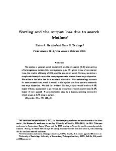
Sorting and the output loss due to search frictions Pieter A. Gautieryand Coen N. Teulings
z
February, 2011
Abstract We analyze a general search model with on-the-job search and sorting of heterogeneous workers into heterogeneous jobs. This model yields a simple relationship between (i) the unemployment rate, (ii) the value of non-market time, and (iii) the max-mean wage di¤erential. The latter measure of wage dispersion is more robust than measures based on the reservation wage, due to the long left tail of the wage distribution. We estimate this wage di¤erential using data on match quality and allow for measurement error. The estimated wage dispersion and mismatch for the US is consistent with an unemployment rate of 4-6%. We …nd that without search frictions, output would be between 7.5% and 18.5% higher, depending on whether or not …rms can ex ante commit to wage payments. JEL codes: E24, J62, J63, J64
We thank seminar participants at MIT, the 2009 Sandjberg conference on search models of the labor market, and the Sciences Po conference on sorting for useful comments and discussions. Finally, we thank Bart Hobijn for sharing his labor-market ‡ow data with us. y VU University Amsterdam, Tinbergen Institute, CEPR, Ces-Ifo, IZA, email:
[email protected] z Netherlands Bureau of Economic Policy Analysis, University of Amsterdam, Tinbergen Institute, CEPR,.CeS-Ifo, IZA, email:
[email protected]
1
Introduction
Relative to a competitive economy, an economy with search frictions generates less output because (i) there are idle resources like unemployed workers, (ii) resources are spent on recruitment activities, and (iii) the assignment of workers to jobs is sub-optimal. Heterogeneity is crucial when assessing the importance of search frictions. If all unemployed workers and jobs were alike, it would be hard to imagine why it would take workers months to …nd a good match. The more important the quality of the match, the costlier are search frictions. This paper analyses a class of search models with on-the-job search (OJS) and heterogeneity among workers and jobs. As a starting point, we take the framework of Gautier, Teulings, and Van Vuuren (2010) where the productivity of a match is decreasing in the distance between worker and job type and where employed workers continue moving towards the most productive jobs. We use a production technology that can be interpreted as a second order Taylor approximation of a more general production function. Within this framework, various wage mechanisms can be analyzed like wage posting with full commitment as in Burdett and Mortensen (1998) and wage mechanisms without commitment as in Coles (2001) and Shimer (2006). The key di¤erence between wage setting with and without commitment is that in the …rst case, …rms pay both hiring and no quit premia to hire/ keep workers whereas in the latter case, the only reason for …rms to pay workers above their reservation wage is to prevent them from quitting. The equilibrium is characterized by a relationship between just three statistics: (i) the unemployment rate, (ii) the value of non-market time, and (iii) a summary statistic for wage dispersion between identical workers, the max-mean wage di¤erential. We show that this statistic is more informative and more robust than alternatives like the ratio of the mean wage to the reservation wage (i.e. the mean-min ratio of Hornstein, Krusell and Violante, 2010). This relation hardly depends on any of the model’s parameters, except for the relative e¢ ciency of on- versus o¤-the-job search,
. For the calculation of the total output loss
due to search frictions for a given unemployment rate, even the e¤ect of
is a higher
order phenomenon. The combination of two-sided heterogeneity and search frictions relates our model 1
to the literature on hedonic pricing in the spirit of Rosen (1974), Sattinger (1975) and Teulings (1995,2005). These models are hierarchical, in the sense that better skilled workers have a comparative advantage in more complex jobs. Hence, there is a least and a best skilled worker, and there is a least and most complex job type. In a Walrasian equilibrium, there is perfect sorting. With search frictions, this perfect correlation between worker and job types breaks down, since workers cannot a¤ord to wait for ever till the optimal match comes along. Shimer and Smith (2000) and Teulings and Gautier (2004) are early examples of assignment models with search frictions. Hierarchical models are di¢ cult to solve because matching sets in the corners of the type space do not have interior boundaries. We therefore …rst transform the hierarchical model into a circular model in the spirit of Marimon and Zilibotti (1999) and Gautier, Teulings, and Van Vuuren (2008). The idea is that pro…ts are decreasing in the distance between worker and job types. This makes it possible to derive a closed form solution of the equilibrium. When turning to the empirical analysis of data on individual wages, and on worker and job characteristics, we reintroduce the hierarchical aspect of the model. Ultimately, the usefulness of our model depends on how well it can simultaneously describe the observed wage dispersion due to mismatch, the unemployment rate, and the ratio of job-to-job versus unemployment-to-job worker ‡ows. We show that the equilibrium unemployment rate in our model that is consistent with the observed amount of wage dispersion is between 4% and 6% which seems reasonable. Given that our model performs well, we can calculate the total output loss due to search frictions which is between 8% and 12% if …rms can commit to wage payments, and between 14.5% and 18.5% if they cannot. The majority of the output loss is due to recruitment activities and mismatch. Hornstein et.al. (2010) also derive a simple relationship between the unemployment rate and wage dispersion that holds for a large class of search models. They argue that search models without OJS cannot explain the coexistence of low unemployment rates and substantial wage dispersion because the …rst suggests low frictions and the latter suggests high frictions. Gautier and Teulings (2006) made the related point that without OJS, estimates of output losses due to search frictions based on the unemployment rate are substantially lower than estimates based on wage dispersion. Allowing for OJS and
2
unobserved heterogeneity can resolve this issue. OJS lowers the reservation wage which increases wage dispersion for a given unemployment rate. As in Hornstein et al. (2010) this requires a su¢ ciently large contact rate for employed workers. . Similarly, Eeckhout and Kircher (2010) construct a measure based on the distance between the lowest and highest wage. One disadvantage of relating wage dispersion to the lowest observed wage (see also the mean-min ratio of Hornstein et.al.,2010) is that the wage distribution for a given skill type has a long left tail. This long tail is consistent with OJS for the reasons spelled out in Burdett and Mortensen (1998): (i) OJS reduces the lowest acceptable job type because less option value of continued search has to be given up when accepting a job, and (ii) less workers quit from good matches and more workers accept good matches. Empirically, it matters a lot whether one takes the 1th or the 2nd percentile of the wage distribution as a proxy for the reservation wage. Therefore, the di¤erence between the highest wage at the optimal assignment and the mean wage (the max-mean di¤erential) is a more robust measure for wage dispersion. When on- and o¤-the-job search are equally e¢ cient and when the well known congestion e¤ects of opening vacancies are switched o¤ (i.e. by a quadratic contact technology), the equilibrium where …rms are able to commit to their posted wages is constrained ef…cient. In the equilibrium where …rms are unable to commit, quasi-rents per worker are higher than in the social optimum due to a business-stealing externality. Under free entry, these quasi-rents are spent on (excess) vacancy creation, see Gautier, Teulings and van Vuuren (2010). We estimate the output loss due to this business externality to be up to 6% (if no …rm commits). The empirical estimate of the max-mean wage di¤erential for identical workers in heterogeneous jobs is an extension of the framework of Gautier and Teulings (2006) with OJS. Our estimate is based on the intercept of a simple quadratic wage regression with appropriately normalized measures for worker and job characteristics. This type of inference is highly sensitive to measurement error in both characteristics because an observed sub-optimal matched worker can either re‡ect true mismatch, or simply imply measurement error. Our estimation procedure accounts for this problem. Gautier and Teulings (2006) use second order terms in worker and job characteristics to capture the concavity
3
of wages around the optimal assignment that is implied by search models with sorting. However, there is a crucial di¤erence between a model with and without OJS. In a model without OJS, wages are a linear transformation of the match surplus. Since the match surplus is a di¤erentiable function of the match quality indicator, so is the wage function. This simple relation no longer applies with OJS, see Shimer (2006). The wage function turns out to be non-di¤erentiable at the optimal assignment. At that point, …rms are prepared to pay the highest premiums to raise hiring and to reduce quitting. In our empirical application, we take this into account. Allowing for OJS is important since Fallick and Fleischman (2004) and Nagypal (2005) show that job-to-job ‡ows are substantial. Lise, Meghir and Robin (2008) and Lopes de Melo (2008) also look at sorting in models with OJS. Their focus is on interpreting the correlations between worker and …rm …xed e¤ects and how this relates to complementarities between worker and job types in the production technology. Finally, Eeckhout and Kircher (2009) consider a simple model based on Atakan (2006) where workers and jobs are randomly matched and have the option to dissolve and at some cost move to a competitive sector with perfect sorting. They derive a similar hump shaped relation where productivity is highest at the optimal assignment and decreases in the distance from this optimal assignment. This framework is however less suitable to bring to the data. The structure of the rest of this paper is as follows. Section 2 presents the basic framework. Section 3 discusses the basic steps in our argument. In this section, we also reinstall the hierarchical features of the model and derive the wage function that comes with it. We also show how we can normalize worker and job skills such that we can relate the constant in a simple wage regression to the max-mean wage di¤erential. Finally, section 4 concludes.
2 2.1
The model Why a circular model?
Shimer and Smith (2000) and Teulings and Gautier (2004) analyze an assignment model with search frictions and without OJS. Though the idea is straightforward, the analysis
4
is complicated. Figure 1 provides an intuition for why this is the case. The …gure shows the space of potential matches between skill types, s; and worker types, c. The Walrasian equilibrium assignment is depicted by the main diagonal. Comparative advantage of skilled workers in complex jobs implies that it is upward sloping. Perfect sorting implies that it is a one-to-one correspondence. Search frictions and su¢ cient complementarities between worker and job types imply that the equilibrium assignment is a set rather than a point where x measures the distance of worker type s to her optimal assignment. Away from the corners, the optimal match is in the middle of the matching set while close to the corners, the optimal assignment is close to the boundary. Teulings and Gautier (2004) who do not allow for OJS use Taylor expansions for the middle part and show that for small search frictions and if worker and job types are normally distributed, the corner problem can be ignored. With OJS this approach does not work well. Gautier, Teulings, and Van Vuuren (2005) show that by taking out the hierarchical aspect of the model, the south-west and the north-east corner of the matching space can be "glued" together. Then, a circular model in the spirit of Marimon and Zilibotti (1999) can be used, see the lower part of Figure 1. The distance x to the optimal assignment is now measured along the circumference of the circle. All conclusions from the analysis of the hierarchical model without OJS in Teulings and Gautier (2004) based on Taylor expansions carry over to the circular model. The intuition for this is that if there is relatively little mass around the corners, all that matters for productivity is the distance to the optimal job. We follow this idea in this paper, but now for a model with OJS. First, we take out the hierarchical feature and provide a closed form analysis of a search equilibrium with sorting in the context of the circular model. Then, we reintroduce the hierarchical aspect for the empirical analysis of wage di¤erentials, using data with information on worker and job characteristics, which are hierarchical by nature. The interpretation of the circular search model as an approximation of the hierarchical model has an important implication for the production structure. Consider Rosen’s (1974) Hedonic equilibrium in the wage-skill space. The reservation wage is increasing in worker’s skill type and all values of s enveloped by this reservation wage and the …rm’s o¤er curve are now part of the matching set of that job type. Taking out the hierarchical aspect of the model implies that the (reservation)
5
c
x s
c x s
Figure 1: The hierarchical versus the circular model
wage function becomes horizontal. What is crucial is that these functions keep their shape by this operation. Hence, these functions are di¤erentiable in their maximum. We impose this feature in the theoretical model.
2.2
Assumptions
Production There is a continuum of worker types s and job types c; s and c are locations on a circle. Workers can only produce output when matched to a job. The productivity of a match of worker type s to job type c depends on the "distance" jxj between s and c along the circumference of the circle, where x is de…ned as x
s c. Y (x) has an interior maximum
at x = 0; it is symmetric around this maximum, which is normalized to unity: Y (0) = 1; Y (x) is twice di¤erentiable and strictly concave. We consider the simplest functional form that meets these criteria: Y (x) = 1 x is the mismatch indicator. The parameter
1 2 x: 2
(1)
determines the substitutability of worker
types. Y (x) can be interpreted as a second order Taylor approximation around the optimal assignment of a more general production technology. Since, the …rst derivative of a continuous production function equals zero in the optimal assignment, Y 0 (0) = 0, the 6
…rst order term drops out. We are interested in equilibria where unemployed job seekers do not accept all job o¤ers, which imposes a minimum constraint on .1 Labor supply and the value of non market time Labor supply per s-type is uniformly distributed over the circumference of the circle. Total labor supply in period t equals L(t). Unemployed workers receive the value of non market time B. Employed workers supply a …xed amount of labor (normalized to unity) and their payo¤ is equal to the wage they receive. Workers live for ever. They maximize the discounted value of their expected lifetime payo¤s. Labor demand There is free entry of vacancies for all c-types. The cost of maintaining a vacancy is equal to K per period. After a vacancy is …lled, the …rm’s only cost is the worker’s wage. The supply of vacancies is determined by a zero pro…t condition. Vacancies are uniformly distributed over the circumference of the circle; v (c) = v is the measure of vacancies per unit of c. Job search technology We use a reduced form speci…cation of the job search technology: =
(u; v) ;
v
> 0;
and assume that the rate at which unemployed workers meet jobs is
and the rate at
which employed workers meet jobs is
1; measures the
:The parameter
relative e¢ ciency of on- relative to o¤-the-job search;
;0
= 0 is the case without OJS; for
= 1, on- and o¤-the-job search are equally e¢ cient. When a worker quits her old job, this job disappears. Job destruction Matches between workers and jobs are destroyed at an exogenous rate
> 0.
Golden-growth path 1
A su¢ cient condition for this is that Y (x) < 0 for at least some x. Let C be the circumference of the circle, then 0 x 21 C. Hence > 8C.
7
We study the economy while it is on a golden-growth path, where the discount rate
>0
is equal to the growth rate of the labor force. We normalize the labor force at t = 0 to one. Hence, the size of the labor force is L(t) = exp( t). The assumption of a golden-growth path buys us a lot in terms of transparency and tractability. The implications of the golden growth assumptions are equivalent to those that follow from the assumption that the discount rate
converges to zero, an assumption that is often applied in the wage
posting literature, see for example Burdett and Mortensen (1998) because discounting reduces future output while population growth increases it. New workers enter the labor force as unemployed. Labor supply per worker type and the productivity in the optimal assignment Y (0) are normalized to one. Hence, in the absence of search frictions, the output of this economy equals one. Wage setting Wages, denoted by W (x), are set unilaterally by the …rm, conditional on the mismatch indicator x in the current job. We analyze wage setting under two di¤erent assumptions. Under the …rst assumption, …rms can commit to a future wage payment contingent on x. Then, …rms pay both no-quit and hiring premiums, that is, they account for the positive e¤ect of a higher wage o¤er on reduced quitting and increased hiring. Under the second assumption, …rms are unable to commit to future wage payments. In this case, hiring premiums are non-credible because immediately after the worker has accepted the job, the …rm has no incentive to continue paying a hiring premium, since the worker cannot return to her previous job. Workers anticipate this, and will therefore not respond to this premium in the …rst place, and hence, …rms will not o¤er it. No-quit premiums are credible even without commitment because it is in the …rm’s interest to pay them as soon as the worker has accepted the job.2 2
See also Bontemps van den Berg and Robin (2000) for wage setting with and Coles (2001) and Shimer (2006) for wage setting without commitment.
8
2.3
The asset values of (un)employment and vacancies
The golden-growth assumption is particularly useful for the derivation of the asset values of employment, unemployment, and vacancies. Asset value of unemployment The asset value of unemployment, denoted by V U is a weighted average of the worker’s payo¤ while unemployed, B, and the expected wage when employed, Ex W , the weights being the unemployment and the employment rate, respectively: V U = uB + (1
u) Ex W:
(2)
The derivation of this and the subsequent Bellman equations can be found in the technical appendix A.1 to this paper. Why does this relation take such a simple form? The reason is that the growth rate of the workforce is equal to the worker’s discount rate. Therefore, the expected payo¤ of a worker with one year of experience is equal to the average payo¤ of the cohort of workers that entered the labor force one year ago. Likewise, the expected payo¤ of a worker with two years of experience is equal to the average payo¤ of the cohort of workers that entered the labor market two years ago, etc. The asset value of unemployment is equal to the weighted sum of expected payo¤s for each level of experience, future payo¤s being discounted at a rate
per year. This weighted sum is exactly equal to
the sum of payo¤s for the current workforce. The fact that older cohorts are smaller than younger cohorts due to the growth of the labor force at a rate
exactly o¤sets the e¤ect
of discounting future payo¤s for the calculation of the asset value of unemployment. The term (1 when
u)Ex W can be interpreted as the option value of …nding a job. Alternatively, ! 0, workers spend a fraction u of their life as unemployed and the rest of the
time they are employed.
Asset value of employment in the marginal job Let V E (x) be the asset value of holding a job with mismatch indicator x. At x, an unemployed job seeker is indi¤erent between accepting the job or waiting for a better o¤er: V E (x) = V U . Again, the asset value for this job is a weighted average of W (x)
9
and Ex W , V E (x) =
uW (x) + (1 u + (1
u) Ex W ; u)
The factor u +
(1
seekers and (1
u) employed job seekers, which are discounted by a factor
(3)
u) is the e¤ective supply of job seekers, namely u unemployed job due to their
lower search e¤ectiveness. Hence, the weights in equation (3) are the shares of unemployed and employed respectively in the e¤ective supply. The intuition for this equation is that the option value of …nding a better job is the same as for an unemployed job seeker, since both an unemployed and a worker employed in the marginal job type x = x accept any job: 0
jxj < x. However, the option value of an employed worker is only a fraction
of the option value of an unemployed due to their lower contact rate. The value of non market time B does not show up in the equation since V E (x) = V U which implies that we can substitute V E (x) for V U , thereby eliminating B from the equation. For 0 <
< 1,
unemployed job seekers give up part of the option value of search by accepting a job and they need to be compensated for this, implying that W (x) > B. For
= 1, on- and
o¤-the-job search are equally e¢ cient. Asset value of vacancies Adding up the zero pro…t condition for all vacancies implies that the total cost of maintaining vacancies must be equal to the aggregate rents that …rms make in currently …lled jobs. vK = (1
u) (Ex Y
Ex W ) :
(4)
The left hand side of this equation is the total cost of vacancies at t = 0. The right hand side is employment 1
u times the quasi-rents per worker, which is equal to expected
output Ex Y minus expected wages Ex W . The reservation value of the mismatch indicators The de…nition of x as the mismatch indicator of a job which is just acceptable to an unemployed job seeker implies: W (x) = Y (x) = 1
10
1 2 x; 2
(5)
Substitution of equation (2) and (4) in the condition V E (x) = V U yields, W (x) = [u +
(1
u)] B + (1
) (1
When on and o¤ the job search are equally e¢ cient, W (x) = B = 1
u) Ex W:
(6)
= 1, equation (6) simpli…es to:
1 2 x: 2
(7)
where the last step follows from (5). Hence, the relation between
and x does not
depend on expected wages in this case, and consequently neither on whether or not …rms can commit on paying hiring premiums. The output loss due to search frictions The de…nition of the output loss due to search frictions is given by: X = (1
u) (1
Ex Y ) + u (1
B) + vK = 1
The output loss is equal to employment, 1
(1
u) Ex Y
uB + vK:
(8)
u; times the di¤erence between productivity
in the optimal assignment, Y (0) = 1, and the expected productivity in the actual assignment, Ex Y , plus unemployment, u; times the di¤erence between the productivity in the optimal assignment and the value of non market time, 1
B, plus the cost of keeping
vacancies open, vK. Substitution of equation (2) and (4) in (8) yields: X=1
V U = u (1
B) + (1
u) (1
Ex W ) :
(9)
The last step follows from the fact that by the zero pro…t condition, the cost of maintaining vacancies is equal to the surplus of expected productivity over expected wages, see equation (4). The …rst equality tells us that the output loss is equal to the output in the optimal assignment (Y (0) = 1) minus the asset value of unemployment. The second equality in (9) tells us that the output loss is equal to the sum of the output loss for unemployed and for employed workers. The former is equal to the lost output in the optimal assignment minus the value of non market time, while the latter is equal to the foregone wage income. Under free entry, the di¤erence between wages and productivity is spent on vacancies.
11
2.4
Equilibrium ‡ow conditions
Under both assumptions for wage setting, commitment and no-commitment, wages are a decreasing function of x for x
0, Wx (x) > 0, implying that workers accept any job-o¤er
with a lower mismatch indicator jxj than their current job. Hence, we can analyze jobto-job ‡ows independent of the exact form of the wage policy W (x). Let G(x); x
0, be
the fraction of workers employed in jobs at smaller distance from their optimal job than jxj. This implies that G (0) = 0 and G (x) = 1, since x is the largest acceptable value of
jxj. The golden growth assumption requires that the number of workers employed in jobs with a mismatch indicator lower than x grows at a rate : 2 x fu + (1
u) [1
G (x)]g
(1
u)G (x) = (1
u)G (x) :
(10)
The …rst term on the left-hand side is the number of people that …nd a job with mismatch indicator lower than x, either from unemployment (the …rst term in braces), or by mobility from jobs with a larger mismatch indicator (the second term in brackets). The number of better jobs is given by 2x, since the worker can accept jobs both to the left and to the right of her favorite job type x = 0. The second term in brackets is weighted by the factor , re‡ecting the e¢ ciency of on- relative to o¤-the-job search. The …nal term on the lefthand side is the out‡ow of workers due to job-destruction. The right-hand side re‡ects that at the balanced growth path, employment grows at a rate
at all levels including
the class of workers with a mismatch indicator smaller than x, G (x). Mobility within this class is irrelevant because the disappearance of the old match and the emergence of the new one cancel. Evaluating (10) at x and solving for u yields, 1 ; (11) 1+ x : VOETNOOT OVER KAPPA=1 Substitution of (11) into condition (10) u=
where:
2 +
gives, G (x) = 1
2.5
x (1 +
x 1+ ; g (x) = x) x x (1 +
x : x)2
(12)
Wage formation
The wage formation processes are the same as in Gautier, Teulings, and Van Vuuren (2010). Since the model is symmetric around x = 0, we can focus on the analysis of 12
W (x) for x
0.
Wage setting with commitment When …rms can commit on future wage payments, the optimal wage policy of the …rm maximizes the expected value of a vacancy, W (x) = arg max W
b [W (x)] where G where F [W (x)]
h
u+
(1
i b (W ) u) G
Y (x) + +
W F (W )
;
(13)
G (x) is the distribution of wages among employed workers and
1 x x
is the wage o¤er distribution, using the fact that the distribution b (W ) on the optimal wage o¤er is the hiring of x is uniform by assumption. The e¤ect of G 1
premium, the e¤ect of F (W ) is the no-quit premium. The …rst order condition of this
problem reads:
Wx (x) =
2
1+
x
[Y (x)
W (x)] :
(14)
This di¤erential equation can be solved analytically for W (x), using equation (5) as an initial condition, see Appendix A.4. Wage setting without commitment When …rms cannot commit on future wage payments, hiring premiums are non-credible b (W ) in equation (13) is replaced by 1 G (x) re‡ecting that the and. Hence, the term G …rst term in brackets does not depend on the wage and that the wage maximizes the value of a …lled job rather than the value of a vacancy. Then, the …rst order condition reads, Wx (x) =
1+
x
[Y (x)
W (x)] :
(15)
The only di¤erence with equation (14) is a factor two, re‡ecting the fact that …rms pay hiring and no quit premia in the case of commitment, while they pay only a no quit premium in the case without commitment. Again, an analytical solution for W (x) is available, see Appendix A.4.
2.6
Characterization of the equilibrium
The shape of the wage function
13
y
1.0 0.9 0.8 0.7 0.6 0.5
-20
-10
0
10
20
x
Figure 2: Productivity Y (x) (thick) and wages W (x) with (thin) and without (dotted) commitment
Figure 2 depicts Y (x) and W (x) both for the case with and without commitment, setting the value of non market time at B = 0:4 (which we do in all subsequent plots).3 Contrary to Y (x), W (x) is non-di¤erentiable at x = 0. This is due to the hiring and no-quit premiums that …rms pay. Since the density of employment is highest for low values of jxj, the elasticity of labor supply is high for these types of job. A slight variation
in wages has large e¤ects both on the probability that workers accept an outside job o¤er and on the number of workers who are prepared to accept the wage o¤er (the latter being relevant in the case with commitment only). Hence, …rms will bid up wages aggressively for these types of jobs. Figure 2 shows that the wage in the optimal assignment is higher when …rms can commit than when they cannot, since the ability to commit increases competition between …rms for workers. Figure 2 also reveals that for x = 0 the slope of the wage function is smaller (in absolute value) for the case with than without commitment. This is remarkable, since the only di¤erence between the expressions for the slope is a factor 2 in the di¤erential equations for wages for the case with commitment, compare equation (14) and (15). However, the slope is proportional to the ‡ow pro…ts per worker, i.e. the di¤erence 3
Hagedorn and Manovskii (2008) and Hall (2009) want to explain the cyclical behavior of unemployment so they use larger values for B. For these studies, the value of non-market time of the marginal worker is relevant whereas here we are interested in the value of non-market time for the average worker so a lower value of B is justi…ed.
14
g(x), G(x)
1.0
0.8
0.6
0.4
0.2
0.0 0
2
4
6
8
10
12
14
16
18
x
Figure 3: The distribution (thick black) and density function (thin red) of x conditional on employment
between the productivity and wages, Y (x)
W (x) which is more than twice as large
in the case without commitment. The latter e¤ect dominates yielding a steeper wage function in that case. The distribution of x among employed Figure 3 depicts the density and distribution function of the mismatch indicator jxj
conditional on employment, for the case u = 4%;
= 1 and
= 1 (we use these values
in all subsequent plots, unless stated otherwise). For a given unemployment rate, G(x) is identical with or without commitment since workers climb the job ladder equally fast in both cases (because wages are in both cases strictly decreasing in x). The main message from Figure 3 is that the distribution of jxj has a large probability mass close to zero (the optimal assignment) and a long right tail of bad matches. The median value of x is equal
to (1
u)=(1 + u) < 1, far smaller than x = (1
u)=u = 24:0 (the mismatch indicator
in the worst match). The reason for this pattern is that workers who are matched badly quit their jobs fast. The reverse holds for good matches, so their density is high. The skewness of the distribution of jxj has a number of counter intuitive implications for the wage distribution that are spelled out in greater detail below.
15
The impact of
on wage di¤erentials and the loss due to search frictions
The max-mean and the mean-min wage di¤erentials are depicted in Figure ?? for the case with commitment together with the output loss due to search frictions. Contrary to the mean-min di¤erential, the max-mean di¤erential is largely independent of
, while
the mean-min di¤erential is very sensitive to the precise value of . For the case without commitment (not in the Figure) the max-mean di¤erential varies even less with
. It is
important to realize that this is not a comparative statics exercise in , for then it would not make sense to keep u constant. The question addressed here is what wage di¤erential and output loss are consistent with a particular value of of 4%. Implicitly, the value of The reason why the value of
and an unemployment rate
adjusts to keep the unemployment rate at this level.
does not matter for the max-mean wage di¤erential is that lowering
while keeping u constant has two o¤setting e¤ects on wage di¤erentials
near the optimal assignment. The density of x at the optimal assignment is equal to g (0) =
u), see equation (12). Hence, a lower value of
+ u=(1
implies that there
are fewer workers close to the optimal assignment since search by employed workers is less e¢ cient and since employed job seekers are a particularly relevant source of labour supply for an x = 0. This reduces the mean wage. Therefore, holding W (x) constant, a lower value of
yields a larger max-mean wage di¤erential. However, holding x constant,
unemployed job seekers become more choosy if
goes down since they give up a share 1
of the option value of search by accepting a job. Therefore, the lowest wage W (x) increases a lot and consequently the mean wage increases a bit as well; the total e¤ect is that wage di¤erentials become smaller. For the mean-max di¤erential, the negative and positive e¤ects on the mean wage almost cancel while the maximum wage is una¤ected. Hence, contrary to the max-mean di¤erential, the mean-min di¤erential is particularly sensitive to the value of
. The output loss due to search frictions is again largely insensitive to
. The reason is that when
< 1 unemployed reject some job o¤ers that are only only
marginally more productive than the value of leisure. Whether or not unemployed accept these jobs does not matter much for the output loss, since their contribution to output is marginal anyway. The max-mean di¤erential on the one hand and the mean-min and max-min wage
16
di¤erentials on the other hand tell opposite stories about the e¤ect of commitment on wage di¤erentials. Commitment makes …rms compete more …ercely for workers, driving up the maximum wage. Since the minimum wage is the same for the case with and without commitment, this would imply that the max-mean di¤erential is larger under commitment. However, since the slope of the wage function close to the optimal assignment is smaller under commitment, see Figure 2, the max-mean di¤erential is actually smaller; 5:6% of the wage in the optimal assignment with commitment versus 8:8% without commitment. Wrapping up Both versions of the model -commitment and no commitment- yield two analytical relations between expected wage and productivity losses due to search frictions on the one hand and the parameters B and W (0) Y (0)
and the unemployment rate u on the other hand:
f (u; B; ) ; Ex W = W
Ex Y = Ye (u; B; ) =
(16) 1 Var [x] ; 2
where W (0) Ex W is the expected wage loss compared to the wage in the optimal assignment, W (0), and mutatis mutandis the same for Y . HIER IS EEN TERMINILOGIE PROBLEEM: ALS WE SPREKEN OVER DE OUTPUT LOSS DOOR SEARCH FRICTIES DAN GEEFT DAT VERWARRING MET DE EERDER GEDEFINIEERDE X. MISSCHIEN KUNNEN WE DAT BETER DE WELFARE LOSS NOEMEN EN Y (0)
Ex Y DE OUTPUT LOSS These relations are presented in Appendix A.4. Both
relations are increasing in u for both version of the model. Hence, keeping B and constant, there is an increasing relation between wage di¤erentials W (0) Ex W and the output loss Y (0) Ex Y : d [W (0) d [Y (0)
fu (u; B; ) Ex W ] W = > 0: Ex Y ] Yeu (u; B; )
(17)
A higher unemployment rate goes hand in hand with both higher wage di¤erentials and a larger output loss. When empirical estimates of either W (0) Ex W or Y (0) Ex Y are available and when we are prepared to make assumptions on B and
, we can calculate
the unemployment rate u as predicted by the model. If this unemployment rate were consistent with its natural rate, we would consider that as a strong support for the model. 17
In what follows, we will use wage data to obtain estimates of both W (0) Ex W and Var[x]. Moreover, we apply information on
from other sources. This enables us to put the model
to a test. Before doing that, we discuss some peculiarities of the market equilibrium of this model.
3
Using the hierarchical model calibration
3.1
The hierarchical model and the value of
The advantage of the hypothetical world of the circular model is that it allows a full analytical characterization of the equilibrium of the search. However, for empirical inference, the circular model is too far from reality. In the real world, workers di¤er by their human capital. Better skilled workers earn higher wages. They are likely to have a comparative advantage in more complex jobs. Having a PhD in …nance is not much of an advantage when working as a brick layer. It is a major advantage when working at Wall Street. Or more general: better skilled workers have a comparative advantage in complex jobs. Since the labor market tends to sort people into jobs where their human capital yields the highest return, the human capital of somebody having a PhD in …nance is likely to pay o¤. A full ‡edged model with hierarchy, search frictions, and on-the-job search is analytically untractable. However, a full analytical characterization of the circular model.is equivalent to a Taylor expansion of the a hierarchical model, see Teulings and Gautier (2004) for a search model without on-the-job search. VOETNOOT OVER DE UNIFORMITEITSVERONDERSTELLING BIJ DE VACANCY VERDELING, MOETEN WE MEER ZEGGEN OVER DE PERFECTE ANALOGY, BIJVOORBEELD HOE FIGUUR XX IN DE BEGIN SECTIE VERDRAAID WORDT VANUIT HET GEZICHTSPUNT VAN EEN BEDRIJF C OMDAT WELISWAAR DE OUTPUT EEN STIJGENDE FUNCTIE IS VAN S MAAR DE KOSTEN OOK, DUS DAT HET CIRCULAIRE BEELD PRECIES?? MOETEN WE UITLEGGEN DAT ONZE BENADERING GELDT VOOR KLEINE FRICTIES? Hence, we leave the hypothetical hierarchical world and enter the more realistic world
18
of a hierarchical labour market. Apart from the empirical realism, entering the hierachical world brings us a further advantage. For the derivation of a value for , the interpretation of the circular model as a simpli…ed representation of an hierarchical assignment model allows us to draw an analogy to the theory of imperfect substitution between low and high skilled workers, see Teulings (2005) and Teulings and Van Rens (2008). In fact, measures the curvature of Rosen’s "kissing" o¤er and utility curves, see Figure XX. We can establish a relation between our estimation results and the elasticity of substitution between low and high skilled. Let Y (s; c) denote the productivity of an s-type worker in a c-type job. Instead of equation (1), let this productivity satisfy the following relation: ln Yb (s; c) = s
1 (s 2
c)2 ;
(18)
where put a hat above the function to distinguish it from the single argument function (1) of the circular model. Now, a worker of skill type s has both a comparative advantage in a job-type of the same complexity c as her skill level s and an absolute advantage over other workers with a lower skill, so that he receives a higher wage than these workers when employed in his optimal assignment.4 The …rst term captures the absolute advantage of better skilled workers (the hierarchical aspect of the model). The second term captures the match quality. Its speci…cation is equivalent to the circular model in equation (1), in the sense that: Y 00 (0) =Y (0) = Ybcc (c; c) =Yb (c; c) = ; this parameter is comparable to in equation (1). The log supermodularity of Yb (s; c) is su¢ cient for positive assortative
matching in a Walrasian equilibrium, see Teulings (1995). The optimal assignment c (s) of 4
Absolute advantage of better skilled workers applies only locally for this speci…cation, since for high values of s the second order term dominates. Teulings and Gautier (2004) use the production function: ln Y (s; c) =
1
e
(s c)
+ ln P (c) ;
where P (c) is the price of output of type c. This price depends on the distribution of s among skill supply and the distribution of c among product demand. This function features global absolute advantage: Ys (s; c) > 0 for any s and c. Equation (18) can be interpreted as a second order Taylor expansion of this relation in the market equilibrium where s = c, or equivalently, where ln P (c) = c 1: ln Y (s; c) = 1 + (s
c)
19
1 (s 2
2
c) + ln P (c) ;
worker type s maximizes the market value of her output. The …rst order condition for this problem, Ybc (s; c) = 0, implies c (s) = s or x = 0. In the Walrasian equilibrium, everybody
is assigned to her optimal c-type and the second term vanishes. At …rst sight the linearity of equation (18) in s seems to be a serious limitation to its generality. However, Gautier and Teulings (2006) show that it is not. Since we have not yet de…ned the units of measurement of s yet, the linearity of the …rst term is just a matter of proper scaling of the skill index. Hence, the restrictive nature of equation (18) is not in the …rst but in the second term, namely that the coe¢ cient of the second term, , does not vary with s.5 By a similar argument, the fact that equation (18) is constructed such that the optimal assignment is characterized by the simple identity c (s) = s instead of a more general function, is not a restriction to the model, but just a matter of proper scaling of the complexity index c. Implicitly, equation (18) de…nes the units of measurement of s and c, and hence of x = s
c: optimal assignment, where x = 0 and hence s = c, the Mincerian
return to the skill index d ln W=ds is equal to unity. Later on, we use this normalisation when constructing our measures for s and c. In our discussion of the model, we keep constant the distribution of worker-skills and job-complexities at such a level that the Mincerian rate of return to the skill index is equal to unity and that the optimal assigment of worker type is c (s) = s. In reality, the distribution of s and c might shift over time or di¤er between regions. For example, when the average skill level of the workforce increases over time while the distribution of product demand over c-types remains constant, the equilibrium between demand and supply of each c-type requires the optimal assignment and the Mincerian to adjust: workers of a particular s type will be assigned to less complex jobs and the Mincerian rate of return to skill will go down. The formal derivation of this argument is relegated to Appendix A.6. This relates our model to the literature on the change relative wages due shifts in the distribution of human capital, in particular Katz and Murphy (1992). They estimate the elasticity of complementarity between high and low skilled workers
low-high
to be 1.4:
1 % increase in the ratio between high and low skilled workers yield 1.4% fall in the relative wages of high skilled workers. In Appendix A.6 we show that there is a one to 5
Teulings (2005) refers to this case as the constant complexity dispersion equilibrium.
20
one correspondence between this elasticity 1 Var [ln W ]
= The fact that the parameter
low-high
= low-high
and the parameter : 1
0:36
1:4
= 2;
is related to the elasticity of complementarity should not
come as a surprise. Elasticities of complementarity are a function of the second derivative of production function, and that is exactly what
is:
measures the curvature of Rosen’s
kissing curves.
3.2
and B
The value of
PIETER, IK VIND HET ONDERSTAANDE ARGUMENT NIET HELDER OPGESCHREVEN, MAAK JIJ DAT SCHERPER In the technical Appendix A.3 we derive a relation between the ratio of the employmentto-employment, fee ; and the unemployment-to-employment-hazard rate, fue s fee u u + (1 u) ln = fue 1 u (1 u)
1
u
1 :
(19)
Unfortunately, the evidence on fee and fue for the US yields values of
that range from
u
+1
above 1, see Nagypal (2008), to values close to 0, see Hornstein et.al. (2010). What explains this wide range?
6
Hornstein et al. (2011) use Shimer’s (2005) estimate (that
corrects for time aggregation) of the employment-to-unemployment hazard rate feu , which equals 3%. The problem of this high value of feu is that according to the BLS statistics, median tenure is 53 months. Without accounting for duration dependence and ignoring the ‡ow out of the labor forces, this implies that the total hazard out of the current job, fee + feu , is 1.3%:7 At …rst sight, the di¤erence between this estimate and Shimer’s can 6
The value of fee is 2.7% according to Fallick and Fleischman (2004), 2.9% according to Nagypal and after a correction for missing records in the CPS, Moscarini and Vella (2008) get a value of 3.3%. Nagypal’s values come from the SIPP and the CPS. She argues that those estimates are downwardly biased because when workers …nd a new job when employed but there is a lag in starting this new job, it is not uncommon to brie‡y register to be unemployed. In the data this implies an employmentunemployment transition followed by an unemployment-employment transition. She argues that this bias is larger than the time aggregation bias in the unemployment out‡ow rate (some workers loose and …nd a job between the interview dates). 7 Ignoring ‡ows out of the labor force, the total hazard outof employment can be solved from 1 exp [ 53 (fee + feu )] = 0:5:
21
be readily explained by negative duration dependence. Negative duration dependence implies that the hazard rate for low-tenure workers is above 1.3% and the rate for high tenure workers is below 1.3%. The average hazard rate is then higher than 1.3%. The theoretical model predicts negative duration dependence, since bad matches with high quit rates die out and good matches with low quite rates survive. However, in the model, the negative duration dependence is fully accounted for by the fee hazard rate. So in the data, for high-tenure workers, feu is much lower than the value reported by Shimer and for low-tenure workers it is even higher. Clearly, the model does not capture all features of reality. Apparently, a small group of weakly attached workers frequently ‡ow between un- and employment.8 In order to capture this we need other mechanisms like learning, see Moscarini (2005), or random growth, see Buhai and Teulings (2006). Since the aim of our model is to describe the behavior of the median worker, we must accept that the model is ill suited to explain the behavior of this speci…c group. Using transition rates data from (1967-2010) which are calculated in a similar manner to Shimer (2007), we obtain fue = 38%, which implies fee =fue =
2:9 38
= 0:076.9 However, if we are interested
in the median worker, the maximum value that fue can obtain is 31%:10 Together with Nagypal’s fee rate this implies, fee =fue =
2:9 31
= 0:092%. In order to mimic this ratio,
should be between 0:5 and 1: IK ZOU GRAAG VAN DIT PLAATJE AF. VALUE OF B TOEVOEGEN
4
Measuring wage di¤erentials
4.1
Inference on wages
This section describes how we can use data on wages and worker and job characteristics to construct empirical measures of s and c, and hence of the mismatch indicator x = 8
Elsby, Hobijn and Sahin (2008) show that this is a particular feature of the US labor market. Mobility rates in the other OECD countries are substantially lower. 9 We thank Bart Hobijn for sharing his data. 10 In steady state, fue = feu 1 u u where feu < 1:3%. For a frictional unemployment rate of 4% this implies that fue < 0:31:
22
fee/fue 0.12 0.10 0.08 0.06 0.04 0.02 0.00 0.0
Figure 4: Range of
s
0.2
0.4
0.6
0.8
1.0
psi
for u = 6% (fat), u = 5% (dashed), and u = 4% (thin)
c, and how we can use these data for inference on the magnitude of wage di¤erentials
W (0) Ex W . The challenging aspect of this exercise is that any empirical measure of s and c will be contaminated by measurement error. Hence, when we use these measures to construct a measure of mismatch x = s
c, the observed mismatch can be either due
to unobserved heterogeneity of either s or c, or it can really be a re‡ection of mismatch, or any combination of these two. Even in a perfect Walrasian equilibrium, we would still observe "mismatch". The observed variation in s
c therefore exceeds its true variation.
Our procedure should therefore explicitly allow for measument error. This subsection sets out the main line of the argument, using a simple approximation of the wage function as depicted in Figure xx. In the next subsection we provide numerical simulations to analyse the eact relation between our empirical statistics and the model. The wage function that goes with the production function (18) of the hierarchical model is: c (s; c) = s + ln W (s ln W
c) ;
where again we use the tilde to distinquish the this function of the single argument function of the circular model. The …rst term s measures the Walrasian, hierarchical part of the model: better skilled workers earn higher wages. The second part measures the wage loss due to search frictions as described by the function W (x) derived in Section 2. Since the function W (x) is symmetric and non-di¤erentiable around x = 0, a simple approach is to
23
estimate w (s; c) = !0 + !1 s
!2 js
(20)
cj + ";
where w denotes the log wage in deviation from its mean, where !0 > 0; !1 > 0 and !2 > 0 and where " is an error term with zero mean. Estimating this model in logs rather than levels is appropriate due to the normalization of output in the optimal assignment to unity in the circular model. Due to this normalization, Y (0) = 1, W (0) . Y (0) = 1 and hence Wx (0) = d ln W (x) =dx for small search frictions. Secondly, we apply the model in the context of an hierarchical model, where the wage in the optimal assignment depends on the worker’s skill level s. In that context, we cannot simultaneously normalize the wage in the optimal assignment for all skill levels. Estimating the model in logs resolves this problem. For the sake of the argument, we assume for the moment that perfect approximation of search frictions part of the model, ln W (s
!2 js
cj is an
c). The parameter
!2 is interpreted as an estimate of d ln W (x) =dxjx=0 = Wx (0) =W (0). The numerical simulations in the next section provides a test of the precision of this argument. We de…ne skill indexes s and c in deviation from their mean. Hence, equation (20) implies: !0 = !2 E [js
cj] & W (0)
Ex W:
The second inequality is due to Jensen’s inequality, lnEx W >Ex ln W . It applies with approximate equality for smal search frictions, and henc small wage di¤erentials, since then W (x) . W (0) . 1, so that the approximation ln W . W
1 applies. Our idea is
to use the intercept !0 as a crude estimator for W (0) Ex W . Suppose we estimate equation (20) by simply replacing x = s c by the signal x = s c. A bar on top of a variable denotes its observed part. Let "x denoted the measurement error in x, which "x is assumed to have a zero mean and to be uncorrelated to x: x = x + "x , and hence: Var[x] =Var[x] +Var["x ]. Even if ln W (s
!2 js
cj were perfect approximation of
c), the estimated value of !2 will be a biased estimator of !2 E[js
cj] due to the
strong convexity of the wage function at x = 0, since the expected value of jxj conditional on its observed part x is always greater or equal to jxj: E [jxj jx] 24
jxj :
x
3
2
1
-3
-2
-1
0
1
2
3
r
Figure 5: Smoothing of an absolute value function by random mixing for q2 = r2 = 1: jxj (thin), E[jxj jr] (thin), Taylor expansion (dashed thick), least squares estimate (thick) The close x is to zero (the point of the non-convexity), the stronger this inequality. This is documented in Figure 5, where we present four functions, jxj, E[jxj jx], a second
order Taylor expansion of E[jxj jx] at x = 0, and least squares estimation of E[jxj jx] = 0
+
1x
2
+error term, for the case that both the true value x and measurement error "x
are normally distributed with equal variance, see Appendix XX for the derivation. The second order Taylor expansion of E[jxj jx] is fairly precise for jxj < 1 while he precision of the least square approximation is excellent for a much wider range of jxj < 2:5.
This justi…es the idea of approximating the underlying model (20) by a regression
model of w with a quadratic term (s
c)2 :
w = !0 + !1s
! 2 (s
Under the assumption of joint normality of x = s
c)2 + ":
(21)
c and "x , the relation between the
structural parameter !1 and the estimated parameters !0 and !2 can be derived, see Appendix XX: !0 =
1 Var [x] 1 Var [x] !2 E [jxj] & [W (0) 2 Var [x] 2 Var [x]
Ex W ] ;
(22)
DEZE RELATIE MOET NOG GECHEKCT WORDEN First, even if x were observed without any measurement error (hence: Var[x] =Var[x] = 1), ! 0 would not be a perfect estimate of !2 E[jxj], since x2 is an imperfect approximation of jxj; ! 0 would underestimate 25
E[jxj] by a factor 2. Clearly, this underestimation can be easily corrected. The second bias is more problematic. The higher the variance of the measument error
x
the smaller the
ratio Var[x] =Var[x], and hence the smaller the estimated value of ! 0 . Hence, the share of measurement error in the variance of the observed mismatch indicator x, the more wage di¤erentials W (0) Ex W are underestimated. However, apart from the expected wage loss due to misassignment, this analysis also yields an estimate of the expected output loss compared to the optimal assignment: Y (0) Ex Y =
1 2
Var[x]. When Var[x] is used
as a proxy for Var[x], the expected output loss compared to the optimal assignment is overestimated by a factor Var[x] =Var[x], exactly the reverse of the underestimation of wage di¤erentials. Whatever the researcher tries, the empirical analysis will provide no clue about the size of this factor. However, the analysis does provide a relation between two statistices, W (0) Ex W and Y (0) Ex Y , which we use for testing the model. The situation is depicted in Figure XXX. The downward sloped function is the negative relation between W (0) Ex W and Y (0) Ex Y implied by the empirical analysis. W (0) Ex W reaches a minimum for the case that there is no measurement error in x, Var[x] =Var[x] = 1. Then, Y (0) Ex Y reaches a maximum. The higher the degree of measurement error, the higher is the implied value of W (0) Ex W , but the higher is the value of Y (0) Ex Y . The upward sloped function is the relation between W (0) Ex W and Y (0) Ex Y implied by the circular model, see equation (17). The intersection of both curves is the combination of W (0) Ex W and Y (0) Ex Y that is both consistent with the data on wages and consistent with the model. By equation (16), this intersection implies a value of the unemployment rate u. Whether the implied unemployment rate is consistent with the stylized facts about this variable provides a test to the model. HIER DE FIGUUR XXX For the construction of empirical measures for the observed part of workers’skill level s and the level of job complexity c we use a methodology spelled out in Gautier and Teulings (2006). We apply this methodology to data for the United States taken from the March supplements of the CPS 1989-1992, see Gautier and Teulings (2006), for details: w = ~x0 ~ + "s + "w ; w = ~z0 ~ + "c + "w ; 26
(23)
where ~x and ~z are vectors of observed worker and job characteristics respectively,11 where "w captures measurement error in log wages, and where "s and "c capture (i) unobserved characteristics of workers and jobs respectively and (ii) the e¤ect non-optimal assignment on wages. It is convenient to normalize our data on ~x and ~z such that they have zero mean. Since we have de…ned w to have a zero mean too, it does not make sense to include a constant in this regression. The estimated parameter vector can then be used to construct indices for the observed worker and job characteristics: s = ~x0 ~ ; c = ~z0 ~ : Again, both indices have zero mean by construction.12 So, the skill measure is the predicted wage conditional on worker characteristics and the job complexity level is the predicted wage conditional on job characteristics. The skill measures therefore satis…es our normalisation of Mincerian rate of return to skill index being equal to unity, dw=ds = 1, see equation (18). Next, we use these indices and estimate w = !0 + !s s + !c c
!ss s2 + 2!sc sc
w = !0 + !s s + !c c
!2 (s
!cc c2 + ";
(24)
c)2 + ":
The second regression imposes two restrictions !ss = !cc = !sc . At …rst sight, this equation seems inadequate to capture model (??). The model includes …rst order terms for both worker and job characteristics, s and c, where model (??) has only a …rst order term for the worker’s skill s. However, since worker and job characteristics are correlated and since worker characteristics are only partially observed, observed job characteristics will serve as a proxy for unobserved worker characteristics, so that we can expect both !s and !c to be positive. The problem of establishing the "structural" value of !s and !c has fascinated labor economists ever since the publication of Krueger and Summers’ 11
We apply the following personal characteristics: gender, total years of schooling, a third-order polynomial in experience, highest completed education, being married, having a full- or part-time contract as well as various cross terms of experience, education, and being married. As job characteristics, 520 occupation and 242 industry dummies are applied. 12 We also normalize s and c such that in a regression: w = 1 s + 2 s 2 + "w , 2 = 0 and the same for c, see Gautier and Teulings (2006) for details.
27
(1998) seminal paper on e¢ ciency wages, see e.g. Bound and Katz (1988) or Abowd, Kramarz, and Margolis (1998). The issue is whether !c truly measures the e¤ect of job characteristics, or whether it is merely a proxy for unobserved worker characteristics, see Gautier and Teulings (2006) and Eeckhout and Kircher (2011) for a more elaborate discussion. For now, we adhere to equation (??), which does not allow for a ’true’…rst order e¤ect of job characteristics. Estimating (24) gives, w = 0:0125 + 0:61s + 0:66c
0:17s2
w = 0:0241 + 0:61s + 0:66c
0:2007 (s
(8:86)
(14:66)
(182:4)
(182:2)
(207:7)
(207:5)
(21:2)
(35:11)
0:17c2 + 0:43sc; (21:6)
(36:6)
c)2 ;
Var [x] = 0:0306 The sign restrictions are satis…ed for all three second order terms. The F-test13 rejects the restrictions !ss = !cc = !sc due to the large number of observations that we use but the di¤erence in R2 between the restricted and the non-restricted model is only 0.0003.14 What legitimizes us to interpret the …rst order term !c as capturing unobserved heterogeneity in workers’skills and why can we not interpret the second order terms in the same manner? Why would second order terms really capture the concavity of the wage function in the mismatch indicator x and not unobserved components in either s or c? Gautier and Teulings (2006) argue that while the argument of unobserved heterogeneity applies for !c , it is much less likely to apply to the second order terms. They provide three arguments. First, when observed and unobserved worker and job characteristics are distributed jointly normal, it is impossible for second order terms to be a proxy for the unobserved component of a …rst order term, because the correlation of a second order term in s and/or c with the unobserved skill index is a third moment, and third moments of a normal distribution are equal to zero. A simple empirical test for this assertion is that including the second order terms should not a¤ect the …rst order terms, which turns out to be the case. Second, the interpretation of these coe¢ cients as capturing the concavity of the wage function implies sign restrictions, !sc > 0; !ss < 0; and !cc < 0, which are 2 (Ru2 Rrestr )=2 2 )=(222179 6) (1 Ru
0:4476)=2 = (1 (0:4479 0:4479)=(222179 6) = 60:4. 14 Actually, the size restrictions are not exactly correct. The exact restrictions account for di¤erences in the degree of observability in s and c, see Gautier and Teulings (2006) for details. 13
28
met for all three coe¢ cients for all six countries for which the model is estimated in Gautier and Teulings (2006). There is no reason why these restriction should hold when the second order terms are to be rationalized from unobserved worker heterogeneity. Moreover !sc =
2!ss =
2!cc , which holds approximately. A …nal argument relies on the
grouping worker characteristics in s and job characteristics in c.15 If the signi…cance of the second order terms is indeed driven by the concavity of the wage function in the mismatch indicator, then their sign would depend on the vectors ~x and ~z capturing worker and job characteristics respectively. If both vectors were composed out of mixtures of job and worker characteristics, e.g. experience and occupation dummies in ~x and education and industry dummies in ~z, then the concavity result should not come out. Table 1 shows that for both alternative combinations, putting education and occupation in ~x or putting education and industry in ~x (and the remaining variables in ~z), the concavity result becomes either much weaker or even breaks down. Hence, the concavity result only survives when worker and job characteristics are separated in two groups and it is not a statistical artifact. s includes: educ, occ (t) educ, ind (t)
s 0:517 (132:6) 0:324 (79:9)
c 0:650 (175:24) 0:805 (233:2)
s2 0:009 ( 0:86) 0:050 ( 4:44)
c 0:037 ( 4:10) 0:010 (1:10)
sc 0:094 6:17) 0:053 (3:46)
Table 1: Test of concave relation between wages and s and c
4.2
Numerical simulations
TOT HIER The above conclusions apply when ln W (0) lnEx W is well approximated by !0 !1 jxj
and when the normal distribution is a good approximation of the true distribution of r and q. However, both conditions do typically not hold. Figure 5 shows that !0
!1 jxj
is an imperfect approximation of ln W (x) and Figure 3 shows that the distribution of 15
We thank Jean Marc Robin for the idea of this test.
29
x is far from normal, and hence, the distributions of its components r and q cannot be jointly normal. We therefore use numerical simulations to evaluate the impact of those violations. We use the benchmark values for the e¢ ciency of on- versus o¤-the-job search that we used before:
= 1. We present two results for three values of the unemployment
rate u and for four values of the value of non market time B. Table 2 contains some statistics based on the analytical relations derived for the theoretical model, both for the case with and without commitment in wage setting. The …rst column, expected productivity loss due to mismatch, since E[Y (0)
Y (x)] =E
1 2
1 2 2
x
2 x,
is the
=
1 2
2 x.
As shown by equation (??), this statistic is insensitive to the units of measurement of x. Moreover, it is the same for the case with and without commitment (keeping constant the unemployment rate), because the pattern of job mobility and the value of
depend only
on the rate of unemployment. Since all wage di¤erentials are proportional to 1
B, so is
the max-mean di¤erential. The variance of log wages becomes very large for B = 0, much larger than is observed empirically even for countries with extreme income inequality and even without controlling for the share of wage dispersion that is accounted for by observable di¤erences in human capital. Hence, just a …rst look at the data rejects the version of the model where B ! 0 and
! 1. The reason for this is that for
= 1
and B = 0, the lowest wage W (x) is equal to zero, and hence the mean-min ratio is 1. Therefore„ a small probability mass at the bottom of the wage distribution has a
disproportional e¤ect on the variance. Stated di¤erently: though wage di¤erentials are proportional to 1 B, and hence, the variance of the wage is proportional to (1
B)2 , this
proportionality does not carry over to log wage di¤erentials and their variance. Finally, max [w] is a reasonable estimate for the max-mean wage di¤erential, in particular for the commitment case, but not for B
0:2. The …nal column presents the wage dispersion
statistic proposed by Hornstein et.al. (2010), the mean-min wage ratio. Besides that this statistic depends a lot on , it also depends strongly on the value of non market time, B. Tables 3 and 4 provide information on the …nal approximation in equation (??). For this analysis, we draw 10,000 values of r and q.16 We do this for di¤erent values of B 16
Technically we do this by drawing 10,000 values of x from g(x) and by adding to it some measurement error e N 0; x2 q2 r 2 to it. We treat x + e as (a monotonic transformation of) the observed component r. Since the estimate of !0 does not depend on the unit of measurement of r, we do not have
30
1 2
2 x
Var[w]
W (0) Ex W
commitment
both
yes
no
yes
no
yes
no
u(%) 2:5
0.022
0.173
0.238
0.062
0.113
0.103
0.182
0.018
0.034
0.057
0.050
0.090
0.063
0.122
0.013
0.016
0.021
0.037
0.068
0.046
0.004
0.001
0.002
0.013
0.023
0.041
0.387
0.514
0.111
0.033
0.066
0.082
0.024
0.025
0.008
0.002
5:0
B 0:0 0:2 0:4 0:8 0:0 0:2 0:4 0:8
Ex W W (x)
max [w] yes
X yes
no
0.089
0.182
4.740
1
4.357
0.071
0.144
0.081
2.399
2.261
0.054
0.108
0.013
0.024
1.234
1.210
0.018
0.036
0.165
0.200
0.326
0.291
0.132
0.119
0.184
4.510
1
0.166
0.089
1
3.991
0.133
0.232
0.030
0.067
0.099
0.079
0.123
2.318
2.121
0.100
0.174
0.002
0.022
0.033
0.024
0.035
1.219
1.186
0.033
0.058
1
no
Table 2: Numerical values for wage di¤erentials and the variance of log wages
and the signal-noise ratio
2 2 r= q
and estimate (22) for both the case with and without
commitment. The coe¢ cient !0 attains a maximum when the signal to noise ratio is greater than 0.5 (for u = 2:5% the maximum is at a ratio of 0.5 and when u = 5%, the maximum is at a ratio of 1 for commitment and 1 for no commitment). For high values of the signal to noise ratio, the data follow the kink in the wage function tightly, so that the second order Taylor expansion provides a bad approximation of the true function. For low values of the signal to noise ratio, most of the search frictions are not picked up by its observed component. Both e¤ects have a negative impact on the value of !0 . Table 3 shows that indeed for
2 2 r= q
= 1=8, the parameter !0 underestimates the max-mean
wage di¤erential except for B = 0. We took
2 2 r= q
= 1=8 because this value is consistent
with our estimated !0 . From Table 4 we see that the log approximations are pretty bad except if the signal-noise ratio is low. In the latter case, downward bias due to the low signal to noise ratio o¤sets the upward bias due to taking logs. For realistic values, B
2 2 r= q
and the more
0:4, the estimated value of !0 is underestimated by a factor 2 with
and a factor 3 without commitment. In general, our approximation works better for the case with than without commitment. Our methodology does not allow us to distinguish between the case with and without commitment, since the estimated value of !0 is hardly to scale x + e back.
31
sensitive to this di¤erence (except if B = 0 and frictions are large, u
7:5%).
From this estimate of !0 it also becomes immediately clear from Table 3 that we need B > 0 in order to rationalize the observed wage dispersion.
commitment yes u(%) B W (0) Ex W 2:5 0:0 0:0624 0:4 0:0374 0:8 0:0125 5:0 0:0 0:1108 0:4 0:0665 0:8 0:0222
no !0 W (0) Ex W 0:0797 0:1128 0:0229 0:0677 0:0059 0:0226 0:0853 0:1645 0:0245 0:0987 0:0066 0:0329
Table 3: Simulated estimates of !0 for
!0 0:0976 0:0239 0:0064 0:1129 0:0252 0:0053
= 1 and a signal-noise-ratio of 1/8
u(%) 2:5 5:0 Commitment? yes no yes no W (0) Ex W 0:0374 0:0677 0:0665 0:0987 2 r= 2 r= 2 r= 2 r= 2 r= 2 r=
2 q 2 q 2 q 2 q 2 q 2 q
= 1=16 = 1=8 = 1=4 = 1=2 =1 =2
0:0127 0:0229 0:0328 0:0460 0:0454 0:0382
0:0120 0:0239 0:0387 0:0470 0:0420 0:0405
0:0140 0:0245 0:0406 0:0551 0:0610 0:0592
0:0132 0:0252 0:0381 0:0585 0:0610 0:0631
Table 4: Simulated estimates of !0 for B=0.4 and
4.3
=1
Unemployment and composition of the output loss
Table 5 presents the value of u implied the empirical value of the model’s parameters, B = 0;
= [ 21 ; 1]; !0 = 0:024;
2 x
= 0:019;
= 2. All values of
between
reasonable predictions for u. The model performs therefore well. A low 32
1 2
and 1 yield
makes workers
more choosy by increasing their reservation wage and therefore unemployment will be higher. It also implies that workers move slower to their optimal job type making the cross-sectional mass of workers around the optimal job type smaller. u(%) commitment 1=2 3=4 1
both 5:8 4:7 3:8
fee (%) fue
W (0) Ex W
both yes 9:13 0:076 9:71 0:064 9:48 0:053
Ex W W (x)
no yes no 0:089 1:49 2:10 0:089 1:82 2:15 0:086 2:36 2:18
Table 5: Key statistics for di¤erent values of
for B=0.4
Table 6 shows that if …rms can commit to wages, the output loss is between 7.8% and 12.2%, while if …rms cannot, it is between 14.5% and 18.5%. The di¤erence in output loss between both wage-determination processes is due to a business stealing externality. For
= 1, wage setting with commitment yields constrained e¢ ciency, see Gautier et.al.
(2010). The idea is that without commitment, when opening a vacancy, individual …rms do not internalize the future output loss of the …rm they will poach a worker from. Although the transitions of workers to better matches are always e¢ cient, the expected productivity gains are too small to justify the entry cost of the marginal …rm from a social point of view. For
= 1, the magnitude of this business-stealing externality is equal to
the di¤erence in X with and without commitment.1718 Table 5 shows this di¤erence to be about 6%. Table 6 also shows that the lower is , the larger is the fraction of X that is due to mismatch. Again, there are two e¤ects of decreasing , (i) the reservation wage goes up and (ii) workers move slower to their optimal job type. The …rst e¤ect reduces the expected mismatch, while the second increases it. It turns out that the second e¤ect dominates. The cost of unemployment makes up for only a small part of the total output loss, in particular if …rms cannot ex ante commit to their posted wages. 17
For other values of , this is not the case, because then the value of di¤ers between the case with and without commitment. 18 Elliot (2006) discusses other wage mechanisms in a network framework that also internalize the business-stealing externality.
33
1=2 3=4 1 Commitment yes no yes no yes no u(1 B) 3:5 3:5 2:8 2:8 2:3 2:3 vK 1:4 7:7 3:7 10:3 2:6 9:3 1 2 (1 u) 2 x 7:3 7:3 3:2 3:2 2:9 2:9 X 12:2 18:5 9:7 16:3 7:8 14:5 Table 6: Decomposition of output loss due to frictions for B=0.4
5
Conclusion
This paper showed that within a general search model with on-the-job search and sorting there exists a simple relation between three statistics: the unemployment rate, the value of non market time, and the max-mean wage di¤erential. This relationship does not depend on any parameter, except for the e¢ ciency of on- relative to o¤-the-job search. However, we show that if wages are observed without measurement error this dependency is a higher order phenomenon and that the precise value of the relative e¢ ciency of on-thejob search hardly matters for the relation between unemployment and wage dispersion. In addition, we derive the ratio of employment-to-employment and unemployment-toemployment hazard rates that is implied by the model. The model successfully explains an unemployment rate of around 4%, the amount of wage-dispersion we observe in the data, and the observed labor-market ‡ows, and it is consistent with the degree of substitutability between high and low-skilled workers. We therefore feel con…dent to use it to estimate the output loss due to search frictions. Search frictions directly generate output losses due to the fact that resources are allocated sub-optimally and indirectly because decentralized wage mechanisms potentially come with distortions. Allowing for two-sided heterogeneity is extremely important because it is the interaction between the search frictions, the type distributions and the production technology that determines how important these frictions are. If workers are identical and …rms are identical then all contacts result in a match. Under two-sided heterogeneity, the production technology matters because it speci…es how much output is lost when a given job type is occupied by a sub-optimal worker type. Search frictions generate a lot of output loss if a precize match is very important while if worker types are 34
almost perfect substitutes, the output loss will be will be modest. By combining information on wage dispersion and the substitutability of worker types we can learn about the actual amount of frictions and the importance of a precize match. We then use our model to quantify and decompose this total output loss. As a test for the performance of the model, we calculate the level of unemployment that is consistent with the frictions that are implied by the observed wage dispersion. Depending on the relative e¢ ciency of onthe-job search, we …nd that the rate of unemployment that our model implies is between 3.5% and 5.5% which is a reasonable range. For an unemployment rate of 5.5%, the total output loss is 12.2% if …rms can commit to their posted wages and 18.5% if they cannot. In the latter case, there is excess vacancy creation due to a busines-stealing externality. If …rms can commit to wages, 60% of the output loss is due to sub-optimal assignment, 11% is due to vacancy creation and 29% is due to unemployment. Traditionally, most of the macro labor literature focussed on unemployment but those results imply that mismatch is at least as important from an e¢ ciency point of view. Other contributions of our paper are that we show that the max-mean wage di¤erential is a more robust measure for wage dispersion than measures based on the reservation wage because workers move towards the best jobs so the density around the highest wage is a lot higher than around the lowest wage. We also discuss a simple and tractable method for estimating the size of wage di¤erentials allowing for measurement error. Finally, we apply the theory of imperfect substitution between high and low-skilled workers. This yields a relation between Katz and Murphy’s (1992) elasticity of substitution between high and low-skilled workers and the second derivative of the production function of our model. This relation allows us to calculate the total output loss due to mismatch and the corresponding unemployment rate that our model implies, for a given value of non market time.
References [1] Abowd, J.M., F. Kramarz, and D.N. Margolis (1998), High wage workers and high wage …rms, Econometrica, 67, 251-333.
35
[2] Atakan, A. (2006), Assortative Matching with Explicit Search Costs, Econometrica 74, 667–680. [3] Becker, G. S. (1973), A Theory of Marriage: Part I, Journal of Political Economy 81(4), 813-46. [4] Bontemps, C. J.M. Robin and G.J. Van den Berg (2000), Equilibrium search with continuous productivity dispersion: Theory and nonparametric estimation, International Economic Review, 41, 305-58. [5] Bound, J. and A. Krueger (1991), The Extent of Measurement Error in Longitudinal Earnings Data: Do two wrongs make a right?, Journal of Labor Economics, 9, 1-24. [6] Buhai, S. and C.N. Teulings (2006), Tenure pro…les and e¢ cient separation in a stochastic productivity model, CESinfo Working Paper Series, No.1688. [7] Burdett K. and D. Mortensen (1998), Equilibrium wage di¤erentials and employer size, International Economic Review, 39, 257-274. [8] Coles M. (2001), Equilibrium Wage Dispersion, Firm Size, and Growth, Review of Economic Dynamics, 4-1,159-187. [9] Dickens, W. and L.F. Katz (1987). Inter-Industry wage di¤erences and theories of wage determination, NBER working paper No. 2271. [10] Eeckhout, J. and P. Kircher (2011). Identifying sorting, in theory, Review of Economic Studies. Forthcoming. [11] Eeckhout, J. and P. Kircher (2010). Sorting and decentralized price competition, Econometrica 78-2, 539-574. [12] Elliott, M. (2010). Ine¢ ciencies in networked markets, mimeo Stanford. [13] Fallick, B. and C. Fleischman (2004), The importance of employer-to-employer ‡ows in the U.S. labor market, working paper, Federal Reserve Bank Board of Governors, Washington DC. 36
[14] Gautier, P.A and C.N. Teulings (2006), How large are search frictions? Journal of the European Economic Association, 4-6, 1193-1225. [15] Gautier, P.A, C.N. Teulings and A.P. Van Vuuren (2005), Labor market search with two sided heterogeneity: hierarchical versus circular models, in: H. Bunzel, B.J. Christensen, G.R. Neumann, and J.M. Robin, eds., Structural Models of Wage and Employment Dynamics, conference volume in honor of Dale Mortensen, Elsevier, Amsterdam. [16] Gautier, P.A, C.N. Teulings and A.P. Van Vuuren (2008), On the job search and sorting, Tinbergen Institute discussion paper 070/3. [17] Hall, R.E. (2009), Reconciling Cyclical Movements in the Marginal Value of Time and the Marginal Product of Labor, Journal of Political Economy, 117, 281-322. [18] Hagedorn J. and I. Manovskii (2008), The Cyclical Behavior of Equilibrium Unemployment and Vacancies Revisited, American Economic Review, 98, 1692-1706. [19] Elsby, M., B. Hobijn and A. Sahin (2008),. Unemployment Dynamics in the OECD, NBER Working Paper 14617. [20] Hornstein, A., P. Krusell and G.L. Violante (2010), Frictional wage dispersion in search models: a quantitative assessment, mimeo, Federal Bank of Richmond. [21] Katz, L.F. and K.M. Murphy (1992), Changes in relative wages, 1963-1987: supply and demand factors, Quarterly Journal of Economics, 107, 35-78. [22] Lise, J., C. Meghir, and J.M. Robin (2008), “Matching, Sorting and Wages ”, UCL mimeo, 2008. [23] Lopes de Melo (2008), “Sorting in the Labor Market: Theory and Measurement”. [24] Marimon R. and F. Zilibotti (1999), Unemployment vs. mismatch of talents: reconsidering unemployment bene…ts, Economic Journal, 109, 266-291. [25] Moscarini, G. (2005), Job matching and the wage distribution, Econometrica, 73(2), 481-516. 37
[26] Moscarini, G., and F. Vella (2008), Occupational Mobility and the Business Cycle, NBERWP 13819. [27] Mortensen, D.T. (2000), Equilibrium unemployment with wage posting: "Burdett-Mortensen meets Pissarides", in B.J. Christensen, P. Jensen, N. Kiefer and D.T. Mortensen, eds., Panel data and structural labor market models, Amsterdam, Elsevier science. [28] Mortensen, D.T. and C. Pissarides (1999), New developments in models of search in the labor market, in: O.C. Ashenfelter and D. Card, Handbook of Labor Economics 3b, North-Holland, Amsterdam. [29] Nagypal E. (2005), On the extent of job-to-job transitions, working paper, Northwestern University, Evanston. [30] Pissarides, C.A. (1994), Search unemployment with on-the-job search, Review of Economic Studies, 61, 457-475. [31] Pissarides, C.A. (2000), Equilibrium unemployment theory, 2nd edition, MIT Press, Cambridge. [32] Postel-Vinay, F. and J.M. Robin (2002), Equilibrium wage dispersion with worker and employer heterogeneity, Econometrica, 70, 2295–2350. [33] Rosen, S. (1974), Hedonic prices and implicit markets: product di¤erentiation in pure competition”, Journal of Political Economy , 82, 34-55. [34] Sattinger, M. (1975), Comparative advantage and the distribution of earnings and abilities, Econometrica, 43, 455-68. [35] Shimer, R. (2005), The Cyclical Behavior of Equilibrium Unemployment and Vacancies,”American Economic Review, 95, 25-49. [36] Shimer, R. (2006), On-the-job Search and Strategic Bargaining, in: H. Bunzel, B.J. Christensen, G.R. Neumann, and J.M. Robin, eds., Structural Models of Wage and
38
Employment Dynamics, conference volume in honor of Dale Mortensen, Elsevier, Amsterdam. [37] Shimer, Robert (2007), Reassessing the Ins and Outs of Unemployment, NBER Working Paper 13421. [38] Shimer, R. and L. Smith (2000), Assortative matching and search", Econometrica, 68, 343-369. [39] Teulings, C.N. (1995), The wage distribution in a model of the assignment of skills to jobs, Journal of Political Economy, 103, 280-315. [40] Teulings, C.N. (2005), Comparative advantage, relative wages, and the accumulation of human capital, Journal of Political Economy, 113, 425-461. [41] Teulings, C.N. and P.A. Gautier (2004), The right man for the job, Review of Economic Studies, 71, 553-580. [42] Teulings, C.N. and T. Van Rens (2008), Education, growth, and income inequality, Review of Economics and Statistics, 90, 89-104.
A A.1
Appendix Derivation of the asset values
The Bellman equation for the asset value of employment reads Z x E V (x) = W (x) + 2 V E (z) V E (x) dz V E (x)
VU :
(25)
0
Totally di¤erentiating (25) yields VxE (x) =
Wx (x) : + +2 x
The solution to this di¤erential equation is E
V (x) =
Zx
Wx (z) dz + C0 : + +2 z
0
39
(26)
Integrating by parts yields V E (x) =
W (x) + +2
x
W (0) +2 +
Zx 0
W (z) dz + C0 : ( + + 2 z)2
(27)
Evaluating (27) at x = 0 gives an initial condition that can be used to solve for C0 C0 = V E (0) =
W (0) + +
+
V U:
Substitution of this equation into (27) yields the desired expression. Let Ex W
Rx 0
g (x) W (x) dx
be the expected wage of a …lled job. Evaluate (3) at x and use the de…nition of g in (12) to get V E (x) = V U =
W (z) + 1+
xEx W uW (x) + = x u+
(1 (1
u) Ex W : u)
(28)
Next, note that the right-hand side of (25) and (28) are equal which can be used to get Rz an expression for 0 V E (x) V U dx. Substitution of this expression into (2) gives V U as a function of W (x); which can be eliminated by solving (28) for W (x). This gives VU =
B + xEx W = uB + (1 1+ x
u) Ex W;
(29)
where the …nal step uses (11). The free entry condition implies that the option value of a vacancy of type c must be Rx equal to K. Hence, by de…ning Ex Y g (x) Y (x) dx, we obtain: 0 K=2
Z
x
0
= (1
fu +
u) (Ex Y
(1
u) [1
G (x)]g
Y (x) W (x) dx + +2 x
Ex W ) :
The …rst term in the integrand is the e¤ective labor supply, u +
(1
u) [1
G (x)] for
a vacancy of type x. It is equal to the number of unemployed, u plus the number of workers employed in jobs with a mismatch indicator that exceeds x, (1
u) [1
G (x)].
The second factor is the discounted value of a …lled vacancy. Just as in the wage equation, we discount current revenue Y (x) plus the quit rate 2
W (x) by the discount rate
plus the separation rate
x. The second line follows from substituting (11) and (12) in.
40
Variance of x
A.2
LET OP, KAPPA =1 HIER, MOET WORDEN RECHTGEZET Z Z x2 1+ x x y2 1+ x x dx = x g (x) dx = Var [x] = 2 2 dy 3x x 0 (1 + x) 0 (1 + y) 0 1+ x x+2 = x 2 ln (x + 1) : 3x x+1 Z
fee fue
A.3
x
2
ratio
For the sake of convenience, we apply the version where
(1
ufue = 2 (1 Z x u)fee = 2
u) ; (1
u) g (x) xdx = 2
0
= 2 (1 u fee = fue 1 u
A.4
is normalized to unity.
(1
(1 + x) u) 2x
Z
x
0
1+ x ln ( x + 1) 1 ; x 1+ x 1+ x ln ( x + 1) ln ( x + 1) 1 = x x2
q dq (1 + q)2
u)
Wages and expected wages
commitment:
41
1 : x
e
W (x) = 1 Wx (x) = Ex W =
2e Z
"
1+ x
1+ x
"
2
log
1+ x
# x (1 + x)2 x 3 2 + + x ; 1+ x 2
1+ x 1+ x 2
# x (1 + x)2 x + + x2 ; 1+ x
1+ x 1+ x
ln
x
g (x) W (x) dx
0
=1 =1 =1 e = (1
" 2 1+ x 1+ x 1+ x ln 2e 1+ x 0 x (1 + x) " Z x 1+ x 1 1+q e 3 (1 + q)2 ln 2 x 0 (1 + q) 1+ x
Z
e
# x (1 + x)2 x 3 2 + + x dx 1+ x 2 # 3 2 (1 + q)2 + q + q dq x 1+ x 2
x
3
x+
3x
B)
1 2 x 2
(1
1 2
2 2
x
) (1
(1 + x) ln (1 + x) ; u + (1 u) u) 3 x x + 21 2 x2 3
where we …rst apply change of variables, q =
(1 + x) ln (1 + x)
x, dx =
1
:
dq and then repeatedly use
partial integration. The last equation follows from (6) and (7). no commitment
W (x) = 1 Z Ex W =
x
e
1+ x 2
ln
1+ x 1+ x
x
1 x (x 2
x
2x) ;
g (x) W (x) dx Z x 1+ x 1+ x x x 1 1+ x ln x (x 2x) dx =1 2e 2 1+ x 2 0 x (1 + x) Z x 1+ x 1 1+q 1 =1 e 3 q+ x q (q 2 x) dq 2 (1 + q) ln x 0 (1 + q) 1+ x 2 1+ x 1 2 1 2 x2 =1 e 3 ; ln (1 + x) + x ln (1 + x) x 2 21+ x u + (1 u) e = (1 B) : 1+ x 2 1 2 1 1 2 x2 x (1 ) (1 u) ln (1 + x) + x ln (1 + x) 3 2 x 2 2 1+ x 0
where the last equation follows again from (6)and (7).. In all relations presented above, x can be eliminated using x=
1
u u
42
;
compare equation (11), while e can be eliminated using its expressions.
A.5
Wage di¤erentials and the output loss due to search for =1
HIER MOET y NOG AAN WORDEN TOEGEVOEGD. MOETEN DIT NIET GEGENERALISEERD WORDEN VOOR
1?
commitment W (0) Ex W
Ex W = 2 (1 W (x) = 2 (1
B)
X = 6 (1
B)
2
u
B)
1
5 2
u 2
u 1
1 2
u
1
1 u+ u 2
1
u
u
1
+
2
4 1
u ln u ; u
31+u 2 u
u
2
u 1
3 u+ u 2
1
(1
3
1 1
u
!
ln u ;
u)2 + ln u :
no commitment W (0) Ex W
Ex W = 2 (1 W (x) = 2 (1 X=
2 (1
B) B) B)
2
u 1
1 1 (ln u)2 21 u
u 2
u 1
1 2
u 2
u 1
u
1
u u
2
1+u ln u u
31 u 2 u
;
1 11 u 1 1 (ln u)2 + ln u + + 21 u u 2 u
1 u 11 u 1 (ln u)2 + ln u + 2 u 2 u
!
:
In all these equations, we use equation (7) to eliminate e.
A.6
The derivation of
We follow the derivation in Teulings and Van Rens (2008). Due to the assumption of comparative advantage of skilled workers in complex jobs, the optimal assignment is an increasing function, c0 (s) > 0. Let Y be aggregate output per worker. We assume that this output is produced by a Leontie¤ technology, requiring the input of all c-type jobs in …xed proportions. Let h (c) be the density of the input of a c-type job required to produce 43
;
one unit of aggregate output. Equilibrium on the commodity market for job type c (s) requires the equality of supply and demand for each s-type: Y h [c (s)] = g (s) Y [s; c (s)] =c0 (s) ;
(30)
where g (s) is the skill density function. The left hand side is the demand for the output of job type c (s); it is equal to aggregate output Y times the density of job type c (s) required per unit of aggregate output, h [c (s)]. The right hand side is the supply of output of job type c (s); it is equal to the density of worker type s, times its productivity in job type c (s), Y [s; c (s)] times the Jacobian ds=dc = 1=c0 (s). We assume s and c to be distributed normally with mean
s
and
c
respectively and identical standard deviations
s
=
c
=
. Teulings and Gautier (2004) show that locally (around the optimal assignment) the distribution of s and c can be approximated by a uniform. Without loss of generality, we normalize between
c s
=
and
2
; the only thing that matters in this model turns out to be the di¤erence c.
Taking logs in equation (30) and using the density function for h ( )
and g ( ) yields, ln Y
1 2
c (s)
2
2
=
1 2
s
2 s
1 [s 2
+s
c (s)]2
ln c0 (s) :
(31)
This equation should hold identically for all s. Let ln W (s) be the log wage for worker type s in equilibrium. The zero pro…t condition implies W (s) = Y [s; c (s)]. Firms o¤ering jobs of type c choose their preferred worker type s as to maximize pro…ts, or equivalently, to minimize the log of the cost of production per unit of output, ln W (s)
ln Y (s; c). Hence, the equilibrium wage function W (s) satis…es
the …rst order condition d ln W (s) d ln Y (s; c) = jc=c(s) = 1 ds ds
[s
c (s)] ;
(32)
where we use equation (18) in the second equality. The system of equations (31) and (32) is solved by the following expressions for c (s) and W (s): c (s) = s d ln W (s) =1 ds 44
s; s:
The wage function ln W (s) is linear in s. d ln W (s) =ds = 1
s
is the return to the
human capital index s. This return depends on the supply of human capital, that is, on the mean of the skill distribution. The equilibrium assignment of section 3.4, c (s) = s, implies that
= 0. In that case d ln W (s) =ds = 1, as is implied by equation (18). A
s
percentage point upward shift in the mean of the skill distribution, to human capital by
s,
reduces the return
% point. Katz and Murphy split labour into two skill groups, low
and high, and consider the e¤ect on relative wages of a shift in labour supply from the one to the other. Let s be the cut o¤ level. All worker types with s > s are classi…ed as high skilled; all other workers as low skilled. Hence, workers and
1
[
(s
s )]
[
1
(s
s )]
is the share of low skilled
is the share of high skilled workers, where
( ) denotes
the standard normal distribution function. Katz and Murphy estimate the elasticity , which is the ratio of the change in relative supply of high and low skilled workers to the change in relative wages. 1 d (ln [ 1 (s ln [ (s 1 s )] s )]) =d s = 2 : d (E [ln W (s) js > s ] E [ln W (s) js < s ]) =d s
Let z
s
s
;z
s
s
: The e¤ect of an increase in
s
on the mean log wage of low
and high skilled workers respectively reads: d d E [ln W (s) js < s ] = E [ln W (0) + (1 s )sjs < s ] d s d s d d = (1 (1 s )s E [zjz < z ] d s d s (z ) 1 = s; (z ) 2 d (z ) 1 E [ln W (s) js > s ] = s; d s 1 (z ) 2
s )s s
Hence: d (E [ln W (s) js > s ] d s
E [ln W (s) js < s ]) =
(z ) (z ) [1 (z )]
The e¤ect on the number of low and high skilled workers reads: d ln d ln [1
1
[ [ d
(s
d
s
1
(s
s )]
s )]]
s
45
= =
(33)
(z ) ; (z ) (z ) : [1 (z )]
Hence: d 1 1 ln (s ln 1 (s s) s) d s d (ln [ 1 (s ln [1 [ 1 (s s )] s )]]) =d d (E [ln W (s) js > s ] E [ln W (s) js < s ]) =d s
A.7
= s
=
1
(z ) ; (z ) [1 (z )]
1 2
:
The motivation for the wage regression
Assume: r
N (0;
2 r)
and q
N 0;
2 q
and de…ne:
2 x
2 r
2 q:
+
Lemma 1 E [jr + qj jr] = E [jr + qj] = jr + qj = where
p
2
1
2
q
+
r2
+ O r4 ;
q
p
2
p
2
1
2 x;
1
1 x
2 x
+
2 q
+ r2 + ;
in the …nal line is interpreted as a residual term and where the coe¢ cients in the
second line are set to minimize the residual sum of squares: Z Z Z Z h p 1 1 2 2 2 (r; q) dqdr = jr + qj x x+ and
2 q
+ r2
i2
(r; q) dqdr;
(r; q) is the joint density function of r and q. By construction: E[ ] = 0.
We derive these relations below. The …rst equation in lemma 1 gives a fourth order Taylor expansion for the conditional expectation of the absolute value of the mismatch indicator x = r + q, conditional on its observed component r. The …rst and the third derivatives of E[jxj jr] with respect to r are zero, so that the …rst and the third order term in the Taylor expansion drop out. The …nal line gives a least squares approximation of jxj
regressed on an intercept and the observed component squared r2 . Figure 5 shows the true function E[jxj jr] , its Taylor expansion for for
2 r
=
2 q
2 q
= 1, and its least squares approximation
= 1. The observed component r is not very informative about the value jxj
for r = 0: for jrj varying between 0 and 1, E[jxj jr] varies between 0:80 and 1. Variation of r in the tails of the distribution is much more informative on the actual value of 46
the mismatch indicator; limr!1 dE[jxj jr] =dr = 1 and mutatis mutandis the same for limr!
1.
The Taylor expansion is fairly precise for jrj < 1. The precision of the least
square approximation is excellent for a much wider range of jrj < 2:5.
To prove the lemma …rst note that the conditional expectation of (r + q) is given by,
E [jr + qj jr] = =
Z
r
r+q
q
q
1
q
r
r 1
dq +
Z
r
r+q
r
q
r
1 +2
q
q
dq
q
+r
q
q
q
r
r
+
q
=r 2
1
r
+
q
q
q
:
q
The Taylor approximation follows from evaluating the second derivative at sum of least squares reads: Z 1Z 1 = 1
1
1 r q
jr + qj
!2 r2
!0
q q
dq
r
= 0. The
dr:
r
De…ne: 1
r q;
x
x
q
2 r
+
2 q:
The …rst order conditions for !0 implies: 2 R 3 R1 r Z 1 q q (r + q) (r + q) dq + dq 1 4 r 1 r q q 5 0= dr R1 q 2 r (! + ! r ) dq 1 r q 0 2 1 q Z 1 r r r 1 = r 2 1 +2 q !0 + !2 r2 dr q q r 1 r Z 1 Z 1r 2 r r 2 q r = r dr + dr !0 + !2 r2 r q r r 1 r1 r Z 1 r r 2 q 2 r = 2 dr + !0 + !2 r2 = !0 + !2 x 1
q
q
r
r
47
2 r
;
where in the third line we apply integration by parts. For !2 we get, 2 R 3 R1 r Z 1 2 q q (r + q) dq + r (r + q) dq r 4 r 1 q q 5 0= dr R1 q 2 r (! + ! r ) dq 1 r q 0 2 1 q Z 1r Z 1 r r r 2 3 2 q 2 r dr + r dr !0 r2 + 3!2 r4 = q r r 1 1 r Z 1 Z 1 2 3 r r r r 2 = r 2 rr dr + 4 rr dr q r q r 1 r 1 r 2 3 !0 r2 + 3!2 r4 + r Z 1r Z 1 r 3 2 r 2 2 r 2 q 3 r r = r dr + 2 dr + !0 r2 + 3!2 q q r 1 r1 2 2 r 4 2 r q 2 r = +2 !0 r2 + 3!2 r4 ; x
4 r
x
where in the third line we repeatedly apply integration by parts. Solving these …rst order conditions for !0 and !2 yield !0 = !2 =
A.8
p p
2
1
x+
2 q x
2
1
1 x
:
Robustness of s and c measures
48
;
B
DEFINITIES VOOR FIGUREN
z is xupper, c is psi; is = (1
B)
voor het algemene geval waarbij psi niet 1 is.en B algemeen. u+ (1 u)
1 2 x 2
(1
)(1 u) 1+3
x x
1 2
1 2 x2 2 1+ x
ln2 (1+ x)+ x ln(1+ x)
Ec = max mean comm., En = max mean no comm., Vz ; Az is X with and without comm.
u = 0:04 1 u z= u = 2 (1
B)
1 z2
1 u 1+u =1
m=
B = 0:4
W (0) Ex W
Ex W = 2 (1 W (x) = 2 (1 X = 6 (1
2
u
B)
1
u 2
u
B)
1
u
1
3 u+ u 2
1 2
1
1 u+ u 2
1
u
u
1
+
2
4 1
u ln u ; u
31+u 2 u
u
2
u
B)
5 2
1
Ex W
Ex W = 2 (1 W (x) =
2 (1
X = u (1
B) B)
2
u 1
1 1 (ln u)2 21 u
u 2
u 1
B) + 2(1
u
1 2
1
u u
u2 B) (1 u)2
49
2
1
u
!
ln u ;
u)2 + ln u :
(1
Wage di¤erentials and the output loss due to search for
W (0)
3
1
= 1 (no commitment)
1+u ln u u
31 u 2 u
;
1 1 1 11 u + (ln u)2 + ln u + 21 u u 2 u
1 2 ln 2
1 u
+
1
u u
ln
1 u
1 u 2
!
1
u u
; 2
!
:
(1 (u + c(1 u))B (1 c)(1 u)) (1 c) (1 u) c33z cz + 12 (cz)2 (1 + cz) ln (1 + cz) cz 3 1 ln (1 + cz) + 3 cz + (cz)2 (1 + cz) ln (1 + cz) = 2 c 1 + cz cz 2 3 1 1 = cz + (cz)2 (1 + cz) ln (1 + cz) + z 2 3 cz 2 2 3 1 = u + (1 u) 3 cz + (cz)2 (1 + cz) ln (1 + cz) cz 2 1 1 v2 1 (1 v) ln = v (1 B) + 6(1 B) 1+ (1 v) 2 v (1 v) v ! 2 (1 + jxj) 3 2 1 + jxj 2 z + jxj + jxj =1 (1 + jxj) ln 1+z 1+z 2 =
Vu Vb Vq Vz Wc
1 2 z 2
Ec = 2(1
2
v
B)
1
5 2
v
3 v+ v 2
1
+
4 1
v ln v v
"= "old =
1 1 2 z 2
(1
c) (1
u)
1+cz c3 z
(1 1 2
c) (1 u) ln (zc + 1) + zc ln (zc + 1) 2
1 z 2 c2 2 zc+1
1 + cz 1 z 2 c2 1 1 2 ln (zc + 1) + zc ln (zc + 1) c 3 cz 2 2 zc + 1 c 1 2 1 z 2 c2 1 2 1 + cz Ab = " z ln (zc + 1) + zc ln (zc + 1) 2 c3 z 2 2 zc + 1 1 + cz 1 2 1 z 2 c2 Aq = u + (1 u) " 3 ln (zc + 1) + zc ln (zc + 1) cz 2 2 zc + 1
Au = "
Az = v (1 Wn = 1 En = 2(1
2v 2 B) (1 v)2
B) + (1
1 + jxj 1+z
(1 + jxj) ln B)
2
v 1
v
1 2 ln 2 jxj + z
1 1 (ln v)2 21 v
50
1 v
+
1
v v
1 jxj (jxj 2 1+v ln v v
ln
1 v
2z) 31 v 2 v
1 v 2
1
ln (1 + cz) + z
1
v v
2
!
W = ln 1
2
2
u 1
2
(1 + x) (ln (1 + x) + ln u + (1
u
w0 =
1:1398
10
2
2:2927
10 2 x
wm =
4:0805
10
2
4:1251
10
wk =
0:12595
V = ln 1
2
6:6081
2
x
x
u
57 23
2
(1 + x) ln (1 + x) + (1 + x) ln u
v0 =
9:2846
10
9:7293
vp =
9:7293
10 2 x
vm =
0:18441
0:10489 x
vk =
0:35908
0:11720 x
!
19 21
2
u 1
10
2
3 u)) + x + x2 2
10 2 x
19 21 57 23
51
x+
1
u u
x
1 x 2
1
u u
!