Space-Time Processing for MIMO Communications
Editors:
Alex B. Gershman Dept. of ECE, McMaster University Hamilton, L8S 4K1, Ontario, Canada; & Dept. of Communication Systems, Duisburg-Essen University, Germany and
Nicholas D. Sidiropoulos Dept. of ECE, Technical University of Crete Chania - Crete, 73100 Greece; & Dept. of ECE and Digital Technology Center, University of Minnesota, Minneapolis, U.S.A.
Contents 2 Convex Optimization in MIMO Channels 2.1 Introduction . . . . . . . . . . . . . . . . . . . . . . . . . . . . . . . . . 2.2 Convex Optimization Theory . . . . . . . . . . . . . . . . . . . . . . . 2.2.1 Definitions and Classes of Convex Problems . . . . . . . . . . . 2.2.2 Reformulating a Problem in Convex Form . . . . . . . . . . . . 2.2.3 Lagrange Duality Theory and KKT Optimality Conditions . . 2.2.4 Efficient Numerical Algorithms to Solve Convex Problems . . . 2.2.5 Applications in Signal Processing and Communications . . . . 2.3 System Model and Preliminaries . . . . . . . . . . . . . . . . . . . . . 2.3.1 Signal Model . . . . . . . . . . . . . . . . . . . . . . . . . . . . 2.3.2 Measures of Quality . . . . . . . . . . . . . . . . . . . . . . . . 2.3.3 Optimum Linear Receiver . . . . . . . . . . . . . . . . . . . . . 2.4 Beamforming Design for MIMO Channels: A Convex Optimization Approach . . . . . . . . . . . . . . . . . . . . . . . . . . . . . . . . . . . . 2.4.1 Problem Formulation . . . . . . . . . . . . . . . . . . . . . . . 2.4.2 Optimal Design with Independent QoS Constraints . . . . . . . 2.4.3 Optimal Design with a Global QoS Constraint . . . . . . . . . 2.4.4 Extension to Multicarrier Systems . . . . . . . . . . . . . . . . 2.4.5 Numerical Results . . . . . . . . . . . . . . . . . . . . . . . . . 2.5 An Application to Robust Transmitter Design in MIMO Channels . . 2.5.1 Introduction and State of the Art . . . . . . . . . . . . . . . . . 2.5.2 A Generic Formulation of Robust Approaches . . . . . . . . . . 2.5.3 Problem Formulation . . . . . . . . . . . . . . . . . . . . . . . 2.5.4 Reformulating the Problem in a Simplified Convex Form . . . . 2.5.5 Convex Uncertainty Regions . . . . . . . . . . . . . . . . . . . 2.5.6 Numerical Results . . . . . . . . . . . . . . . . . . . . . . . . . 2.6 Summary . . . . . . . . . . . . . . . . . . . . . . . . . . . . . . . . . . References . . . . . . . . . . . . . . . . . . . . . . . . . . . . . . . . . . . . .
1 1 3 4 5 6 7 9 13 13 15 16 17 18 20 22 28 29 32 32 33 34 38 40 42 45 46
2
Convex Optimization Theory Applied to Joint Transmitter-Receiver Design in MIMO Channels Daniel P´ erez Palomar,1 Antonio Pascual-Iserte,2 John M. Cioffi,3 and Miguel Angel Lagunas2,4 1
Princeton University, 2 Technical University of Catalonia, 3 Stanford University, and 4 Telecommunications Technological Center of Catalonia
2.1
Introduction
Multi-antenna MIMO channels have recently become a popular means to increase the spectral efficiency and quality of wireless communications by the use of spatial diversity at both sides of the link [1, 2, 3, 4]. In fact, the MIMO concept is much more general and embraces many other scenarios such as wireline digital subscriber line (DSL) systems [5] and single-antenna frequency-selective channels [6]. This general modeling of a channel as an abstract MIMO channel allows for a unified treatment using a compact and convenient vector-matrix notation. This work was supported in part by the Fulbright Program and Spanish Ministry of Education and Science; the Spanish Government under projects TIC2002-04594-C02-01 (GIRAFA, jointly financed by FEDER) and FIT-070000-2003-257 (MEDEA+ A111 MARQUIS); and the European Commission under project IST-2002-2.3.1.4 (NEWCOM). c 2005 John Wiley & Sons, Ltd °
CONVEX OPTIMIZATION IN MIMO CHANNELS
2
MIMO systems are not just mathematically more involved than SISO systems but also conceptually different and more complicated, since several substreams are typically established in MIMO channels (multiplexing property) [7]. The existence of several substreams, each with its own quality, makes the definition of a global measure of the system quality very difficult; as a consequence, a variety of design criteria have been adopted in the literature. In fact, the design of such systems is a multi-objective optimization problem characterized by not having just optimal solutions (as happens in single-objective optimization problems) but a set of Pareto-optimal solutions [8]. The fundamental limits of MIMO communications have been known since 1948, when Shannon, in his ground-breaking paper [9], defined the concept of channel capacity–the maximum reliably achievable rate–and obtained the capacity-achieving signaling strategy. For a given realization of a MIMO channel, such a theoretical limit can be achieved by a Gaussian signaling with a waterfilling power profile over the channel eigenmodes [10, 3, 2]. In real systems, however, rather than with Gaussian codes, the transmission is done with practical signal constellations and coding schemes. To simplify the analysis and design of such systems, it is convenient to divide them into an uncoded part, which transmits symbols drawn from some constellations, and a coded part that builds upon the uncoded system. It is important to bear in mind that the ultimate system performance depends on the combination of both parts (in fact, for some systems, such a division does not apply). The signaling scheme in a MIMO channel depends on the quantity and the quality of the channel state information (CSI) available at both sides of the communication link. For the case of no CSI at the transmitter, a wide family of techniques—termed space-time coding—have been proposed in the literature [1, 11, 12]. The focus of this chapter is on communication systems with CSI, either perfect (i.e., sufficiently good) or imperfect, and, more specifically, on the design of the uncoded part of the system in the form of linear MIMO transceivers (or transmit-receive beamforming strategies) under the framework of convex optimization theory. In the last two decades, a number of fundamental and practical results have been obtained in convex optimization theory [13, 14]. It is a well-developed area both in the theoretical and practical aspects. Many convex problems, for example, can be analytically studied and solved using the optimality conditions derived from Lagrange duality theory. In any case, a convex problem can always be solved in practice with very efficient algorithms such as interior-point methods [14]. The engineering community has greatly benefited from these recent advances by finding applications. This chapter describes another application in the design of beamforming for MIMO channels. This chapter starts with a brief overview of convex optimization theory in Section 2.2, with special emphasis on the art of unveiling the hidden convexity of problems (illustrated with some recent examples). Then, after introducing the system model in Section 2.3, the design of linear MIMO transceivers is considered in Section 2.4 under the framework of convex optimization theory. The derivation of optimal designs focuses on how the originally nonconvex problem is reformulated in convex form, culminating with closed-form expressions obtained from the optimality conditions. This work presents in a unified fashion the results obtained in [15] and [16] (see also [17]) and generalizes some of the results as well. The practical problem of imperfect
CONVEX OPTIMIZATION IN MIMO CHANNELS
3
CSI is addressed in Section 2.5, deriving a robust design less sensitive to errors in the CSI. Notation: Boldface upper-case letters denote matrices, boldface lower-case letters deT ∗ H note column vectors, and italics denote scalars. The super-scripts (·) , (·) , and (·) denote transpose, complex conjugate, and Hermitian operations, respectively. Rm×n and Cm×n represent the set of m × n matrices with real- and complex-valued entries, respectively (the subscript + is sometimes used to restrict the elements to nonnegative values). Re {·} and Im {·} denote the real and imaginary part, respectively. Tr (·) and det (·) denote the trace and determinant of a matrix, respectively. kxk is the Euclidean norm p of a vector x and kXkF is the Frobenius norm of a matrix X (defined as kXkF , Tr (XH X)). [X]i,j (also [X]ij ) denotes the (ith, jth) element of matrix X. d (X) and λ (X) denote the diagonal elements and eigenvalues, respectively, of matrix X. A block-diagonal matrix with diagonal blocks given by the set {Xk } is denoted + by diag ({Xk }). The operator (x) , max (0, x) is the projection on the nonnegative orthant.
2.2
Convex Optimization Theory
In the last two decades, several fundamental and practical results have been obtained in convex optimization theory [13, 14]. The engineering community not only has benefited from these recent advances by finding applications, but has also fueled the mathematical development of both the theory and efficient algorithms. The two classical mathematical references on the subject are [18] and [19]. Two more recent engineering-oriented excellent references are [13] and [14]. Traditionally, it was a common believe that linear problems were easy to solve as opposed to nonlinear problems. However, as stated by Rockafellar in a 1993 survey [20], “the great watershed in optimization isn’t between linearity and nonlinearity, but convexity and nonconvexity” [14]. In a nutshell, convex problems can always be solved optimally either in closed form (by means of the optimality conditions derived from Lagrange duality) or numerically (with very efficient algorithms that exhibit a polynomial convergence). As a consequence, roughly speaking, one can say that once a problem has been expressed in convex form, it has been solved. Unfortunately, most engineering problems are not convex when directly formulated. However, many of them have a potential hidden convexity that engineers have to unveil in order to be able to use all the machinery of convex optimization theory. This section introduces the basic ideas of convex optimization (both the theory and practice) and then focuses on the art of reformulating engineering problems in convex form by means of recent real examples.
CONVEX OPTIMIZATION IN MIMO CHANNELS
2.2.1
4
Definitions and Classes of Convex Problems
Basic Definitions An optimization problem with arbitrary equality and inequality constraints can always be written in the following standard form [14]: f0 (x)
minimize x
subject to
fi (x) ≤ 0 hi (x) = 0
1 ≤ i ≤ m, 1 ≤ i ≤ p,
(2.1)
where x ∈ Rn is the optimization variable, f0 is the cost or objective function, f1 , · · · , fm are the m inequality constraint functions, and h1 , · · · , hp are the p equality constraint functions. If the objective and inequality constraint functions are convex1 and the equality constraint functions are linear (or, more generally, affine), the problem is then a convex optimization problem (or convex program). A point x in the domain of the problem (set of points for which the objective and all constraint functions are defined) is feasible if it satisfies all the constraints fi (x) ≤ 0 and hi (x) = 0. The problem (2.1) is said to be feasible if there exists at least one feasible point and infeasible otherwise. The optimal value (minimal value) is denoted by f ? and is achieved at an optimal solution x? , i.e., f ? = f0 (x? ). Classes of Convex Problems When the functions fi and hi in (2.1) are linear (affine), the problem is called a linear program (LP) and is much simpler to solve. If the objective function is quadratic and the constraint functions are linear (affine), then it is called a quadratic program (QP); if, in addition, the inequality constraints are also quadratic, it is called quadratically constrained quadratic program (QCQP). QPs include LPs as special case. A problem that is closely related to quadratic programming is the second-order cone program (SOCP) [21, 14] that includes constraints of the form kAx + bk ≤ cT x + d
(2.2)
where A ∈ Rk×n , b ∈ Rk , c ∈ Rn , and d ∈ R are given and fixed. Note that (2.2) defines a convex set because it is an affine transformation of the second-order cone C n = {(x, t) ∈ Rn | kxk ≤ t}, which is convex since both kxk and −t are convex. If c = 0, then (2.2) reduced to a quadratic constraint (by squaring both sides). A more general problem than an SOCP is a semidefinite program (SDP) [22, 14] that has matrix inequality constraints of the form x1 F1 + . . . + xn Fn + G ≤ 0
(2.3)
where F1 , · · · , Fn , G ∈ S k (S k is the set of Hermitian k × k matrices) and A ≥ B means that A − B is positive semidefinite. 1A
function f : Rn −→ R is convex if, for all x, y ∈ dom f and θ ∈ [0, 1], θx + (1 − θ)y ∈ dom f (i.e., the domain is a convex set) and f (θx + (1 − θ)y) ≤ θf (x) + (1 − θ)f (y).
CONVEX OPTIMIZATION IN MIMO CHANNELS
5
A very useful generalization of the standard convex optimization problem (2.1) is obtained by allowing the inequality constraints to be vector valued and using generalized inequalities [14]: minimize x
subject to
f0 (x) fi (x) ¹Ki 0 hi (x) = 0
1 ≤ i ≤ m, 1 ≤ i ≤ p,
(2.4)
where the generalized inequalities2 ¹Ki are defined by the proper cones Ki (a ¹K b ⇔ b − a ∈ K) [14] and fi are Ki -convex.3 Among the simplest convex optimization problems with generalized inequalities are the cone programs (CP) (or conic form problems), which have a linear objective and one inequality constraint function [23, 14]: minimize x
subject to
cT x Fx + g ¹K 0 Ax = b.
(2.5)
CPs particularize nicely to LPs, SOCPs, and SDPs as follows: i) if K = Rn+ (nonnegative orthant), the partial ordering ¹K is the usual componentwise inequality between vectors and (2.5) reduces to an LP; ii) if K = C n (second-order cone), ¹K corresponds to a constraint of the form (2.2) and the problem (2.5) becomes an SOCP; iii) n (positive semidefinite cone), the generalized inequality ¹K reduces to the if K =S+ usual matrix inequality as in (2.3) and the problem (2.5) simplifies to an SDP. There is yet another very interesting and useful class of problems, the family of geometric programs (GP), that are not convex in their natural form but can be transformed into convex problems [14].
2.2.2
Reformulating a Problem in Convex Form
As has been previously said, convex problems can always be solved in practice, either in closed form or numerically. However, the natural formulation of most engineering problems is not convex. In many cases, fortunately, there is a hidden convexity that can be unveiled by properly reformulating the problem. The main task of an engineer is then to cast the problem in convex form and, if possible, in any of the well-known classes of convex problems (so that specific and optimized algorithms can be used). Unfortunately, there is not a systematic way to reformulate a problem in convex form. In fact, it is rather an art that can only be learned by examples (see §2.2.5). There are two main ways to reformulate a problem in convex form. The main one is to devise a convex problem equivalent to the original nonconvex one by using a ¡series of¢ clever changes of variables. As an example, consider the minimization of 1/ 1 + x2 subject to x2 ≥ 1, which is a nonconvex problem (both the cost function and the 2 A generalized inequality is a partial ordering on Rn that has many of the properties of the standard ordering on R. A common example is the matrix inequality defined by the cone of positive n. semidefinite n × n matrices S+ 3 A function f : Rn −→ Rki is K -convex if the domain is a convex set and, for all x, y ∈ dom f i and θ ∈ [0, 1], f (θx + (1 − θ)y) ¹Ki θf (x) + (1 − θ)f (y).
CONVEX OPTIMIZATION IN MIMO CHANNELS
6
constraint are nonconvex). The problem can be rewritten in convex form, after the change of variable y = x2 , as the minimization of 1/ (1 + y) subject to y ≥ 1 (and the √ optimal x can be recovered from the optimal y as x = y). A more realistic example is briefly described in §2.2.5 for robust beamforming. The class of geometric problems is a very important example of nonconvex problems that can be reformulated in convex form by a change of variable [14]. Another example is the beamforming design for MIMO channels treated in detail in §2.4. Nevertheless, it is not really necessary to devise a convex problem that is exactly equivalent to the original one. In fact, it suffices if they both have the same set of optimal solutions (related by some mapping). In other words, both problems have to be equivalent only within the set of optimal solutions but not otherwise. Of course, the difficulty is how to obtain such a magic convex problem without knowing beforehand the set of optimal solutions. One very popular way to do this is by relaxing the problem (removing some of the constraints) such that it becomes convex, in a way that the “relaxed” optimal solutions can be shown to satisfy the removed constraints as well. A remarkable example of this approach is described in §2.2.5 for multiuser beamforming. Several relaxations are also employed in the beamforming design for MIMO channels in §2.4.
2.2.3
Lagrange Duality Theory and KKT Optimality Conditions
Lagrange duality theory is a very rich and mature theory that links the original minimization problem (2.1), termed primal problem, with a dual maximization problem. In some occasions, it is simpler to solve the dual problem than the primal one. A fundamental result in duality theory is given by the optimality Karush-Kuhn-Tucker (KKT) conditions that any primal-dual solution must satisfy. By exploring the KKT conditions, it is possible in many cases to obtain a closed-form solution to the original problem (see, for example, the iterative waterfilling described in §2.2.5 and the closed-form results obtained in §2.4 for MIMO beamforming). In the following, the basic results on duality theory including the KKT conditions are stated (for details, the reader is referred to [13, 14]). The basic idea in Lagrange duality is to take the constraints of (2.1) into account by augmenting the objective function with a weighted sum of the constraint functions. The Lagrangian of (2.1) is defined as L (x, λ, ν) = f0 (x) +
m X i=1
λi fi (x) +
p X
νi hi (x)
(2.6)
i=1
where λi and νi are the Lagrange multipliers associated with the ith inequality constraint fi (x) ≤ 0 and with the ith equality constraint hi (x) = 0, respectively. The optimization variable x is called the primal variable and the Lagrange multipliers λ and ν are also termed the dual variables. The original objective function f0 (x) is referred to as the primal objective, whereas the dual objective g (λ, ν) is defined as the minimum value of the Lagrangian over x: g (λ, ν) = inf L (x, λ, ν) , x
(2.7)
CONVEX OPTIMIZATION IN MIMO CHANNELS
7
which is concave even if the original problem is not convex because it is the pointwise infimum of a family of affine functions of (λ, ν). Note that the infimum in (2.7) is with respect all x (not necessarily feasible points). The dual variables (λ, ν) are dual feasible if λ ≥ 0. It turns out that the primal and dual objectives satisfy f0 (x) ≥ g (λ, ν) for any feasible x and (λ, ν). Therefore, it makes sense to maximize the dual function to obtain a lower bound on the optimal value f ? of the original problem (2.1): maximize g (λ, ν)
(2.8)
λ,ν
subject to λ ≥ 0,
which is always a convex optimization problem even if the original problem is not convex. It is interesting to point out that a primal-dual feasible pair (x, (λ, ν)) localizes the optimal value of the primal (and dual) problem in an interval: f ? ∈ [g (λ, ν) , f0 (x)] .
(2.9)
This property can be used in optimization algorithms to provide nonheuristic stopping criteria. The difference between the optimal primal objective f ? and the optimal dual objective g ? is called the duality gap, which is always nonnegative f ? − g ? ≥ 0 (weak duality). A central result in convex analysis [19, 18, 13, 14] is that when the problem is convex, under some mild technical conditions (called constraint qualifications4 ), the duality gap reduces to zero at the optimal (i.e., strong duality holds). Hence, the primal problem (2.1) can be equivalently solved by solving the dual problem (2.8) (see, for example, the simultaneous routing and resource allocation described in §2.2.5). The optimal solutions of the primal and dual problems, x? and (λ? , ν ? ), respectively, are linked together through the KKT conditions: hi (x? ) = 0,
fi (x? ) ≤ 0, λ?i ≥ 0,
(2.10) (2.11)
νi? ∇x hi (x? ) = 0,
(2.12)
(complementary slackness) λ?i fi (x? ) = 0.
(2.13)
∇x f0 (x? ) +
m X i=1
λ?i ∇x fi (x? ) +
p X i=1
The KKT conditions are necessary and sufficient for optimality (when strong duality holds) [13, 14]. Hence, if they can be solved, both the primal and dual problems are implicitly solved.
2.2.4
Efficient Numerical Algorithms to Solve Convex Problems
During the last decade, there has been a tremendous advance in developing efficient algorithms for solving wide classes of convex optimization problems. The most recent 4 One simple version of the constraint qualifications is Slater’s condition, which is satisfied when the problem is strictly feasible (i.e., when there exists x such that fi (x) < 0 for 1 ≤ i ≤ m and hi (x) = 0 for 1 ≤ i ≤ p) [13, 14].
CONVEX OPTIMIZATION IN MIMO CHANNELS
8
breakthrough in convex optimization theory is probably the development of interiorpoint methods for nonlinear convex problems. This was well established by Nesterov and Nemirovski in 1994 [24], where they extended the theory of linear programming interior-point methods (Karmarkar, 1984) to nonlinear convex optimization problems (based on the convergence theory of Newton’s method for self-concordant functions). The traditional optimization methods are based on gradient descent algorithms, which suffer from slow convergence and sensitivity to the algorithm initialization and stepsize selection. The recently developed methods for convex problems enjoy excellent convergence properties (polynomial convergence) and do not suffer from the usual problems of the traditional methods. In addition, it is simple to employ nonheuristic stopping criteria based on a desired resolution, since the difference between the cost value at each iteration and the optimum value can be upper-bounded using duality theory as in (2.9) [13, 14]. Many different software implementations have been recently developed and many of them are publicly available for free. It is worth pointing out that the existing packages not only provide the optimal primal variables of the problem but also the optimal dual variables. Currently, one of the most popular software optimization packages is SeDuMi [25], which is a Matlab toolbox for solving optimization problems over symmetric cones. In the following, the most common optimization methods are briefly described with emphasis in interior-point methods. Interior-Point Methods Interior-point methods solve constrained problems by solving a sequence of smooth (continuous second derivatives are assumed) unconstrained problems, usually using Newton’s method [13, 14]. The solutions at each iteration are all strictly feasible (they are in the interior of the domain), hence the name interior-point method. They are also called barrier methods since at each iteration a barrier function is used to guarantee that the obtained solution is strictly feasible. Suppose that the following problem is to be solved: minimize x
subject to
f0 (x) fi (x) ≤ 0
1 ≤ i ≤ m.
(2.14)
(Note that equality constraints can always be eliminated by a reparameterization of the affine feasible set.5 ) An interior-point method P is easily implemented, for example, by forming the logarithmic barrier φ(x) = − i log (−fi (x)), which is defined only on the feasible set and tends to +∞ as any of the constraint functions goes to 0. At this point, the function f0 (x) + 1t φ(x) can be easily minimized for a given t since it is an unconstrained minimization, obtaining the solution x? (t), which of course is only an approximation of the solution to the original problem x? . Interestingly, x? (t) as a function of t describes a curve called the central path, with the property that 5 The set {x | Ax = b} is equal to {Fz + x }, where x is any solution that satisfies the constraints 0 0 Ax0 = b and F is any matrix whose range is the nullspace of A. Hence, instead of minimizing f (x) subject to the equality constraints, one can equivalently minimize the function f˜ (z) = f (Fz + x0 ) with no equality constraints [14].
CONVEX OPTIMIZATION IN MIMO CHANNELS
9
x? (t) → x? as t → ∞. In practice, instead of choosing a large value of t and solving the approximated unconstrained problem (which would be very difficult to minimize since its Hessian would vary rapidly near the boundary of the feasible set), it is much more convenient to start with a small value of t and successively increase it (this way, the unconstrained minimization for some t can use as a starting point the optimal solution obtained in the previous unconstrained minimization). Note that it is not necessary to compute x? (t) exactly since the central path has no significance beyond the fact that it leads to a solution of the original problem as t → ∞. It can be shown from √ a worst-case complexity analysis that the total number of Newton steps grows as m (polynomial complexity), although in practice this number is between 10 and 50 iterations [14]. Cutting-Plane and Ellipsoid Methods Cutting-plane methods are based on a completely different philosophy and do not require differentiability of the objective and constraint functions [26, 13]. They start with the feasible space and iteratively divide it into two halfspaces to reject the one that is known not to contain any optimal solution. Ellipsoid methods are related to cutting-plane methods in that they sequentially reduce an ellipsoid known to contain an optimal solution [26]. In general, cutting-plane methods are less efficient for problems to which interior-point methods apply. Primal-Dual Interior-Point Methods Primal-dual interior-point methods are similar to (primal) interior-point methods in the sense that they follow the central path, but they are more sophisticated since they solve the primal and dual linear programs simultaneously by generating iterates of the primal-dual variables [13, 14]. For several basic problem classes, such as linear, quadratic, second-order cone, geometric, and semidefinite programming, customized primal-dual methods outperform the barrier method. For general nonlinear convex optimization problems, primal-dual interior-point methods are still a topic of active research, but show great promise.
2.2.5
Applications in Signal Processing and Communications
The number of applications of convex optimization theory has exploded in the last eight years. An excellent source of examples and applications is [14] (see also [27] for an overview of recent applications). The following is a nonexhaustive list of several illustrative recent results that make a strong use of convex optimization theory, with special emphasis on examples that have successfully managed to reformulate nonconvex problems in convex form. Filter/Beamforming Design The design of finite impulse response (FIR) filters and, similarly, of antenna array weighting (beamforming), have greatly benefited from convex optimization theory. Some examples are: [28], where the design of the antenna array weighting to satisfy
CONVEX OPTIMIZATION IN MIMO CHANNELS
10
some specifications in different directions is formulated as an SOCP; [29], where the design of FIR filters subject to upper and lower bounds on the discrete-frequency response magnitude is formulated in convex form using a change of variables and spectral factorization; and [30], where FIR filters are designed enforcing piecewise constant and piecewise trigonometric polynomial masks in a finite and convex manner via linear matrix inequalities. Worst-Case Robust Beamforming A classical approach to design receive beamforming is the Capon’s method, also termed minimum variance distortionless response (MVDR) beamformer [31]. Capon’s method obtains the beamvector w as the minimization of the weighted array output power wH Rw subject to a unity-gain constraint in the desired look direction wH s = 1, where R is the covariance matrix of the received signal and s is the steering vector of the desired signal. Under ideal conditions, this design maximizes the signal to interference-plus-noise ratio (SINR). However, a slight mismatch between the presumed and actual steering vectors, ˆ s and s, respectively, can cause a severe performance degradation. Therefore, robust approaches to adaptive beamforming are needed. A worst-case robust approach essentially models the estimated parameters with an uncertainty region [32, 33, 34, 35]. As formulated in [33], an effective worst-case robust design is obtained by considering that the actual steering vector is close to s + e, where e is an error vector with bounded norm kek ≤ ε the estimated one s = ˆ that describes the uncertainty region (more general uncertainty regions and different formulations were considered in [32, 34]). The robust formulation can be formulated by imposing a good response along all directions in the uncertainty region: minimize w
subject to
wH Rw ¯ H ¯ ¯w c¯ ≥ 1
∀c = ˆ s + e, kek ≤ ε.
(2.15)
Such a problem is a semi-infinite nonconvex quadratic problem which needs to be simplified.¯ The semi-infinite set of constraints can be replaced by the single constraint ¯ minkek≤ε ¯wH (ˆ s + e)¯ ≥ 1 and then, by applying the triangle and Cauchy-Schwarz inequalities along with kek ≤ ε, the following is obtained: |wH ˆ s + wH e| ≥ |wH ˆ s| − |wH e| ≥ |wH ˆ s| − ε kwk
(2.16)
where the lower bound is indeed achieved if e is proportional to w with a phase such that wH e has opposite direction as wH ˆ s [33]. Now, since w admits any arbitrary rotation without affecting the problem, wH ˆ s can be forced to be real and nonnegative. The problem can be finally formulated in convex form minimize w
subject to
wH Rw wH©ˆ s ≥ 1 ª+ ε kwk Im wH ˆ s = 0.
(2.17)
In addition, the problem can be further manipulated to be expressed as an SOCP [33].
CONVEX OPTIMIZATION IN MIMO CHANNELS
11
This type of worst-case robust formulation generally leads to a diagonal loading on R [32, 33, 34, 35], where the loading factor is optimally calculated as opposed that the more traditional ad-hoc techniques (the computation of the diagonal loading was explicitly characterized in [34] in a simple form). A similar problem was considered in [35] for a general-rank signal model, i.e., by considering the constraint wH Rs w = 1, where Rs is the covariance matrix of the desired signal with arbitrary rank (in the previous case, Rs = ssH which is rank one). Multiuser Beamforming Beamforming for transmission in a wireless network was addressed in [36] within a convex optimization framework for an scenario with multi-antenna base stations transmitting simultaneously to several single-antenna users. The design problem can be formulated as the minimization of the total transmitted power subject to independent SINR constraints on each user: PK H minimize k=1 wk wk {wk } (2.18) wH R w subject to P wk H Rk,β(k) wkl +σ2 ≥ γk 1≤k≤K l6=k
l
k,β(l)
k
where K is the total number of users and, for the kth user, β (k) is the corresponding base h station, wik is the beamvector, γk is the minimum required SINR, Rk,β(l) = E hk,β(l) hH k,β(l) is the channel correlation matrix of the downlink channel hk,β(l) between the base station β (l) and the user k, and σk2 is the noise power. This problem can be easily written as a quadratic optimization problem but with quadratic nonconvex constraints. The problem can be reformulated in convex form as an SDP by defining the change of variable Wk = wk wkH : minimize {Wk }
subject to
PK
Tr (Wk ) ¡ ¢ ¡ ¢ P Tr Rk,β(k) Wk − γk l6=k Tr Rk,β(l) Wl ≥ γk σk2 Wk = WkH ≥ 0. k=1
1≤k≤K
(2.19) This problem, however, is a relaxation of the original one since it lacks the rankone constraint rank (Wk ) = 1, which would make the problem nonconvex again. Surprisingly, as was shown in [36], it turns out that the relaxed problem (2.19) always has one solution where all Wk ’s have rank one and, as a consequence, it is not just a relaxation but actually an equivalent reformulation of (2.18). In addition, if each user knows its instantaneous channel, it follows that Rk,β(k) = ¯ H ¯2 H ¯ ¯ hk,β(k) hH k,β(k) , then wk Rk,β(k) wk = wk hk,β(k) , and the original problem (2.18) can be expressed as an SOCP. This is achieved, as was done in the previous application © ª of robust beamforming, by imposing without loss of generality Im wkH hk,β(k) = 0 ¯2 ¯ ¢2 ¡ and wkH hk,β(k) ≥ 0 (such that ¯wkH hk,β(k) ¯ = wkH hk,β(k) ), and by taking the square root on both sides of the inequality constraints to finally obtain a linear trans-
CONVEX OPTIMIZATION IN MIMO CHANNELS formation of the second order convex cone: s X H wk hk,β(k) ≥ γk wlH Rk,β(l) wl + γk σk2 .
12
(2.20)
l6=k
Duality Between Channel Capacity and Rate Distortion As Shannon himself pointed out in 1959 [37], the two fundamental limits of data transmission and data compression are “somewhat dual”. However, such a relation between the two problems is not a “duality by mapping” (in the sense that both problems cannot be related by simple mappings of variables, constant parameters, and mathematical operations). As was unveiled in [38], using convex optimization tools, it turns out that the Lagrange dual formulation of the two problems exhibit a precise “duality by mapping” in the form of two geometric problems, resolving the apparent asymmetry between the two original problems. This is an example of how convex optimization can be used to perform an analytical study of a problem. Network Optimization Problems In wireless networks, the optimal routing of data depends on the link capacities which, in turn, are determined by the allocation of communications resources (such as powers and bandwidths) to the links. Traditionally, the link capacities are assumed fixed and the routing problem is often formulated as a convex multicommodity network flow problem. However, the optimal performance of the network can only be achieved by simultaneous optimization of routing and resource allocation. In [39], such a problem was formulated as a convex optimization problem over the network flow variables and the communications variables. In addition, the structure of the problem was exploited to obtain efficient algorithms based on a decomposition approach of the dual problem. Many existing multihop networks are based on the TCP protocol with some mechanism of congestion control such as Reno or Vegas (which essentially control the transmission rate of each source). Indeed, not only TCP is the predominant protocol in the Internet but it is also being extended to wireless networks. It was recently shown in [40] that this type of congestion control can be interpreted as a distributed primal-dual algorithm carried out by sources and links over the network to solve a global network utility maximization problem (different protocols correspond to different objective functions in the global problem). For example, it turns out that the congestion avoidance mechanism of Vegas can be interpreted as an approximate gradient projection algorithm to solve the dual problem. In [41], such an interpretation was extended to ad-hoc wireless networks with flexible link capacities as a function of the allocated powers and interference, obtaining joint congestion control and power control iterative algorithms. Iterative Waterfilling The iterative waterfilling algorithm for the multiple-access channel [42] is an example of a simple resolution of a convex problem based on the KKT conditions. Just to give a flavour of the solution, it turns out that the following convex problem that obtains
CONVEX OPTIMIZATION IN MIMO CHANNELS
13
the transmit covariance matrices {Qk } that achieve the sum-capacity for the K-user multiple-access channel with channels {Hk } and noise covariance matrix Rn : ³P ´ K H maximize log det H Q H + R k k n k k=1 {Qk } (2.21) subject to Tr (Q ) ≤ P 1≤k≤K k
k
Qk ≥ 0 can be solved very efficiently in practice by solving a sequence of simpler problems. In particular, each user k should solve in a sequential order the convex problem ¡ ¢ maximize log det Hk Qk HH k + Rk Qk (2.22) subject to Tr (Qk ) ≤ Pk Qk ≥ 0 P where Rk = l6=k Hl Ql HH l + Rn . This problem has a well-known solution [10, 3] −1 given by a Qk with eigenvectors equal to the those of RH,k = HH k Rk Hk and eigenvalues given by a waterfilling solution (easily derived from the KKT conditions) of ¡ ¢+ the form λi (Qk ) = µk − λ−1 . i (RH,k ) This sequential updating of the Qk ’s is in fact a particular instance of the nonlinear Gauss-Seidel algorithm [43]. Linear MIMO Transceiver Design The design of linear transceivers for point-to-point MIMO systems was formulated in convex form in [15] and [16] (see also [17]) for a wide family of measures of the system quality, after a change of variable based on majorization theory [44]. This problem is treated in detail in §2.4. The design of linear transceivers in the multiuser case is even more difficult and a general result is still missing. However, an interesting convex formulation as an SDP was obtained in [45] (see also [27]) for the particular case of minimizing the average of the mean square errors (MSEs) of all substreams and users.
2.3 2.3.1
System Model and Preliminaries Signal Model
The baseband signal model corresponding to a transmission through a general MIMO communication channel with nT transmit and nR receive dimensions is y = Hs + n
(2.23)
where s ∈ CnT ×1 is the transmitted vector, H ∈ CnR ×nT is the channel matrix, y ∈ CnR ×1 is the received vector, and n ∈ CnR ×1 is a zero-mean circularly symmetric complex Gaussian interference-plus-noise vector with arbitrary covariance matrix Rn . The focus is on systems employing linear transceivers (composed of a linear precoder at the transmitter and a linear equalizer at the receiver), as opposed to nonlinear ones such as those including a maximum likelihood (ML) receiver, for reasons
CONVEX OPTIMIZATION IN MIMO CHANNELS
14
n x
L
B nT x L
s nT
H
y nR
nR x n T
nR
A
H
L x nR
L
x^
Figure 2.1: Scheme of a general MIMO communication system with a linear transceiver.
of practical complexity (decision-feedback receivers may be an interesting alternative in terms of performance/complexity). The transmitted vector can be written as (see Figure 2.1) s = Bx
(2.24)
where B ∈ CnT ×L is the transmit matrix (linear precoder) and x ∈ CL×1 is the data vector that contains £the L¤ symbols to be transmitted (zero-mean,6 normalized and uncorrelated, i.e., E xxH = I) drawn from a set of constellations. For the sake of notation, it is assumed that L ≤ min (nR , nT ). The total average transmitted power (in units of energy per transmission) is ¡ ¢ 2 PT = E[ ksk ] = Tr BBH . (2.25) Similarly, the estimated data vector at the receiver is (see Figure 2.1) x ˆ = AH y
(2.26)
where AH ∈ CL×nR is the receive matrix (linear equalizer). It is interesting to observe that the ith column of B and A, bi and ai respectively, can be interpreted as the transmit and receive beamvectors associated to the ith transmitted symbol xi : x ˆ i = aH (2.27) i (Hbi xi + ni ) P where ni = is the equivalent noise seen by the ith substream, j6=i Hbj xj + n P H with covariance matrix Rni = j6=i Hbj bH j H + Rn . Therefore, the linear MIMO transceiver scheme (see Figure 2.1) can be equivalently interpreted as a multiple beamforming transmission (see Figure 2.2). The previously introduced complex-valued signal model could have been similarly written with an augmented real-valued notation, simply by augmenting the n-dimensional complex vectors to 2n-dimensional real vectors (stacking the real and imaginary parts). However, the use of a complex-valued notation is always preferred since it models the system in a simpler and more compact way. Interestingly, it turns 6 If a constellation does not have zero mean, the receiver can always remove the mean and then proceed as if the mean was zero, resulting in a loss of transmitted power. Indeed, the mean of the signal does not carry any information and can always be set to zero saving power at the transmitter.
CONVEX OPTIMIZATION IN MIMO CHANNELS
n
xL
...
...
nT x 1
bL
s nT
H nR x nT
nT x 1
a1
H
y nR
^ x1
1 x nR
...
b1
...
x1
15
aL
H
^ xL
1 x nR
Figure 2.2: Interpretation of a linear MIMO transceiver as a multiple beamforming scheme.
out that complex linear filtering is equivalent to (augmented) real linear filtering if the random vectors involved are proper [46] or circular [47]; otherwise, complex linear filtering is suboptimal and it is necessary to consider either real linear filtering or widely complex linear filtering [47, 48]. Fortunately, many of the commonly employed constellations, such as the family of QAM constellations, are proper [49] and this allows the use of a nice complex notation (although some other constellations, such as BPSK and GMSK, are improper and a complex notation is not adequate anymore). As a final comment, it is worth noting that multicarrier systems, although they can always be modeled as in (2.23) by properly defining the channel matrix H as a block-diagonal matrix containing in each diagonal block the channel at each carrier, may be more conveniently modeled as a set of parallel and non-interfering MIMO channels (c.f. §2.4.4).
2.3.2
Measures of Quality
The quality of the ith established substream or link in (2.27) can be conveniently measured, among others, in terms of MSE, SINR, or bit error rate (BER), defined, respectively, as ¯ ¯2 2 H ¯ MSEi , E[ |ˆ xi − xi | ] = ¯aH (2.28) i Hbi − 1 + ai Rni ai ¯ H ¯2 ¯a Hbi ¯ desired component i SINRi , (2.29) = H undesired component ai Rni ai # bits in error BERi , ≈ g˜i (SINRi ) (2.30) # transmitted bits where g˜i is a function that relates the BER to the SINR at the ith substream. For most types of modulations, the BER can indeed be analytically expressed as a function of the SINR when the interference-plus-noise term follows a Gaussian distribution [50, 51, 52]. Otherwise, it is an approximation, although when the number of interfering signals is sufficiently large, the central limit theory can be invoked to show that the distribution converges almost surely to a Gaussian distribution (c.f. [53]) (see [54] for
CONVEX OPTIMIZATION IN MIMO CHANNELS
16
a more detailed discussion). For example, for square M -ary QAM constellations, the BER is [50, 52] ! µ ¶ Ãr 1 4 3 1− √ Q SINR (2.31) BER (SINR) ≈ log2 M M −1 M R∞ 2 where Q is defined as Q (x) , √12π x e−λ /2 dλ [51].7 It is sometimes convenient to use the Chernoff upper bound of the tail of the Gaussian distribution function 2 Q (x) ≤ 12 e−x /2 [51] to approximate the symbol error probability (which becomes a reasonable approximation for high values of the SINR). It is worth pointing out that expressing the BER as in (2.30) implicitly assumes that the different links are independently detected after the joint linear processing with the receive matrix A. This reduces the complexity drastically compared to a joint ML detection and is indeed the main advantage of using the receive matrix A. Any properly designed system should attempt to somehow minimize the MSEs, maximize the SINRs, or minimize the BERs, as is mathematically formulated in §2.4.1.
2.3.3
Optimum Linear Receiver
The optimum linear receiver can be easily designed independently of the particular criterion chosen to design the system (c.f. §2.4.1), provided that the system quality improves with smaller MSEs, higher SINRs, and smaller BERs (for more details, the reader is referred to [15, 17]). It is notationally convenient to define the MSE matrix as H
E , E[ (ˆ x − x) (ˆ x − x) ] ¡ H ¢¡ ¢ = A HB − I BH HH A − I + AH Rn A
(2.32)
from which the MSE of the ith link is obtained as the ith diagonal element of E, i.e., MSEi = [E]ii . The receive matrix A can be easily optimized for a given fixed transmit matrix B, since the minimization of the MSE of a substream with respect to A does not incur any penalty on the other substreams (see, for example, (2.27) where ai only affects x ˆi ). In other words, there is no tradeoff among the MSEs and the problem decouples. Therefore, it is possible to minimize simultaneously all MSEs and this is precisely how the well-known linear MMSE receiver, also termed Wiener filter, is obtained [55] (see also [15, 16]). If the additional ZF constraint AH HB = I is imposed to avoid crosstalk among the substreams (which happens with the MMSE receiver), then the well-known linear ZF receiver is obtained. Interestingly, the MMSE and ZF linear receivers are also optimum (within the class of linear receivers) in the sense that they maximize simultaneously all SINRs and, consequently, minimize simultaneously all BERs (c.f. [15, 17]). 7 The Q-function and the commonly used complementary error function “erfc” are related as √ erfc (x) = 2 Q( 2x) [51].
CONVEX OPTIMIZATION IN MIMO CHANNELS
17
The MMSE and ZF linear receivers can be compactly written as ¡ ¢−1 H H −1 A = R−1 (2.33) n HB νI + B H Rn HB ½ 1 for the MMSE receiver where ν is a parameter defined as ν , . The MSE 0 for the ZF receiver matrix (2.32) reduces then to the following concentrated MSE matrix ¡ ¢−1 E = νI + BH RH B
(2.34)
where RH , HH R−1 n H is the squared whitened channel matrix. Relation among Different Measures of Quality It is convenient now to relate the different measures of quality, namely, MSE, SINR, and BER, to the concentrated MSE matrix in (2.34). From the definition of MSE matrix, the individual MSEs are given by the diagonal elements: h¡ ¢−1 i MSEi = νI + BH RH B . (2.35) ii
It turns out that the SINRs and the MSEs are trivially related when using the MMSE or ZF linear receivers as [15, 16, 17] SINRi =
1 − ν. MSEi
Finally, the BERs can also be written as a function of the MSEs: ¡ ¢ BERi = gi (MSEi ) , g˜i SINRi = MSE−1 i −ν
(2.36)
(2.37)
where g˜i was defined in (2.30).
2.4
Beamforming Design for MIMO Channels: A Convex Optimization Approach
The design of transmit-receive beamforming or linear MIMO transceivers has been studied since the 1970s where cable systems were the main application [56, 57]. The traditional results existing in the literature have dealt with the problem from a narrow perspective (due to the complexity of the problem); the basic approach has been to choose a measure of quality of the system sufficiently simple such that the problem can be analytically solved. Some examples include: the minimization of the (weighted) sum of the MSEs of the substreams or, equivalently, the trace of the MSE matrix [56, 57, 58, 6, 59]; the minimization of the determinant of the MSE matrix [60]; and the maximization of the SINR with a ZF constraint [6]. For these criteria, the original complicated design problem is greatly simplified because the channel turns out to be diagonalized by the optimal transmit-receive processing and the transmission is effectively performed on a diagonal or parallel fashion. The diagonal transmission allows a
CONVEX OPTIMIZATION IN MIMO CHANNELS
18
scalarization of the problem (meaning that all matrix equations are substituted with scalar ones) with the consequent simplification. Recent results have considered more elaborated and meaningful measures of quality. In [61], the minimization of the BER (and also of the Chernoff upper bound) averaged over the channel substreams was treated in detail when a diagonal structure is imposed. The minimum BER design without the diagonal structure constraint has been independently obtained in [62] and [15], resulting in an optimal nondiagonal structure. This result, however, only holds when the constellations used in all channel substreams are equal. The general case of different constellations was treated and optimally solved in [54] (different constellations are typically obtained when some kind of bit allocation strategy is used such as the gap-approximation method [63, Part II] which chooses the constellations as a function of the channel realization). In [15], a general unifying framework was developed that embraces a wide range of different design criteria; in particular, the optimal design was obtained for the family of Schur-concave and Schur-convex cost functions [44]. Clearly, the problem faced when designing a MIMO system not only lies on the design itself but also on the choice of the appropriate measure of the system quality (which may depend on the application at hand and/or on the type of coding used on top of the uncoded system). In fact, to fully characterize such a problem, a multiobjective optimization approach should be taken to characterize the Pareto-optimal set.8 Following the results in [16, 17], this section deals first with the optimal design subject to a set of independent QoS constraints for each of the channel substreams. This allows the characterization of the Pareto-optimal set and the feasible region (see the numerical example in Figure 2.7). However, since it is generally more convenient to use a single measure of the system quality to simplify the characterization, the optimal design subject to a global QoS constraint that measures the system quality is also considered based on [15, 17].
2.4.1
Problem Formulation
The problems addressed in this section are the minimization of the transmitted power Tr(BBH ) subject to either independent QoS constraints or a global QoS constraint. The problems are originally formulated in terms of the variables A and B. However, as was obtained in §2.3.3, the optimal receive matrix A is always given by (2.33) and the problems can then be rewritten as optimization problems with respect to only the transmit matrix B. Independent QoS Constraints Independent QoS constraints can always be expressed in terms of MSE constraints MSEi ≤ ρi , where ρi denotes the maximum MSE value for the ith substream (recall that SINR and BER constraints can always be rewritten as MSE constraints, c.f. 8 A Pareto optimal solution is an optimal solution to a multi-objective optimization problem; it is defined as any solution that cannot be improved with respect to any component without worsening the others [8].
CONVEX OPTIMIZATION IN MIMO CHANNELS §2.3.3). The problem can then be formulated as ¡ ¢ minimize Tr BBH A,B
subject to
MSEi ≤ ρi
1 ≤ i ≤ L.
19
(2.38)
This problem is optimally solved in §2.4.2 and is then used in a numerical example in §2.4.5 to obtain the achievable region for a given power budget P0 (a given set of constraints {ρi } is achievable if and only if the minimum required power is no greater than P0 ). Global QoS Constraint In this case, it is assumed that the performance of the system is measured by a global cost function f of the MSEs (as before, cost functions of the SINRs and BERs can always be rewritten in terms of MSEs, c.f. §2.3.3). The problem can be formulated as ¡ ¢ minimize Tr BBH A,B (2.39) subject to f ({MSEi }) ≤ α0 where α0 is the required level of the global performance as measured by the cost function f . In principle, any function can be used to measure the system quality as long as it is increasing in each argument (this is a mild and completely reasonable assumption: if the quality of one of the substream improves while the rest remain unchanged, any reasonable function should properly reflect this difference). It is important to point out that this problem can be similarly formulated as the minimization of the cost function subject to a given power budget P0 . Both formulations are essentially equivalent since they describe the same tradeoff curve of performance vs. power. In fact, numerically speaking, each problem can be solved by iteratively solving the other combined with the bisection method [14, Alg. 4.1]. Illustrative Example As a motivation to the need of solving problems (2.38) and (2.39) optimally, the following example shows that a simple design imposing a diagonal transmission is not necessarily good. Consider a system with the following characteristics: a diagonal 2×2 MIMO channel H = diag ({1, ²}), a white normalized noise Rn = I, two established substreams L = 2 with an MMSE receiver (see (2.33) with ν = 1), with a power budget P0 , and a design based on maximizing the minimum of the SINRs of the substreams SINR0 = min {SINR1 , SINR2 }. A naive design imposing a diagonal transmission is suboptimal in this case (c.f. Theorem 2.4.3) and is given by ¸ · √ · √ ¸ p1 / (1 + p1 ) p1 0 ¡0 ¢ √ √ , A= B= (2.40) p2 0 0 ² p2 / 1 + ²2 p2 with SINRs given by ¡SINR1¢= p1 and SINR¡2 = ²2 p¢2 . The optimal power allocation is given by p1 = P0 ²2 / 1 + ²2 and p2 = P¡0 / 1 +¢²2 , and then both substreams have the same SINR given by SINR0 = P0 ²2 / 1 + ²2 .
CONVEX OPTIMIZATION IN MIMO CHANNELS
20
An optimal design yields a nondiagonal transmission (c.f. Theorem 2.4.3) given by · √ B=
p1 0
0 √ p2
· √
¸ ¯ 2, H
A=
p1 / (1 + p1 ) ¡0 ¢ √ 0 ² p2 / 1 + ²2 p2
¸ ¯ 2 (2.41) H
¯ with equal SINRs given by SINR0 = MSE−1 0 −1 (from (2.36)), ¡ where H2 is a¡2×2 uni¢¢ 1 tary Hadamard matrix (c.f. Theorem 2.4.3) and MSE0 = 2 1/ (1 + p1 ) + 1/ 1 + ²2 p2 + (from (2.61)). The optimal power allocation in this case is p1 = (µ − 1) and p2 = ¡ −1 ¢ + µ² − ²−2 (from (2.63)), which simplifies to p1 = P0 and p2 = 0 for sufficiently small ² (² < 1/ (1 + P0 )) with a final SINR given by SINR0 = P0 / (2 + P0 ). Both solutions can be easily compared for small ²: the performance of the suboptimal diagonal transmission goes to zero with ² whereas the optimal transmission is robust and less sensitive.
2.4.2
Optimal Design with Independent QoS Constraints
Using the optimal receive matrix (2.33), problem (2.38) can be rewritten as ¡ ¢ minimize Tr BBH B ³¡ ¢−1 ´ subject to d νI + BH RH B ≤ρ
(2.42)
where the elements of ρ are assumed in decreasing order without loss of generality (by properly relabeling the elements). It is now possible to write a simpler and equivalent problem by using a fundamental result of majorization theory [44] that says that a matrix with given eigenvalues λ and diagonal elements less than d can be constructed if and only if λ weakly majorizes d, ˜ BQH , where QH is a unitary i.e., λ Âw d [44, 9.B.1, 9.B.2, & 5.A.9.a].9 Defining B= H matrix that diagonalizes B RH B (with the resulting diagonal elements in increasing order), the equivalent problem is ¡ ¢ ˜B ˜H minimize Tr B ˜ B
subject to
˜ H RH B ˜ B diagonal´ (increasing diag. elements) ³¡ ¢ ˜ H RH B ˜ −1 Âw ρ. λ νI+ B
(2.43)
˜ it is not difficult to compute a unitary matrix Q and form Conversely, given B, ³¡ ¢ ´ ˜ such that d νI + BH RH B −1 ≤ ρ (with equality at an optimal solution) B = BQ with the practical algorithm given in [64, IV-A]. ˜ H RH B ˜ is diagonal with diagonal elements in increasing order, it can be Since B ˜ can be assumed without loss of optimality shown [15, Lem. 12][17, Lem. 5.11] that B ˜ = UH,1 ΣB , where UH,1 ∈ CnT ×L is a (semi-)unitary matrix that has of the form B as columns the eigenvectors of RH corresponding to the L largest eigenvalues {λH,i } P Pn weakly majorization relation y Âw x is defined as n j=i yj ≤ j=i xj for 1 ≤ i ≤ n, where the elements of y and x are assumed in decreasing order [44]. 9 The
CONVEX OPTIMIZATION IN MIMO CHANNELS 21 ¡©√ ª¢ in increasing order and ΣB = diag pi ∈ RL×L is a diagonal matrix with a power allocation {pi } over the channel eigenmodes (note the need for the additional constraints pi ≥ 0). ˜ and writing the weakly majorization relation Using the form of the optimal B explicitly, the problem finally becomes minimize p
subject to
PL i=1
PL
pi
1 j=i ν+pj λH,j
≤
PL j=i
ρj
1≤i≤L
(2.44)
pi ≥ 0
which is a very simple convex problem. In principle, problem (2.44) is a relaxation since it lacks the constraints pi λH,i ≤ pi+1 λH,i+1 (to guarantee that the diagonal ˜ H RH B ˜ are in increasing order). However, it is not difficult to see that elements of B any optimal point must necessarily satisfy them and, hence, problem (2.44) is indeed equivalent to the original one (suppose pi λH,i > pi+1 λH,i+1 for some i, then the terms pi λH,i and pi+1 λH,i+1 could be swapped to satisfy the ordering constraint without affecting the problem (2.44), but this cannot be at an optimal point because the objective value could be further reduced by using the optimal increasing ordering of the λH,i ’s). The following theorem summarizes the whole simplification. Theorem 2.4.1 The original complicated nonconvex problem (2.42), with the elements of ρ in decreasing order w.l.o.g., is equivalent to the simple convex problem (2.44), where the λH,i ’s are the L largest eigenvalues of RH in increasing order. The mapping from (2.44) to (2.42) is given by √ B = UH,1 diag ({ pi }) Q,
(2.45)
where UH,1 diagonalizes the channel matrix, {pi } is the power the ³¡ allocation over ¢−1 ´ H channel eigenmodes, and Q is a rotation, chosen such that d νI + B RH B = ρ (e.g., with the algorithm in [64, IV-A]), that spreads the transmitted symbols over the channel eigenmodes (see Figure 2.3). Furthermore, the convex problem (2.44) can be easily solved in practice with a simple multilevel waterfilling algorithm as given in [16, 17]. The global transmit-receive process x ˆ = AH (HBx + n) using the optimal transmission structure of Theorem 2.4.1 can be written as ´ ¡ ¢−1 H 1/2 ³ 1/2 x ˆ = QH νI + ΣH ΣB DH,1 DH,1 ΣB Qx + w (2.46) B DH,1 ΣB or, equivalently, as x ˆQ i = αi
³p
pi λH,i xQ i + wi
´ 1≤i≤L
(2.47)
£ ¤ where w is an equivalent normalized white noise (E wwH = I), DH,1 = UH H,1 RH UH,1 , p Q x = Qx, and αi = pi λH,i / (ν + pi λH,i ) (see Figure 2.3 with λi , λH,i ).
CONVEX OPTIMIZATION IN MIMO CHANNELS
22
w1
xL
pL
λL1/ 2
x^1
α1
QH
wL αL
...
...
Q
λ11/ 2
...
p1
...
x1
x^L
Figure 2.3 Decomposition of the optimal transmission through a MIMO channel.
2.4.3
Optimal Design with a Global QoS Constraint
Using the optimal receive matrix (2.33), problem (2.39) reduces to ¡ ¢ minimize Tr BBH B ³ ³¡ ¢−1 ´´ subject to f d νI + BH RH B ≤ α0 .
(2.48)
This problem can be easily simplified by using the previous result in Theorem 2.4.1. First, rewrite (2.48) as ¡ ¢ minimize Tr BBH B,ρ ³¡ ¢−1 ´ (2.49) subject to d νI + BH RH B ≤ρ f (ρ) ≤ α0 which can always be done since f is increasing in each argument. Then, use Theorem 2.4.1 to reformulate the problem as PL minimize i=1 pi p,ρ PL PL 1 subject to 1≤i≤L j=i ν+pj λH,j ≤ j=i ρ[j] (2.50) pi ≥ 0 f (ρ1 , · · · , ρL ) ≤ α0 where the ordering constraints pi λH,i ≤ pi+1 λH,i+1 are not necessary for the same reasons as in (2.44) and ρ[i] denotes the ρi ’s in decreasing order which can be explicitly written as [14]: L X
© ª ρ[j] = min ρj1 + · · · + ρjL−i+1 | 1 ≤ j1 < · · · < jL−i+1 ≤ L .
(2.51)
j=i
This is clearly a concave function since it is the pointwise minimum of concave (affine) functions.
CONVEX OPTIMIZATION IN MIMO CHANNELS
23
To avoid the constraint (2.51), it is convenient to assume that the cost function f is minimum when the arguments are sorted in decreasing order.10 The problem can then be rewritten as PL minimize i=1 pi p,ρ PL PL 1 subject to 1≤i≤L j=i ν+pj λH,j ≤ j=i ρj (2.52) pi ≥ 0 ρi ≥ ρi+1 f (ρ1 , · · · , ρL ) ≤ α0 . If, in addition, the cost function f is convex, then the constraints ρi ≥ ρi+1 are not necessary (since any optimal solution cannot have ρi < ρi+1 because the problem would have a lower objective value by using instead ρ˜i = ρ˜i+1 = (ρi + ρi+1 ) /2 [54]) and the problem can be finally written in convex form as PL minimize i=1 pi p,ρ PL PL 1 1≤i≤L subject to j=i ρj j=i ν+pj λH,j ≤ (2.53) pi ≥ 0 f (ρ1 , · · · , ρL ) ≤ α0 . The following theorem summarizes the simplification. Theorem 2.4.2 The original complicated nonconvex problem (2.48), with a cost function f increasing in each variable, is equivalent to the simple problem (2.50), where the λH,i ’s are the L largest eigenvalues of RH in increasing order. In addition, if f is convex and is minimum when its arguments are sorted in decreasing order, the problem further simplifies to the convex problem (2.53). The mapping from (2.53) to (2.48) is given by √ B = UH,1 diag ({ pi }) Q, where UH,1 diagonalizes the channel matrix, {pi } is the power the ³¡ allocation over ¢−1 ´ H channel eigenmodes, and Q is a rotation, chosen such that d νI + B RH B = ρ (e.g., with the algorithm in [64, IV-A]), that spreads the transmitted symbols over the channel eigenmodes (see Figure 2.3). Interestingly, Theorem 2.4.2 can be further simplified for the family of Schurconcave/convex functions as shown next. First, rewrite the MSE constraints of (2.49) (knowing that they are satisfied with equality at an optimal point) as ³ ´ ˜ H RH B) ˜ −1 Q . ρ = d QH (νI+ B (2.54) Now it suffices to use the definition of Schur-concavity/convexity to obtain the desired result. In particular, if f is Schur-concave, it follows from the definition of Schurconcavity [44] (the diagonal elements and eigenvalues are assumed in decreasing order) 10 In practice, most cost functions are minimized when the arguments are in a specific ordering (if not, one can always use instead the function f˜0 (x) = minP∈P f0 (Px), where P is the set of all permutation matrices) and, hence, the decreasing ordering can be taken without loss of generality.
CONVEX OPTIMIZATION IN MIMO CHANNELS
24
that f (d (X)) ≥ f (λ (X))
(2.55) H ˜ −1 ˜ which means that f (ρ) is minimum when Q = I in (2.54) (since (νI+ B RH B) is already diagonal with diagonal elements in decreasing order by definition). If f is Schur-convex, the opposite happens: f (d (X)) ≥ f (1× Tr (X) /L)
(2.56)
where 1 denotes the all-one vector. This means that f0 (ρ) is minimum when Q is ˜ H RH B) ˜ −1 Q has equal such that ρ has equal elements in (2.54), i.e., when QH (νI+ B diagonal elements. The following theorem summarizes this results. Theorem 2.4.3 The solution to the original problem (2.48) can be further characterized for two particular families of cost functions: • If f is Schur-concave, then an optimal solution is √ B = UH,1 diag ({ pi }) .
(2.57)
• If f is Schur-convex, then an optimal solution is √ B = UH,1 diag ({ pi }) Q,
(2.58)
³ ´−1 where Q is a unitary matrix such that I + BH RH B has identical diagonal elements. This rotation matrix Q can be computed with the algorithm in [64, IV-A], as well as with any unitary matrix that satisfies |[Q]ik | = |[Q]il | , ∀i, k, l such as the unitary Discrete Fourier Transform (DFT) matrix or the unitary Hadamard matrix (when the dimensions are appropriate such as a power of two [51, p. 66]). Interestingly, Theorem 2.4.3 implies that Schur-concave cost functions lead to parallel transmissions (from the fully channel diagonalization), whereas Schur-convex cost functions result in transmission schemes that spread all the symbols equally through all channel eigenmodes in a CDMA fashion (see Figure 2.4). Hence, the designs obtained with Schur-convex cost functions are inherently more robust to illconditioned substreams (due, for example, to fading) and exhibit a better performance (as can be observed from the numerical results in §2.4.5). It is important to remark that all the results obtained in this section are directly applicable to the opposite problem formulation consisting in the minimization of a cost function subject to a power constraint. Schur-Concave Cost Functions For Schur-concave cost functions, the optimal rotation is Q = I (from Theorem 2.4.3) and the MSEs are given by MSEi =
1 ν + pi λH,i
1 ≤ i ≤ L.
(2.59)
CONVEX OPTIMIZATION IN MIMO CHANNELS
25
wi
xi
λi1/2
pi
x^ i
αi (a)
w1
...
...
xi
α1
λ11/2
p1
qi
qiH
wL
αL
λL1/2
pL
x^ i
(b)
Figure 2.4: Transmission structure for the ith symbol: (a) Diagonal (parallel) transmission for Schur-concave functions; and (b) Nondiagonal (distributed or spread) transmission for Schur-convex functions.
Note that the SINRs in this case are easily given by SINRi = pi λH,i (from (2.36) and (2.59)) which do not depend on ν. The original optimization problem (2.48) can be finally written as minimize p
subject to
PL j=1
³n
pj
1 f ν+pi λH,i pi ≥ 0
o´ ≤ α0 1 ≤ i ≤ L,
(2.60)
whose solution clearly depends on the particular choice of f . Schur-Convex Cost Functions For Schur-concave cost functions, the diagonal elements of the MSE matrix E are equal at the optimal solution (Theorem 2.4.3) and the MSEs are then given by L
MSEi =
1X 1 1 Tr (E) = L L j=1 ν + pj λH,j
1 ≤ i ≤ L.
(2.61)
CONVEX OPTIMIZATION IN MIMO CHANNELS
26
The original optimization problem (2.48) can be finally written as minimize
PL j=1
p
subject to
1 L
PL
pj
1 j=1 ν+pj λH,j
pi ≥ 0
≤ ρ0 1≤i≤L
(2.62)
where ρ0 , {ρ | f (1×ρ) = α0 } is the MSE level required on all substreams to achieve the required global quality. Surprisingly, this simplified problem for Schur-convex functions does not explicitly depend on the cost function f ; in other words, once the required MSE level ρ0 has been calculated, problem (2.62) is independent of f . The reason is that, since all the MSEs are equal, the cost function simply defines a one-to-one mapping between α0 and ρ0 . In addition, problem (2.62) is solved by the following waterfilling solution obtained from the KKT optimality conditions: ³ ´+ −1/2 pi = µ λH,i − ν λ−1 H,i
1≤i≤L
(2.63)
PL where µ is the waterlevel chosen such that L1 j=1 ν+pj1λH,j = ρ0 (see [16, 17] for a practical numerical evaluation of the waterfilling expression). Note that for the ZF re−1/2 PL −1/2 ceiver (ν = 0), the waterfilling solution (2.63) simplifies to pi = λH,i j=1 λH,j / (Lρ0 ). List of Schur-Concave and Schur-Convex Cost Functions The following list of Schur-concave and Schur-convex functions, along with the corresponding closed-form solutions obtained from the KKT conditions, illustrates how powerful is the unifying framework developed in Theorem 2.4.3 (see [15, 17] for a detailed treatment of each case). Examples of Schur-concave functions (when expressed as functions of the MSEs) for which the diagonal transmission is optimal: • Minimization of the sum of the MSEs or, equivalently, of Tr (E) [58, 6] with ³ ´+ −1/2 solution pi = µλH,i − ν λ−1 . H,i • Minimization of the weighted sum of the MSEs or, equivalently, of Tr (WE), where W = diag ({wi }) is a diagonal weighting matrix, [59] with solution pi = ³ ´+ 1/2 −1/2 µ wi λH,i − ν λ−1 . H,i • Minimization of the (exponentially weighted) product of the MSEs with solution ´+ ³ pi = µwi − ν λ−1 . H,i ³ ´+ • Minimization of det (E) [60] with solution pi = µ − ν λ−1 . H,i ³ ´+ • Maximization of the mutual information, e.g. [10], with solution pi = µ − λ−1 . H,i
CONVEX OPTIMIZATION IN MIMO CHANNELS
27
• Maximization of the (weighted) sum of the SINRs with solution given by allocating the power on the eigenmode with maximum weighted gain wi λH,i . • Maximization ofPthe (exponentially weighted) product of the SINRs with solution pi ∝ wi / j wj (for the unweighted case, it results in a uniform power allocation). Examples of Schur-convex functions for which the optimal transmission is nondi³ ´+ −1/2 agonal with solution given by pi = µλH,i − ν λ−1 plus the rotation Q: H,i • Minimization of the maximum of the MSEs. • Maximization of the minimum of the SINRs. • Maximization of the harmonic mean of the SINRs.11 • Minimization of the average BER (with equal constellations). • Minimization of the maximum of the BERs. A Practical Example: Minimum BER Design The average (uncoded) BER is a good measure of the uncoded part of a system. Hence, guaranteeing a minimum average BER may be regarded as an excellent criterion: L
1X gi (MSEi ) ≤ BER0 L i=1
(2.64)
where the functions gi were defined in (2.37) and happen to be convex increasing in the MSE for sufficiently small values of the argument (see Figure 2.5) [15, 17]. As a rule-of-thumb, the BER is convex in the MSE for a BER less than 2 × 10⁻² (this is a mild assumption, since practical systems have in general a smaller uncoded BER12 ); interestingly, for BPSK and QPSK constellations the BER function is always convex [15, 17]. The optimal receive matrix is given by (2.33) and the problem is ¡ ¢ minimize Tr BBH B ¢−1 i ´ (2.65) P ³h¡ νI + BH RH B subject to L1 i gi ≤ BER0 ii
where it has been implicitly assumed that the constellations used have been previously chosen with some bit allocation strategy such as the gap-approximation method [63, Part II] or simply equal fixed constellations. Theorem 2.4.2 can now be invoked (provided that the constellations are chosen with increasing cardinality) to simplify 11 For
the ZF receiver, the maximization of the harmonic mean of the SINRs is equivalent to the minimization of the unweighted sum of the MSEs, which can be classified as both Schur-concave and Schur-convex (since it is invariant to rotations). 12 Given an uncoded bit error probability of at most 10−2 and using a proper coding scheme, coded bit error probabilities with acceptable low values such as 10−6 can be obtained.
CONVEX OPTIMIZATION IN MIMO CHANNELS
28
BER vs. MSE 0.02 512−QAM 256−QAM 128−QAM
0.015
MMSE receiver ZF receiver
BER
64−QAM 32−QAM 16−QAM 8−QAM QPSK
0.01
0.005
0
0
0.02
0.04
0.06
0.08
0.1 MSE
0.12
0.14
0.16
0.18
0.2
Figure 2.5 BER as a function of the MSE for different QAM constellations.
the problem and reformulate it in convex form as in (2.53). This problem was extensively treated in [54] for the multicarrier case via a primal decomposition approach, which allowed the resolution of the problem with extremely simple algorithms (rather than using general purpose iterative algorithms such as interior-point methods). In the particular case when the constellations used in the L substreams are equal, the average BER cost function turns out to be Schur-convex since it is the sum of identical convex functions [44, 3.H.2]. Hence, the final problem to be solved is (2.62) with ρ0 = g −1 (BER0 ) and the solution is given by (2.63) (recall that the rotation matrix Q is needed as indicated in Theorem 2.4.3).
2.4.4
Extension to Multicarrier Systems
As mentioned in §2.3, multicarrier systems may be more conveniently modeled as a communication through a set of parallel MIMO channels yk = Hk sk + nk
1 ≤ k ≤ N,
(2.66)
where N is the number of carriers and k is the carrier index, rather than as a single MIMO channel as in (2.23) with H = diag ({Hk }). The parallel modeling in (2.66) is useful when the signal processing operates independently at each MIMO channel (implying block diagonal matrices B = diag ({Bk }) and A = diag ({Ak })), whereas the modeling with a single MIMO channel is more convenient when the signal processing operates jointly over all carriers (meaning full matrices B and A). The optimal linear receiver and MSE matrix for multiple MIMO channels as in (2.66) still have the same form as (2.33) and (2.34), respectively, for each MIMO channel (Lk denotes the number of established substreams at the kth MIMO channel).
CONVEX OPTIMIZATION IN MIMO CHANNELS
29
The extension of the design with independent QoS constraint of §2.4.2 to the case of a set of N parallel MIMO channels is straightforward. In fact, the minimization of the total power is equivalent to the independent minimization of the power used at each carrier; hence, the original problem decouples into N subproblems like (2.42). The design with a global QoS constraint of §2.4.3 can also be extended to N parallel MIMO channels, under the mild assumption that the quality of each carrier k is measured by an increasing function fk and the global quality of the system, as measured by f , depends only on the fk ’s: ¡ ¢ PN minimize Tr Bk BH k k=1 {Ak ,Bk ,αk } ³ ´ L (2.67) subject to fk {MSEk,i } k ≤ αk 1≤k≤N i=1
f (α1 , · · · , αN ) ≤ α0 where the optimization is also over the αk ’s that measure the quality of each carrier. If the αk ’s are held fixed, problem (2.67) decouples into a set of N parallel optimization subproblems like (2.48), for which all the results of §2.4.3 apply. However, problem (2.67) has the additional difficulty that the αk ’s have to be optimized as well. Such a problem can sometimes be directly solved as was done in [17] for some particular cases, obtaining more complicated solutions than the simple waterfillings expressions previously listed for Schur-concave/convex functions. Alternatively, the problem can also be easily tackled with a decomposition approach [13], by which (2.67) is conveniently decomposed into a set of parallel subproblems controlled by a master problem, c.f. [54]. Single Beamforming A significant simplification occurs when a single substream is established per MIMO channel, i.e., when Lk = 1 ∀k. In such a case, the structure of each transmit matrix Bk is trivially given by a vector (or beamvector, hence the name single beamforming) bk parallel to the eigenvector corresponding to the maximum eigenvalue at the kth MIMO channel and with squared norm pk (from Theorems 2.4.1-2.4.3). Problem (2.67) reduces then to (see [65] for a comparison of several criteria) PN minimize k=1 pk {pk ,αk } (2.68) subject to fk ({MSEk }) ≤ αk 1≤k≤N f (α1 , · · · , αN ) ≤ α0 .
2.4.5
Numerical Results
This section illustrates with numerical results the power of the tools developed for the design of linear MIMO transceivers in §2.4.2 and §2.4.3. Once the design criterion has been chosen, the transceiver is optimally designed using the general framework of Theorems 2.4.1-2.4.3. A simple model has been used to randomly generate different realizations of the MIMO channel. In particular, the channel matrix H has been generated from a Gaussian distribution with i.i.d. zero-mean unit-variance elements, and the noise has been
CONVEX OPTIMIZATION IN MIMO CHANNELS 0
30
Outage BER (QPSK) for a single 4x4 MIMO channel with L=3
10
−1
10
−2
BER
10
−3
10
−4
10
PROD−MSE (ZF receiver) PROD−MSE (MMSE receiver) SUM−MSE (ZF receiver) SUM−MSE (MMSE receiver) MAX−MSE (ZF receiver) MAX−MSE (MMSE receiver) SUM−BER (ZF receiver) SUM−BER (MMSE receiver)
−5
10
−6
10
−5
0
5
10
15
20
SNR (dB)
Figure 2.6: BER (at an outage probability of 5%) vs. SNR when using QPSK in a 4 × 4 MIMO channel with L = 3 (with MMSE and ZF receivers) for the methods: PROD-MSE, SUM-MSE, MAX-MSE, and SUM-BER.
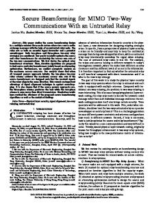
modeled as white Rn = σn2 I, where σn2 is the noise power. (For simulations with more realistic wireless multi-antenna channel models including spatial and frequency correlation, the reader is referred to [15, 16, 17].) The SNR is defined as SNR = PT /σn2 , which is essentially a measure of the transmitted power normalized with respect to the noise. In the first example, four different methods have been simulated by minimizing a cost function subject to a power constraint (recall that this is equivalent to minimizing the power subject to a global constraint as in §2.4.3): the classical minimization of the sum of the MSEs (SUM-MSE), the minimization of the product of the MSEs (PROD-MSE), the minimization of the maximum of the MSEs (MAX-MSE), and the minimization of the average/sum of the BERs (SUM-BER). The methods are evaluated in terms of BER averaged over the substreams; to be more precise, the outage BER13 (over different realizations of H) is considered since it is a more realistic measure than the average BER (which only makes sense when the system does not have delay constraints and the duration of the transmission is sufficiently long such that the fading statistics of the channel can be averaged out). In Figure 2.6, the BER (for a QPSK constellation) is plotted as a function of 13 The outage BER is the BER that is attained with some given probability (when it is not satisfied, an outage event is declared).
CONVEX OPTIMIZATION IN MIMO CHANNELS
31
Achievable Region of MSEs 0.05 Schur−convex SUM−MSE (Schur−concave) PROD−MSE (Schur−concave) 0.04
Pareto−optimal boundary
MSE2
0.03
0.02
0.01 Achievable Region
Non−achievable Region 0
0
0.01
0.02
0.03
0.04
0.05
MSE1
Figure 2.7: Achievable region of the MSEs for a given channel realization of a 4 × 4 MIMO channel with L = 2, along with the location of the design with the methods: PROD-MSE, SUM-MSE, and a Schur-convex (MAX-MSE and SUM-BER).
the SNR for a single 4 × 4 MIMO channel with L = 3 for the cases of ZF and MMSE receivers. It can be observed that the ZF receiver performs almost the same as the MMSE receiver thanks to the joint optimization of the transmitter and receiver (as opposed to the typically worse performance of the ZF receiver in the classical equalization setup where only the receiver is optimized). The methods MAX-MSE and SUM-BER correspond to Schur-convex functions and, as expected, are exactly the same (c.f. §2.4.3). The superiority of Schur-convex designs (MAX-MSE and SUMBER) with respect to Schur-concave designs (SUM-MSE and PROD-MSE) is very clear from Figure 2.6, as was argued in §2.4.3, due to the increase robustness against fading of the channel eigenmodes. In Figure 2.7, the achievable region in terms of MSEs is plotted for a given realization of a single 4 × 4 MIMO channel with L = 2 (MMSE receiver) and with an SNR of 15 dB. The achievable region has been computed with the method developed in §2.4.2 that allows to specify independent QoS constraints on each substream. The boundary between the achievable and non-achievable regions corresponds to the Pareto-optimal designs, characterized by not being outperformed by any other solution simultaneously in all substreams. The solutions corresponding to the previous methods, SUM-MSE, PROD-MSE, Schur-convex method (which includes MAX-MSE and SUM-BER), are also indicated. They clearly lie on the Pareto-optimal frontier,
CONVEX OPTIMIZATION IN MIMO CHANNELS
32
although in different points of it. In fact, since Schur-convex methods have equal MSEs on all substreams, they all correspond to the intersection of the Pareto-optimal boundary with the line ρ1 = ρ2 = · · · = ρL , which corresponds to a complete fairness among substreams.
2.5 2.5.1
An Application to Robust Transmitter Design in MIMO Channels Introduction and State of the Art
In §2.4, a general framework has been presented to jointly design optimum linear transmitters and receivers according to a set of optimization criteria based on convex optimization theory. In those cases, it has been assumed that a perfect channel estimate or CSI is available during the design stage. In a realistic scenario, however, the channel knowledge is generally imperfect. In such a situation, the design should take into account explicitly the errors in the channel estimate, leading to the so called robust designs, which are less sensitive to these errors. It is interesting to note that the first applications of robust designs were not for wireless communications, but for control theory (see [66, 67] and references therein). Indeed, the concepts of signal state space and MIMO were originally used in that area. Afterwards, all these techniques and concepts were extended to other fields due to their potential benefits. In some works such as [65, 68, 69, 70], the performance degradation of several non-robust designs for multi-antenna systems was analyzed, in which the errors in the CSI were considered negligible. The main conclusion is that this degradation increases rapidly with the error level. In a communication system, the receiver usually acquires the channel estimate using a training sequence (pilot symbols). At the transmitter, the CSI can be obtained through a feedback channel or from previous received signals, exploiting the channel reciprocity principle in a time division duplexing (TDD) system (see [36] for an overview of different channel estimation strategies). Different sources of errors in the CSI can be identified. In case of exploiting the channel reciprocity, the Gaussian noise from the estimation process and the outdated estimate due to the channel variability have to be considered. If a feedback channel is used, additional effects arise, such as the quantization of the channel estimate and the errors in the communication through the feedback channel. According to the way the error in the channel estimate is modeled, the robust techniques can be classified into two families: the Bayesian (or stochastic) and the maximin (or worst-case) approaches [14, 17]. In the Bayesian philosophy, the statistics of the error are assumed to be known and a stochastic measure of the system performance is optimized, such as the mean value. On the other hand, the maximin approach considers that the error belongs to a predefined uncertainty region and the final objective is the optimization of the worst system performance for any error in this region. The Bayesian philosophy has been considered in works such as [71], where a multiantenna transmitter was designed to maximize the mean SNR and the mutual in-
CONVEX OPTIMIZATION IN MIMO CHANNELS
33
formation assuming two sources of errors: the Gaussian noise and the quantization errors. The minimization of the BER was considered in [72]. Transmit FIR filters in a multi-antenna frequency-selective channel were designed in [73] to maximize the mean SNR and minimize the MSE assuming Gaussian errors. The more general case of MIMO flat fading channels was considered in [74], where the transmitter was composed of an orthogonal space-time block code (OSTBC) and a matrix performing a linear transformation. This matrix was designed to minimize an upper bound of the BER assuming Gaussian errors. A similar scheme consisting on the combination of an OSTBC a set of beamformers was considered in [75] to minimize the error probability. The same objective was taken in [76] and [77] for a MIMO frequency-selective channel using a multicarrier modulation: in [76], the transmitter and the receiver were based on matrices performing a linear transformation, whereas in [77], the transmitter was composed of an Alamouti’s code [11] combined with two beamformers. Regarding the maximin approach, [78] and [79] provide a general insight using a game theoretic formulation and describing several applications in signal processing. See also [18] for a reference on the theory of saddle-functions and maximin. This approach has been recently used in the classical problem of designing a receive beamformer under mismatches in the presumed model, as in [33], where the errors were assumed to be in the estimated steering vector and to belong to a spherical uncertainty region. This was afterwards generalized in [35] to embrace uncertainties both in the array response and the covariance matrix. The classical Capon’s beamformer [31] was extended to its robust version in [32], [34], and [80], taking generic uncertainty regions and different formulations. In some of these examples, the robustness was obtained by minimizing the output power of the beamformer while guaranteeing a minimum gain for any direction modeled by the uncertainty region (see §2.2.5 for a more detailed description). Finally, several applications of this robust approach to multiuser systems with multi-antenna base stations can also be found in [36], [81], and [82]. This subsection starts with the presentation of the generic formulation of the Bayesian and the maximin approaches in §2.5.2. Afterwards, a MIMO system is considered, where the robust transmitter is designed under the maximin philosophy and the receiver is based on an optimum ML detector assuming a perfect channel knowledge. This follows and extends the results obtained in [83].
2.5.2
A Generic Formulation of Robust Approaches
A generic formulation can be stated for both the Bayesian and the maximin approaches (see [17] for more details). In all the cases, the imperfect CSI can be represented as b +∆ H=H (2.69) b where H is the actual MIMO channel matrix (as defined in §2.3), H is the channel estimate, and ∆ is the error. The system performance is usually measured by a cost function f , whose minimization is the objective of the design (usual cost functions are based on the BER, the MSE, or the SINR, among others, c.f. §2.3.2). In the Bayesian approach, the error and the actual¡channel are¡modeled statisti¢ ¢ cally with the probability density functions (pdf’s) p∆ ∆ and pH H , respectively,
CONVEX OPTIMIZATION IN MIMO CHANNELS
34
which are assumed to be known. Note that knowing these pdf’s is equivalent to¡ know¢ b ing the pdf of the actual channel conditioned to the channel estimate pH|H b H|H , ¡ ¢ ¡ ¢ ¡ ¢ b pH H /p b H b by the Bayes rule. A possible design which is equal to p∆ H − H H strategy consists in the minimization of the mean value of the cost function f (note, however, that other stochastic measures of the performance could have been used, such as the outage performance). If this criterion is adopted and the average transmitted power is upper bounded by P0 , the following optimization problem has to be solved: £ ¡ ¢¤ EH|H minimize b f H, A, B A,B (2.70) ¡ ¢ subject to Tr BBH ≤ P0 where the optimization variables are the transmit B and the receive A matrices. Note that, in this case, although the average performance is optimized, no guarantee can be given in terms of the instantaneous performance. In the maximin approach, instead of modeling the error statistically, it is assumed that it belongs to a predefined uncertainty region R, i.e.,¡ ∆ ∈ R.¢ Then, the worst performance for any error in R is expressed as sup∆∈R f H, A, B . The robust design problem consists in the optimization of the worst performance, which can be formulated as ¡ ¢ sup f H, A, B minimize ∆∈R A,B (2.71) ¡ ¢ subject to Tr BBH ≤ P0 . In this case, a full statistical characterization is not necessary. Besides, this approach guarantees a minimum instantaneous performance for any error modeled by the uncertainty region, i.e., when the actual error behaves as expected (in a real situation, this will be satisfied with a high probability, declaring an outage otherwise). Note that this guarantee cannot be provided by the Bayesian approach optimizing the average performance.
2.5.3
Problem Formulation
As in §2.3 and §2.4, in the following, the transmission through a MIMO channel H is considered corresponding to the signal model y = Hs + n (see (2.23)). In particular, a multi-antenna flat fading wireless channel is assumed, where the number of transmit and receive antennas is nT and nR , respectively. The interference-plusnoise covariance matrix is Rn = σn2 I, corresponding to a scenario with only additive white Gaussian noise (AWGN). Note, however, that the derived design strategy can be applied to other kinds of MIMO channels as well. The objective is to obtain a maximin robust design of the system, as in (2.71), b at the transmitter as modeled in (2.69). according to an imperfect channel estimate H The CSI at the receiver will be assumed to be perfect. The Transmitter Architecture Consider that one symbol is to be transmitted at one time instant. From §2.4 it is concluded that, in the case of having a perfect CSI, the optimum solution is based on
CONVEX OPTIMIZATION IN MIMO CHANNELS
35
single beamforming (L = 1), consisting in the transmission through the eigenvector of HH H associated to the maximum eigenvalue (note that the squared whitened channel matrix is RH = σ12 HH H). In case that the channel knowledge is imperfect, n b HH b constitutes the naive or nontransmitting through the maximum eigenmode of H robust solution, which may be quite sensitive to the errors in the CSI. Therefore, a robust design is expected to use more eigenmodes than the maximum one. The design of the robust transmitter will be based on a linear processing, as in §2.3 (s = Bx), whereas at the receiver, a ML detector will be used assuming a perfect CSI. The direct design of a robust transmit matrix B seems very complicated and, therefore, a structure will be imposed on it to simplify the problem. The proposed robust solution consists in the transmission of the symbols through all the eigenmodes b using an adequate power distribution among them, as will be shown later b HH of H and as opposed to the non-robust design, where only the maximum eigenmode is used. Consider the simultaneous transmission of R independent complex symbols over Nt periods of time (leading to a transmission rate equal to R/Nt ), corresponding to the following linear signal model, similarly to linear dispersion codes [84] and OSTBC [85, 86, 87]: R ³ ´ X (r) (r) (i) (i) S= Bl xl + jBl xl ∈ CnT ×Nt (2.72) l=1
£ ¤ where xl is the lth transmitted complex symbol with a normalized energy (E |xl |2 = (r) (i) (r) (i) 1), xl and xl are its real and imaginary parts, respectively, Bl , Bl ∈ CnT ×Nt (r) (i) are the associated complex transmit matrices for xl and xl , and the rows of S are the Nt signal samples transmitted through each antenna. The structure imposed on the transmit matrices is ¡ ¢ ¡ ¢ (r) b diag {√pi } T(r) , B(i) = U b diag {√pi } T(i) Bl = U (2.73) l l l £ ¤ b = u b1 · · · u b nT ∈ CnT ×nT is the unitary matrix containing the nT eigenvecwhere U bi } sorted in decreasing order, pi is the power allocated b HH b with eigenvalues {λ tors of H (r) (i) to the ith estimated eigenmode, and Tl , Tl ∈ CnT ×Nt are matrices modeling a (r)
(r) H
(i)
(i) H
temporal spreading of the symbols and fulfilling Tl Tl = I and Tl Tl = I. (r) (i) These matrices Tl and Tl are based on the Hurwitz-Radon family of matrices (see [86] and [85]), so that the ML detector reduces to a bank of linear filters, and the detection scheme is the same as that used for OSTBC. This apparently complicated signaling scheme (2.72) can be represented as shown in Figure 2.8, where it is seen that the symbols are encoded by an OSTBC, and each output of the OSTBC is transmitted through a different estimated eigenmode. Finally, the parameters {pi } distribute the available power among the eigenmodes. This transmission scheme is similar to those presented in [74, 75, 88], among others, in which the transmitter architecture also consisted in the combination of an OSTBC and a beamforming stage, although the design of the power allocation was different to the one proposed in the following.
CONVEX OPTIMIZATION IN MIMO CHANNELS
36
power allocation beamforming
p1
...
...
u1
...
#1
...
pnT
u nT
...
...
OSTBC
...
R
{xl}l=1
# nT
Figure 2.8: General architecture for the transmitter based on the combination of an OSTBC block, a power allocation, and a beamforming stage.
Note that, in the signal model (2.72), not only the spatial, but also the temporal dimensions are exploited. This signal model can be rewritten using the generic matrixvector notation presented in §2.3 as follows. Let sn be the nth column of S representing the transmitted vector during the nth period of time. This vector can be expressed as (r) (i) sn = Bn xr + jBn xi (2.74) ¡ ¢ ¡ ¢ (r) b diag {√pi } T(r) and B(i) = U b diag {√pi } T(i) , the matrices T(r) where Bn = U n n n n (i)
(r)
(i)
and Tn contain the nth columns of Tl and Tl for l = 1, . . . , R, and xr = £ (r) £ (i) (r) ¤T (i) ¤T x1 · · · xR , xi = x1 · · · xR . The design objective is to calculate the optimum power allocation strategy {pi } subject to a transmit power constraint and adopting an adequate performance criterion. If the transmit power budget is P0 , the power constraint can be expressed in terms of the factors {pi } as n
T ¢ X 1 ¡ (r) 2 (i) kBl kF + kBl k2F = pi ≤ P0 , 2 i=1
pi ≥ 0.
(2.75)
Note that the set of feasible power distributions is convex, since all the constraints given above are linear. For the considered system ((2.72) and (2.73)) using an OSTBC with ML detection, the performance can be measured by the SNR expressed as (see [86] and [85]) SNR =
³ ´ 1 b H HH HU b diag(p) Tr U σn2
(2.76)
CONVEX OPTIMIZATION IN MIMO CHANNELS 37 £ ¤T where p = p1 · · · pnT . Based on this, the performance function f is defined as ³ ´ ¡ ¢ b H HH HU b diag(p) (2.77) f p, ∆ = Tr U ³ ´ ¡ ¢ ¡ ¢ bH H b +∆ H H b +∆ U b diag(p) , = Tr U (2.78) whose maximization is the objective of the design and where the error model (2.69) has been used. This function is linear in p and, therefore, concave; and convex-quadratic in the error ∆. Note that, in this case, an opposite strategy is taken from that presented in §2.4, in which the transmitted power was minimized subject to QoS constraints, although both kinds of problems are essentially equivalent, as explained in §2.4.1. The Maximin Problem Formulation As stated in §2.5.2, the maximin approach can be used to include robustness in the design. Accordingly, an uncertainty region R for ∆ has to be defined, which, in the following, will be assumed to be convex.14 The robust power distribution p? , which optimizes the worst performance for any error in the uncertainty region, can be found as the solution to the following optimization problem: ¡ ¢ inf f p, ∆ maximize ∆∈R p (2.79) subject to 1T p ≤ P0 pi ≥ 0 £ ¤T where 1 = 1 · · · 1 ∈ RnT ×1 is the all-one vector. The direct way to solve the maximin problem is to obtain the minimization of f with respect to ∆ in an analytical way and then solve the outer maximization. Such an approach, however, is difficult because it is not clear what is the minimizing ∆ for a given p in closed form. Of course, one can also consider solving the problem numerically, i.e., solving the inner minimization fe(p) = inf f (p, ∆) (2.80) ∆∈R
numerically for a given p, and then solving the outer maximization maxp fe(p) also numerically. Note that the inner minimization is a convex problem, since f is convex in ∆ and the constraint set R is also convex. The outer maximization is also a convex problem since the constraint set for p is convex and the function fe is concave. Consequently, the numerical algorithms referenced in §2.2.4 could be used. The proof that fe is concave is given below, where p1 and p2 are any feasible power distributions, 14 The
set R is convex if ∆ = θ∆1 + (1 − θ)∆2 ∈ R for any ∆1 , ∆2 ∈ R and θ ∈ [0, 1].
CONVEX OPTIMIZATION IN MIMO CHANNELS
38
and θ ∈ [0, 1]: fe(θp1 + (1 − θ)p2 ) = inf f (θp1 + (1 − θ)p2 , ∆) ∆∈R
= inf [θf (p1 , ∆) + (1 − θ)f (p2 , ∆)] ∆∈R
≥ θ inf f (p1 , ∆) + (1 − θ) inf f (p2 , ∆) ∆∈R
∆∈R
= θfe(p1 ) + (1 − θ)fe(p2 )
(2.81)
where the linearity of f in p has been used in the second equality. This numerical procedure guarantees that the desired solution p? is found, however, it is computationally costly because each iteration of the method for the outer maximization requires an evaluation of fe(p) (and possibly its gradient as well), which in turn requires solving the inner minimization numerically with as many iterations as needed to converge. Other kinds of numerical iterative methods could be used, such as the algorithm proposed in [89] to find saddle-points of maximin problems based on the method of steepest descent. In [90], an alternative algorithm for the same problem is derived based on the interior point approach.
2.5.4
Reformulating the Problem in a Simplified Convex Form
The objective is to rewrite the maximin problem (2.79), which is already convex but not amenable for efficient resolution, into an equivalent simplified convex problem so that it can be solved requiring less computational effort (see §2.2). The function f (p, ∆), which is concave-convex, and the optimization sets for the power distribution and the error satisfy the conditions given in Corollary 37.6.2 in [18]. From it, it can be concluded that there exists a saddle-point of the maximin problem, i.e., there exist p? and ∆? fulfilling the constraints and satisfying f (p, ∆? ) ≤ f (p? , ∆? ) ≤ f (p? , ∆)
(2.82)
for any feasible p and ∆. The solution to the original maximin problem (2.79) can be shown to be p? , and the saddle-value f ? , f (p? , ∆? ) is the minimum value of f given p? , i.e., fe(p? ) (see Lemma 36.2 in [18]). The existence of the saddle-point allows to rewrite the original maximin problem (2.79) using a minimax formulation, i.e., the inner and the outer optimizations can be interchanged: ¡ ¢ sup f p, ∆ minimize 1T p≤P0 ,pi ≥0 (2.83) ∆ subject to ∆ ∈ R, with the that the inner maximization is now very simple. In particular, ¡ advantage ¢ supp f p, ∆ gives as a result the maximum element of the diagonal of the matrix ¢ ¢ ¡ ¡ b multiplied by the power budget P0 , i.e.: b +∆ U b +∆ H H bH H U h ¢ i ¢ ¡ ¡ b b +∆ U b +∆ H H bH H (2.84) sup f (p, ∆) = P0 max U 1T p≤P0 ,pi ≥0
i
ii
n ¡ ¢ o ¢H ¡ b +∆ u b bi . bH H = P0 max u i H+∆ i
(2.85)
CONVEX OPTIMIZATION IN MIMO CHANNELS
39
Note that the power allocation p achieving this optimum value is not unique if the maximum value is attained by more than one element of the diagonal of the matrix ¡ ¢ ¡ ¢ b +∆ H H b + ∆ U. b bH H U As a consequence from the previous result, the original problem can now be written as the following simple convex minimization problem: minimize t,∆
subject to
t ¡ ¢H ¡ ¢ b b +∆ u bi bH H t ≥ P0 u i H+∆ ∆ ∈ R.
(2.86)
∀i
Solving the previous problem gives the saddle-value f ? = f (p? , ∆? ) = t? and the worst-case error ∆? of the saddle-point of the problem (see [18]); however, the optimal robust power distribution is still unknown. It turns out that the optimum Lagrange ¡ ¢H ¡ ¢ b b +∆ u bH b i in multipliers γi? associated with the constraints t ≥ P0 u H i H + ∆ problem (2.86) provide the optimum normalized power distribution p?i , i.e., p?i = P0 γi? , as proved below. The problem (2.86) can be solved by formulating the KKT conditions, which are satisfied by the worst-case error ∆? along with the optimum dual variables (see §2.2.3). On the other hand, it is clear that the worst-case error ∆? is also the solution to the problem inf ∆ (p? , ∆) (from (2.82)), where p? = arg maxp f (p, ∆? ) is the robust power distribution, and, therefore, the worst-case error ∆? must satisfy the KKT conditions for the problem inf ∆ f (p? , ∆). By a simple comparison of the KKT conditions for both problems, it is straightforward to see that for p?i = P0 γi? , the worst-case error ∆? satisfies both sets of KKT conditions and, hence, that is an optimal robust power allocation. The Lagrangian of the optimization problem (2.86) (characterizing for convenience and w.l.o.g. the uncertainty ¡ ¢convex region R as the intersection of a set of convex constraints of the form fi ∆ ≤ 0) is L1 = t + Ã
nT X
³ ´ X ¡ ¢H ¡ ¢ b b +∆ u bH bi − t + γi P0 u H µi fi (∆) i H+∆
i=1
=t 1−
nT X
! γi + P0 Tr
(2.87)
i
³¡ ´ X ¢ ¡ ¢ b +∆ H H b +∆ U b diag({γi })U bH + H µi fi (∆),
i=1
i
PnT b b H has been used. The KKT condibiu bH where the relation i=1 γi u i = U diag({γi })U tions for this problem are
nT X i=1
γi? = 1,
¢ ¢ ¡ ¡ ? H b b bi, bH H + ∆? u fi (∆? ) ≤ 0, t? ≥ P0 u i H+∆ ? ? µi ≥ 0, γi ≥ 0, X ¢ ¡ b diag({γ ? })U bH + b + ∆? U µ?i ∇fi (∆? ) = 0, P0 H i
(2.88) (2.89) (2.90)
i
´ ³ ¢ ¢ ¡ ¡ ? H b b b i − t? = 0. bH H + ∆? u µ?i fi (∆? ) = 0, γi? P0 u i H+∆
(2.91)
CONVEX OPTIMIZATION IN MIMO CHANNELS
40
On the other hand, the Lagrangian for the problem inf ∆ f (p? , ∆) is ³ ´ X ¡ ¢ ¡ ¢ bH H b +∆ H H b +∆ U b diag(p? ) + L2 = Tr U αi fi (∆)
(2.92)
i
and the KKT conditions for the optimal error and multipliers are: fi (∆? ) ≤ 0, αi? ≥ 0,
X ¡ ¢ b + ∆? U b diag(p? )U bH + H αi? ∇fi (∆? ) = 0,
(2.93) (2.94) (2.95)
i
αi? fi (∆? ) = 0.
(2.96)
From the comparison of both sets of KKT conditions (2.88)-(2.91) and (2.93)(2.96), it is clear that they are satisfied by the same worst-case error ∆? if αi? = µ?i and p?i = P0 γi? . Note that the transmit power constraints are automatically fulfilled, since the optimum dual variables {γi? } are required to satisfy γi? ≥ 0 (see (2.89)) and P nT ? i=1 γi = 1 (see (2.90)). It is important to remark that the saddle-value t? can be attained by more than ¡ ¢ ¡ ¢ bH H b + ∆? H H b + ∆? U. b Taking this one element of the diagonal of the matrix P0 U ¡ ¢ ¡ ¢ ¢ ¡ H ? ? H ? b +∆ b +∆ u b i − t? = 0 in bi H H into account, and using the condition γi P0 u (2.91), it is concluded that there can exist more than one Lagrange multipler γi? that can be different from zero; in other words, the robust power distribution can use more than one estimated eigenmode for transmission, as expected. This will be proved with some examples in the simulations section. Summarizing, the original maximin robust power allocation problem (2.79) can be solved by means of the simplified convex problem (2.86). The values of the optimum Lagrange multipliers of this simplified problem provide the normalized power distribution to be applied among the estimated eigenmodes. Currently, most of the existing software packages provide simultaneously the optimum values of both the primal and the dual variables and, therefore, they could be applied to find the optimum solution to this robustness problem (see §2.2.4 and references therein).
2.5.5
Convex Uncertainty Regions
The definition of the uncertainty region R may impact importantly on the system performance. The size and the shape of this region should take into account the quality of the channel estimate and the imperfections that generate the error (see §2.5.1 for some examples of sources of errors). In the following, two sources of errors are identified and three different uncertainty regions, jointly with their sizes, are described. In all the cases, the proposed uncertainty regions are convex, as required to solve the optimization problem. Estimation Gaussian Noise A common situation when estimating the channel corresponds to the presence of AWGN, especially in TDD systems, where the transmitter can estimate the channel
CONVEX OPTIMIZATION IN MIMO CHANNELS i
i
r
(a)
41 i
r
r
(b)
(c)
Figure regions for the case of a scalar error ∆, where ∆r = © ª2.9: Different uncertainty © ª Re ∆ and ∆i = Im ∆ . (a) estimation Gaussian noise, (b) quantization errors, and (c) combined estimation and quantization errors.
while receiving in the reverse link, and use it as an estimate in the forward link, due to the channel reciprocity principle. The following assumptions are considered: all the components of the actual channel H are i.i.d. and follow a zero-mean circularly symmetric Gaussian distribution with a variance equal to σh2 , whereas the estimation AWGN is also zero-mean and circularly symmetric with variance σe2 . Based on this, the estimation SNR, i.e., the received SNR during the transmission of the training sequence, is defined as SNRest = σh2 /σe2 . Under these assumptions, the actual channel H conditioned to the channel estimate follows a circulary symmetric complex Gaussian distribution with a mean value equal to the MMSE Bayesian channel estimate and a white covariance matrix with 2 σ2 σ2 σh diagonal elements equal to σ2h+σe2 = 1+SNR (see [55]), i.e., the actual channel can est e h be assumed to be in a region near the MMSE Bayesian channel estimate, where the 2 σh . Therefore, in this case, it is natural distance to it is measured indirectly by 1+SNR est b to identify H as the MMSE Bayesian estimate of the MIMO channel and√to define the b with a radius equal to ² as follows: uncertainty region R as a sphere centered at H © ª R = ∆ : k∆k2F ≤ ² . (2.97) Since the error ∆ is Gaussian distributed, it will be inside the region R with a certain probability Pin lower than 1. This probability will be equal to the probability of providing the required QoS to the user. The mathematical relationship between ¡ ¢ the size of the uncertainty region, measured by ², and Pin is given be ² = ϕ−1 Pin , where the function ϕ is the cumulative density function of the chi-square distribution corresponding to k∆k2F with 2nR nT degrees of freedom and normalized variance 2 σh 2+2SNRest .
CONVEX OPTIMIZATION IN MIMO CHANNELS
42
Quantization Errors In frequency division duplexing (FDD) systems, the estimate of the channel at the transmitter is typically obtained through a feedback channel from the receiver to the transmitter. Since this feedback is expected to be discrete, the channel estimate has to be quantized introducing an error in the CSI available at the transmitter. Assuming that the receiver has a perfect knowledge of the channel response H, let us consider, for illustrative purposes, that a suboptimum uniform quantization is applied to the real and imaginary parts of all the components of H using a quantization step equal to b In this situation, the quantization SNR is given by SNRq = 6σ 2 /∆2 . ∆q , obtaining H. q h b as Consequently, the uncertainty region can be defined as a cube centered at H ½ ¾ ¯ © ª¯ ∆q ¯ © ª¯ ∆q ¯ ¯ ¯ ¯ R = ∆ : Re [∆]ij ≤ , Im [∆]ij ≤ . (2.98) 2 2 As the capacity of the feedback channel increases, more bits can be used in the quantization and, therefore, the size of the uncertainty region can be reduced. Combined Estimation and Quantization Errors In a realistic scenario with feedback, the two effects considered previously, i.e., the presence of AWGN and the quantization errors, are expected to be combined. This can be modeled mathematically by defining an appropriate uncertainty region as ½ ¾ 2 ∆ = ∆1 + ∆2 : k∆ ¯ 1©kF ≤ ²,ª¯ ∆q ¯ © ª¯ ∆q , R= (2.99) ¯Re [∆2 ]ij ¯ ≤ ¯ ¯≤ 2 , Im [∆2 ]ij 2 which is convex because it is described by linear and norm constraints [14]. With this region, the optimization problem (2.86) can be rewritten as the following quadratic convex minimization problem: minimize t,∆1 ,∆2
subject to
t ¡ ¢ ¡ ¢ b + ∆1 + ∆2 H H b + ∆1 + ∆2 u bi bH t ≥¡ P0 u i H ¢ H Tr ∆ ∆ ≤ ² 1 1 ¯ © ¯ © ª¯ ª¯ ¯Re [∆2 ]ij ¯ ≤ ∆q , ¯Im [∆2 ]ij ¯ ≤ ∆q , 2
∀i
(2.100)
2
which comprises the previous uncertainty regions and the corresponding optimization problems as particular cases. Figure 2.9 illustrates the shape of the three considered uncertainty for the © ª © regions ª concrete case of a scalar error ∆, where ∆r = Re ∆ and ∆i = Im ∆ .
2.5.6
Numerical Results
This section provides some numerical results to illustrate the performance of the proposed robust design when compared to other known transmission techniques. The robust design takes into account the uncertainty in the channel knowledge to find an optimum power distribution among the estimated eigenmodes. When the
CONVEX OPTIMIZATION IN MIMO CHANNELS
43
g=1 g = 0.75 g = 0.5 g = 0.25
H H
F
Figure 2.10 Spherical uncertainty regions for different values of the parameter g.
channel estimate is perfect, the robust solution must lead to the same power distribution as for the non-robust beamforming. As stated in §2.5.3, the non-robust design consists in transmitting all the symbols only through the maximum estimated eigenmode, which can be formulated in terms of the power distribution as p1 = P0 , pi = 0, i = 2, . . . , nT , i.e., all the power is allocated to the maximum eigenmode. When the channel uncertainty increases, the robust design tends to distribute the power in a more uniform way, increasing the power for the weaker eigenmodes. In the first example, a system with 4 transmit and√6 receive antennas is studied. b F , 0 < g ≤ 1 are Spherical uncertainty regions with a radius equal to ² = gkHk b + ∆ 6= 0, ∀∆ ∈ R. This considered. Note that for these uncertainty regions, H = H condition is imposed since, otherwise, the saddle-value would be equal to 0. In Figure 2.10, the spherical uncertainty regions for different sizes are represented. Since nT = 4, the total transmitted power has to be distributed among the 4 estimated eigenmodes. Figure 2.11 shows the mean value of the normalized robust power distribution given by {γi? }, that is, assuming P0 = 1. As it is seen, for g = 0 the power distribution corresponds to the non-robust approach, as expected. As g increases, the errors in the channel estimate are higher and the power allocation profile changes so that the power is distributed in a more uniform way. Figures 2.12 and 2.13 show some simulations results in order to compare three different techniques: the proposed maximin robust approach, the non-robust technique, and a pure OSTBC in which no CSI is available at the transmitter. The techniques are compared in terms of the minimum required transmitted power so that the resulting SNR is higher than a target SNR0 = 10 dB for any error in the uncertainty
CONVEX OPTIMIZATION IN MIMO CHANNELS
44
Mean Value of the Normalized Power Allocation 1 Mean value of γ 1 Mean value of γ 2 Mean value of γ 3 Mean value of γ4
0.9
0.8
0.7
Mean Value of γi
0.6
0.5
0.4
0.3
0.2
0.1
0
0
0.1
0.2
0.3
0.4
0.5 0.6 Parameter g
0.7
0.8
0.9
1
Figure 2.11: Mean value of the normalized robust power distribution for different sizes of the uncertainty regions.
region. These results are given as a function of the estimation and the quantization SNR. In Figure 2.12, a TDD system has been considered with Gaussian estimation noise and assuming spherical uncertainty regions. The number of antennas is nT = 2, nR = 2 and, therefore, the transmission rate is 1. Two different probabilities of providing the required QoS have been considered: Pin = 0.6 and Pin = 0.85. As Pin increases, more power is necessary since the uncertainty region grows in order to guarantee the required performance with a higher probability. Besides, as the estimation SNR increases, less power is necessary, since the quality of the CSI improves. An interesting conclusion obtained from the figure is that, if the estimation SNR is high enough, the OSTBC technique needs more power than the non-robust and the robust solutions, since it does not exploit the channel knowledge. On the contrary, if the estimation SNR is low enough, the non-robust solution may need more power than OSTBC, concluding that in case that the CSI has a very low quality, it is not convenient to exploit that knowledge, unless using the robust solution. Note that, for all the estimation SNR range, the robust technique is the one requiring less power. Very similar conclusions can be obtained from Figure 2.13 in terms of the quantization SNR. Once again, the robust technique needs less transmitted power than
CONVEX OPTIMIZATION IN MIMO CHANNELS
45
Mean value of the Minimum Transmitted Power (dB) − TDD System − Spherical Uncertainty Regions Non−Robust. Pin=0.85. nT=2, nR=2 OSTBC. Pin=0.85. nT=2, nR=2 Robust. Pin=0.85. nT=2, nR=2 Robust. Pin=0.6. nT=2, nR=2
Mean value of the Minimum Transmitted Power (dB)
22
20
18
16
14
12
10 8
9
10
11 Estimation SNR (dB)
12
13
14
Figure 2.12: Minimum transmitted power in a TDD system assuming spherical uncertainty regions.
the other ones to fulfill the performance requirements represented by SNR0 = 10 dB. In the same figure, the performance is also compared for two different antennas configurations: nT = 4, nR = 4 (rate 3/4) and nT = 6, nR = 6 (rate 1/2). From the simulations it is concluded that, as expected, increasing the number of antennas implies a reduction in the required transmitted power.
2.6
Summary
This chapter has given an overview of convex optimization theory with emphasis on the art of unveiling the hidden convexity of engineering problems and then has considered the design of linear MIMO transceivers or beamforming under the powerful framework of convex optimization theory. The design of linear MIMO transceivers is a complicate nonconvex problem with matrix-valued variables. After several manipulations, the problem has been reformulated as a simple convex problem with scalar-valued variables. Then, the theory of convex optimization has been used to derive simple and efficient algorithms to compute the achievable region and, in particular, closed-form solutions have been obtained for the family of Schur-concave/convex functions such as the minimization
REFERENCES
46
Mean value of the Minimum Transmitted Power (dB) − FDD System − Cubic Uncertainty Regions 11 Non−Robust. n =4, n =4 T R OSTBC. n =4, n =4 T R Robust. n =4, n =4 T R Non−Robust. nT=6, nR=6 OSTBC. nT=6, nR=6 Robust. nT=6, nR=6
Mean value of the Minimum Transmitted Power (dB)
10
9
8
7
6
5
4
3
2
1
5
6
7
8
9 10 Quantization SNR (dB)
11
12
13
14
Figure 2.13: Minimum transmitted power in a FDD system assuming cubic uncertainty regions.
of the average BER of the system. Finally, a robust transmission scheme for MIMO channels has been proposed based on the combination of an OSTBC, a power allocation, and a beamforming stage. The design of the power allocation is performed according to an imperfect channel estimate under the maximin philosophy, by which the worst performance is optimized for any error in the channel estimate described by an uncertainty region. The original maximin optimization problem corresponding to the design of the robust power allocation, which consists of two stages (inner and outer optimizations), is first formulated and then is transformed into a simple single-stage convex optimization problem, whose optimal Lagrange multipliers provide the optimum power allocation. For several examples of uncertainty regions, this optimization problem is shown to reduce to a convex quadratic problem.
References [1] G. J. Foschini, “Layered space-time architecture for wireless communication in a fading environment when using multi-element antennas,” Bell Labs Technical Journal, vol. 1, no. 2, pp. 41–59, Autumn 1996.
REFERENCES
47
[2] G. G. Raleigh and J. M. Cioffi, “Spatio-temporal coding for wireless communication,” IEEE Trans. Commun., vol. 46, no. 3, pp. 357–366, March 1998. [3] I. E. Telatar, “Capacity of multi-antenna Gaussian channels,” European Trans. Telecommun., vol. 10, no. 6, pp. 585–595, Nov.-Dec. 1999. [4] G. Foschini and M. Gans, “On limits of wireless communications in a fading environment when using multiple antennas,” Wireless Personal Communications, vol. 6, pp. 311–335, 1998. [5] M. L. Honig, K. Steiglitz, and B. Gopinath, “Multichannel signal processing for data communications in the presence of crosstalk,” IEEE Trans. Commun., vol. 38, no. 4, pp. 551–558, April 1990. [6] A. Scaglione, G. B. Giannakis, and S. Barbarossa, “Redundant filterbank precoders and equalizers Part I: Unification and optimal designs,” IEEE Trans. Signal Processing, vol. 47, no. 7, pp. 1988–2006, July 1999. [7] H. B¨ olcskei and A. J. Paulraj, “Multiple-input multiple-output (MIMO) wireless systems,” in The Communications Handbook, 2nd ed., pp. 90.1–90.14, J. Gibson, Ed. CRC Press, 2002. [8] K. Miettinen, Multi-Objective Optimization. Kluwer Academic Publishers, 1999. [9] C. E. Shannon, “A mathematical theory of communication,” The Bell System Technical Journal, vol. 27, pp. 379–423, 623–656, July-Oct. 1948. [10] T. M. Cover and J. A. Thomas, Elements of Information Theory. New York: Wiley, 1991. [11] S. M. Alamouti, “A simple transmit diversity technique for wireless communications,” IEEE J. Select. Areas Commun., vol. 16, no. 8, pp. 1451–1458, Oct. 1998. [12] V. Tarokh, N. Seshadri, and A. R. Calderbank, “Space-time codes for high data rate wireless communications: Performance criterion and code construction,” IEEE Trans. Inform. Theory, vol. 44, no. 2, pp. 744–765, March 1998. [13] D. P. Bertsekas, Nonlinear Programming, 2nd ed. Belmont, Massachusetts: Athena Scientific, 1999. [14] S. Boyd and L. Vandenberghe, Convex Optimization. Cambridge University Press, 2004. [15] D. P. Palomar, J. M. Cioffi, and M. A. Lagunas, “Joint Tx-Rx beamforming design for multicarrier MIMO channels: A unified framework for convex optimization,” IEEE Trans. Signal Processing, vol. 51, no. 9, pp. 2381–2401, Sept. 2003. [16] D. P. Palomar, M. A. Lagunas, and J. M. Cioffi, “Optimum linear joint transmit-receive processing for MIMO channels with QoS constraints,” IEEE Trans. Signal Processing, vol. 52, no. 5, pp. 1179–1197, May 2004. [17] D. P. Palomar, “A unified framework for communications through MIMO channels,” Ph.D. dissertation, Technical University of Catalonia (UPC), Barcelona, Spain, May 2003. [18] R. T. Rockafellar, Convex Analysis, 2nd ed. Princeton, NJ: Princeton Univ. Press, 1970. [19] D. G. Luenberger, Optimization by Vector Space Methods. New York: Wiley, 1969. [20] R. T. Rockafellar, “Lagrange multipliers and optimality,” SIAM Review, vol. 35, no. 2, pp. 183–238, 1993. [21] M. S. Lobo, L. Vandenberghe, S. Boyd, and H. Lebret, “Applications of second-order cone programming,” Linear Algebra and Applications, vol. 284, no. 1-3, pp. 193–228, July 1998.
REFERENCES
48
[22] L. Vandenberghe and S. Boyd, “Semidefinite programming,” SIAM Review, vol. 38, no. 1, pp. 49–95, March 1996. [23] A. Ben-Tal and A. Nemirovski, Lectures on Modern Convex Optimization: Analysis, Algorithms, and Engineering Applications. Society for Industrial and Applied Mathematics, 2001. [24] Y. Nesterov and A. Nemirovski, “Interior-point polynomial methods in convex programming,” SIAM Studies in Applied Mathematics, vol. 13, 1994. [25] J. F. Sturm, “Using sedumi 1.02, a MATLAB toolbox for optimization over symmetric cones,” Optimization Methods and Software, vol. 11-12, pp. 625–653, 1999. [26] J.-L. Goffin and J.-P. Vial, “Convex nondifferentiable optimization: A survey focussed on the analytic center cutting plane method,” Department of Management Studies, University of Geneva, Switzerland, Tech. Rep., Feb. 1999. [27] Z.-Q. Luo, “Applications of convex optimization in signal processing and digital communication,” Mathematical Programming, Series B, vol. 97, no. 1-2, pp. 177–207, July 2003. [28] H. Lebret and S. Boyd, “Antenna array pattern synthesis via convex optimization,” IEEE Trans. Signal Processing, vol. 45, no. 3, pp. 526–532, March 1997. [29] S.-P. Wu, S. Boyd, and L. Vandenberghe, “FIR filter design via spectral factorization and convex optimization,” in Applied and Computational Control, Signals and Circuits, vol. 1, ch. 5, pp. 215–245, B. Datta, Ed. Boston, MA: Birkhauser, 1999. [30] T. N. Davidson, Z.-Q. Luo, and J. F. Sturm, “Linear matrix inequality formulation of spectral mask constraints with applications to FIR filter design,” IEEE Trans. Signal Processing, vol. 50, no. 11, pp. 2702–2715, Nov. 2002. [31] R. A. Monzingo and T. W. Miller, Introduction to Adaptive Arrays. New York: Wiley, 1980. [32] R. Lorenz and S. P. Boyd, “Robust minimum variance beamforming,” IEEE Trans. Signal Processing, to appear 2004. [33] S. A. Vorobyov, A. B. Gershman, and Z.-Q. Luo, “Robust adaptive beamforming using worst-case performance optimization: A solution to the signal mismatch problem,” IEEE Trans. Signal Processing, vol. 51, no. 2, pp. 313–324, Feb. 2003. [34] J. Li, P. Stoica, and Z. Wang, “On robust Capon beamforming and diagonal loading,” IEEE Trans. Signal Processing, vol. 51, no. 7, pp. 1702–1715, July 2003. [35] S. Shahbazpanahi, A. B. Gershman, Z.-Q. Luo, and K. M. Wong, “Robust adaptive beamforming for general-rank signal models,” IEEE Trans. Signal Processing, vol. 51, no. 9, pp. 2257–2269, Sept. 2003. [36] M. Bengtsson and B. Ottersten, “Optimal and suboptimal transmit beamforming,” in Handbook of Antennas in Wireless Communications, L. C. Godara, Ed. Boca Raton, FL: CRC Press, 2001. [37] C. E. Shannon, “Coding theorems for a discrete source with a fidelity criterion,” IRE Nat. Conv. Rec., pp. 142–163, March 1959. [38] M. Chiang and S. Boyd, “Geometric programming duals of channel capacity and rate distortion,” IEEE Trans. Inform. Theory, vol. 50, no. 2, pp. 245–258, Feb. 2004. [39] L. Xiao, M. Johansson, and S. Boyd, “Simultaneous routing and resource allocation via dual decomposition,” IEEE Trans. Commun., vol. 52, no. 7, pp. 1136–1144, July 2004. [40] S. H. Low, L. L. Perterson, and L. Wang, “Understanding vegas: A duality model,” Journal of the ACM, vol. 49, no. 2, pp. 207–235, March 2002.
REFERENCES
49
[41] M. Chiang, “To layer or not to layer: balancing transport and physical layers in wireless multihop networks,” in Proc. IEEE INFOCOM, Hong Kong, China, March 2004. [42] W. Yu, W. Rhee, S. Boyd, and J. M. Cioffi, “Iterative water-filling for Gaussian vector multiple-access channels,” IEEE Trans. Inform. Theory, vol. 50, no. 1, pp. 145–152, Jan. 2004. [43] D. P. Bertsekas and J. N. Tsitsiklis, Parallel and Distributed Computation: Numerical Methods. Prentice Hall, 1989. [44] A. W. Marshall and I. Olkin, Inequalities: Theory of Majorization and Its Applications. New York: Academic Press, 1979. [45] Z.-Q. Luo, T. N. Davidson, G. B. Giannakis, and K. M. Wong, “Tranceiver optimization for block-based multiple access through ISI channels,” IEEE Trans. Signal Processing, vol. 52, no. 4, pp. 1037–1052, April 2004. [46] F. D. Neeser and J. L. Massey, “Proper complex random processes with applications to information theory,” IEEE Trans. Inform. Theory, vol. 39, no. 4, pp. 1293–1302, July 1993. [47] B. Picinbono, “On circularity,” IEEE Trans. Signal Processing, vol. 42, no. 12, pp. 3473–3482, Dec. 1994. [48] B. Picinbono and P. Chevalier, “Widely linear estimation with complex data,” IEEE Trans. Signal Processing, vol. 43, no. 8, pp. 2030–2033, Aug. 1995. [49] P. J. Schreier and L. L. Scharf, “Second-order analysis of improper complex random vectors and processes,” IEEE Trans. Signal Processing, vol. 51, no. 3, pp. 714–725, March 2003. [50] S. Benedetto and E. Biglieri, Principles of Digital Transmission: With Wireless Applications. New York: Kluwer Academic, 1999. [51] S. Verd´ u, Multiuser Detection. New York: Cambridge University Press, 1998. [52] K. Cho and D. Yoon, “On the general BER expression of one- and two-dimensional amplitude modulations,” IEEE Trans. Commun., vol. 50, no. 7, pp. 1074–1080, July 2002. [53] H. V. Poor and S. Verd´ u, “Probability of error in MMSE multiuser detection,” IEEE Trans. Inform. Theory, vol. 43, no. 3, pp. 858–871, May 1997. [54] D. P. Palomar, M. Bengtsson, and B. Ottersten, “Minimum BER linear transceivers for MIMO channels via primal decomposition,” accepted in IEEE Trans. Signal Processing, to appear 2005. [55] S. M. Kay, Fundamentals of Statistical Signal Processing: Estimation Theory. Englewood Cliffs, NJ: Prentice Hall, 1993. [56] K. H. Lee and D. P. Petersen, “Optimal linear coding for vector channels,” IEEE Trans. Commun., vol. COM-24, no. 12, pp. 1283–1290, Dec. 1976. [57] J. Salz, “Digital transmission over cross-coupled linear channels,” At&T Technical Journal, vol. 64, no. 6, pp. 1147–1159, July-Aug. 1985. [58] J. Yang and S. Roy, “On joint transmitter and receiver optimization for multiple-inputmultiple-output (MIMO) transmission systems,” IEEE Trans. Commun., vol. 42, no. 12, pp. 3221–3231, Dec. 1994. [59] H. Sampath, P. Stoica, and A. Paulraj, “Generalized linear precoder and decoder design for MIMO channels using the weighted MMSE criterion,” IEEE Trans. Commun., vol. 49, no. 12, pp. 2198–2206, Dec. 2001. [60] J. Yang and S. Roy, “Joint transmitter-receiver optimization for multi-input multioutput systems with decision feedback,” IEEE Trans. Inform. Theory, vol. 40, no. 5, pp. 1334–1347, Sept. 1994.
REFERENCES
50
[61] E. N. Onggosanusi, A. M. Sayeed, and B. D. V. Veen, “Efficient signaling schemes for wideban space-time wireless channels using channel state information,” IEEE Trans. Veh. Technol., vol. 52, no. 1, pp. 1–13, Jan. 2003. [62] Y. Ding, T. N. Davidson, Z.-Q. Luo, and K. M. Wong, “Minimum BER block precoders for zero-forcing equalization,” IEEE Trans. Signal Processing, vol. 51, no. 9, pp. 2410– 2423, Sept. 2003. [63] J. M. Cioffi, G. P. Dudevoir, M. V. Eyuboglu, and G. D. Forney, “MMSE decisionfeedback equalizers and coding - Parts I-II: Equalization results and coding results,” IEEE Trans. Commun., vol. 43, no. 10, pp. 2582–2604, Oct. 1995. [64] P. Viswanath and V. Anantharam, “Optimal sequences and sum capacity of synchronous CDMA systems,” IEEE Trans. Inform. Theory, vol. 45, no. 6, pp. 1984–1991, Sept. 1999. [65] A. Pascual-Iserte, A. I. P´erez-Neira, and M. A. Lagunas, “On power allocation strategies for maximum signal to noise and interference ratio in an OFDM-MIMO system,” IEEE Trans. Wireless Commun., vol. 3, no. 3, pp. 808–820, May 2004. [66] K. Zhou, J. C. Doyle, and K. Glover, Robust and Optimal Control. Upper Saddle River, NJ: Prentice-Hall, 1996. [67] B. Hassibi, A. H. Sayed, and T. Kailath, Indefinite Quadratic Estimation and Control: A Unified Approach to H2 and H∞ Theories. Philadelphia, PA: SIAM, 1999. [68] S. Zhou and G. B. Giannakis, “How accurate channel prediction needs to be for transmit-beamforming with adaptive modulation over Rayleigh MIMO channels?” IEEE Trans. Wireless Commun., vol. 3, no. 4, pp. 1285–1294, July 2004. [69] J. Choi, “Performance analysis for transmit antenna diversity with/without channel information,” IEEE Trans. Veh. Technol., vol. 51, no. 1, pp. 101–113, January 2002. [70] ——, “Performance limitation of closed-loop transmit antenna diversity over fast rayleigh fading channels,” IEEE Trans. Veh. Technol., vol. 51, no. 4, pp. 771–775, July 2002. [71] A. Narula, M. J. Lopez, M. D. Trot, and G. W. Wornell, “Efficient use of side information in multiple-antenna data transmission over fading channels,” IEEE J. Select. Areas Commun., vol. 16, no. 8, pp. 1423–1436, October 1998. [72] A. Wittneben, “Optimal predictive TX combining diversity in correlated fading for microcellular mobile radio applications,” in Proc. IEEE Global Telecommunications Conference (GLOBECOM 1995), pp. 13–17, Nov. 1995. [73] A. Pascual-Iserte, A. I. P´erez-Neira, and M. A. Lagunas, “Exploiting transmission spatial diversity in frequency selective systems with feedback channel,” in Proc. IEEE International Conference on Acoustics, Speech, and Signal Processing (ICASSP 2003), vol. 4, pp. 85–88, April 2003. [74] G. J¨ ongren, M. Skoglund, and B. Ottersen, “Combining beamforming and orthogonal space-time block coding,” IEEE Trans. Inform. Theory, vol. 48, no. 3, pp. 611–627, March 2002. [75] S. Zhou and G. B. Giannakis, “Optimal transmitter eigen-beamforming and space-time block coding based on channel mean feedback,” IEEE Trans. Signal Processing, vol. 50, no. 10, pp. 2599–2613, October 2002. azquez, “Transmit filter optimization based on partial [76] F. Rey, M. Lamarca, and G. V´ CSI knowledge for wireless applications,” in Proc. IEEE 2003 International Conference on Communications (ICC 2003), vol. 4, pp. 2567 –2571, Anchorage, AK, May 11-15, 2003.
REFERENCES
51
[77] P. Xia, S. Zhou, and G. B. Giannakis, “Adaptive MIMO-OFDM based on partial channel state information,” IEEE Trans. Signal Processing, vol. 52, no. 1, pp. 202–213, January 2004. [78] S. A. Kassam and H. V. Poor, “Robust techniques for signal processing: A survey,” Proceedings of the IEEE, vol. 73, no. 3, pp. 433–481, March 1985. [79] S. Verd´ u and V. Poor, “On minimax robustness: A general approach and applications,” IEEE Trans. Inform. Theory, vol. 30, no. 2, pp. 328–340, March 1984. [80] P. Stoica, Z. Wang, and J. Li, “Robust Capon beamforming,” IEEE Signal Processing Lett., vol. 10, no. 6, pp. 172–175, June 2003. [81] M. Bengtsson and B. Ottersten, “Optimal downlink beamforming using semidefinite optimization,” in Proc. 37th Annual Allerton Conference on Communications, Control, and Computing, pp. 987–996, Sept. 1999. [82] M. Biguesh, S. Shahbazpanahi, and A. B. Gershman, “Robust power adjustment for transmit beamforming in cellular communications systems,” in Proc. IEEE International Conference on Acoustics, Speech, and Signal Processing (ICASSP 2003), vol. 5, pp. 105–108, April 2003. [83] A. Pascual-Iserte, A. I. P´erez-Neira, and M. A. Lagunas, “A maximin approach for robust MIMO design: Combining OSTBC and beamforming with minimum transmission power requirements,” in Proc. IEEE International Conference on Acoustics, Speech, and Signal Processing (ICASSP 2004), vol. 2, pp. 1–4, May 2004. [84] B. Hassibi and B. M. Hochwald, “High-rate codes that are linear in space and time,” IEEE Trans. Inform. Theory, vol. 48, no. 7, pp. 1804–1824, July 2002. [85] G. Ganesan and P. Stoica, “Space-time block codes: A maximum SNR approach,” IEEE Trans. Inform. Theory, vol. 47, no. 4, pp. 1650–1656, May 2001. [86] V. Tarokh, H. Jafharkani, and A. R. Calderbank, “Space-time block codes from orthogonal designs,” IEEE Trans. Inform. Theory, vol. 45, no. 5, pp. 1456–1467, July 1999. [87] E. G. Larsson and P. Stoica, Space-Time Block Coding for Wireless Communications. Cambridge University Press, 2003. [88] S. Zhou and G. B. Giannakis, “Optimal transmitter eigen-beamforming and space-time block coding based on channel correlations,” IEEE Trans. Inform. Theory, vol. 49, no. 7, pp. 1673–1690, July 2003. [89] R. T. Rockafellar, “Saddle-points and convex analysis,” in Differential Games and Related Topics, pp. 109–127, H. W. Kuhn and G. P. Szego, Eds. North-Holland Publ. Co., 1971. ˇ [90] S. Zakovi´ c and C. Pantelides, “An interior point method algorithm for computing saddle points of constrained continuous minimax,” Annals of Operations Research, vol. 99, pp. 59–77, December 2000.