Spino¤s and the Market for Ideas Satyajit Chatterjee
Esteban Rossi-Hansberg
Federal Reserve Bank of Philadelphia
Princeton University
September 2010
Abstract We present a theory of entry through spino¤s in which workers generate productive ideas and possess private information concerning their quality. Because quality is privately observed, by the standard adverse-selection logic, the market can at best o¤er a price that re‡ects the average quality of ideas sold. This gives the holders of above-average-quality ideas the incentive to spin o¤. We show that only workers with very good ideas decide to spin o¤, while workers with mediocre ideas sell them. Entrepreneurs of existing …rms pay a price for the ideas sold in the market that implies zero expected pro…ts for them. Hence, …rms’ project selection is independent of …rm size, which, under some additional assumptions, leads to scale-independent growth. The entry and growth process of …rms leads to invariant …rm-size distributions that resemble the ones for the US economy and most of its individual industries.
1
Introduction
The generation and implementation of new ideas shapes industry dynamics and the structure of …rms. Ideas can be generated in many di¤erent contexts, but many important innovations have been developed by workers of established …rms. In some cases, workers sell their ideas to established …rms We thank Hal Cole, Ken Hendricks, Hugo Hopenhayn, Boyan Jovanovic, Chris Phelan, Victor Rios-Rull and participants at several seminars and conferences for useful comments. Rossi-Hansberg thanks the Sloan Foundation for …nancial support. The views expressed in this paper are those of the authors and do not necessarily re‡ect the views of the Federal Reserve System or the Federal Reserve Bank of Philadelphia. This paper is available free of charge at www.philadelphiafed.org/research-and-data/publications/working-papers/.
1
(including their own), and in other cases, they use them to start new …rms: spino¤s. Whether an innovation by a worker is implemented by existing …rms, leads to a spino¤, or is discarded depends on the initial knowledge about the idea, as well as the pro…ts that the di¤erent entities can generate by implementing it. In this paper, we present a theory of entry through spino¤s in which the key ingredient is the originator’s private information concerning the quality of his new idea. Because quality is privately observed, by the standard adverse-selection logic, the market can at best o¤er a price that re‡ects the average quality of ideas sold. This gives the holders of above-average-quality ideas the incentive to spin o¤. But spinning o¤ is costly and there is a critical quality level at which the loss from selling the idea at the market price balances the costs imposed by spinning o¤. Ideas that are of higher quality than this critical level lead to spino¤s, while ideas that are of lower quality than the critical level are sold to existing …rms. Our theory of spino¤s implies a new model of …rm entry and …rm growth. Ideas that are spun o¤ generate entry of new businesses, while ideas that are sold to existing …rms generate new employment in existing …rms. We take the view that when a person sets up his or her own business, the person has some new business idea in mind — it could be something as simple as a pizza store in a new location or something sophisticated like new business software. Our model of spino¤s encompasses both cases because the pizza store owner could have ‘sold’his idea of a new location to a national franchise by partnering with it and the owner of the new business software could have sold his invention to an existing software company. Thus, in a broad sense, entry occurs when these options to sell new ideas are not exercised, and growth of existing …rms occurs when they are exercised. This view also explains our terminology: we call our model a theory of spino¤s precisely because the alternative is to sell the new idea to an established …rm. We explore this model of entry and …rm growth at some length in the paper. There are several key elements in our theory. The …rst key element, of course, is private information. Speci…cally, we assume that a worker with a new idea has private information on the mean payo¤ from the idea. The worker can either decide to create a new …rm to implement the idea or sell the idea to an established …rm at a price that is independent of the (privately observed) mean return. If he does the latter, he can credibly reveal the mean return to the buying …rm after the sale, since there is nothing at stake for him at that point. Knowing the mean return, the buying …rm then decides whether to implement the idea. Low quality ideas are discarded without being implemented. Implementing an idea means producing with it for one period. Producing with an idea –either in a spino¤ or in an established …rm –reveals the actual payo¤ from the idea. We call an idea that has been implemented, and therefore that has a known payo¤, a project. Production
2
requires one unit of labor. Since labor is costly, the project payo¤ can be low enough to make further use non-optimal. In that case, the project is dropped. If the project payo¤ is su¢ ciently high, the project is run forever and provides a constant source of pro…ts to the entrepreneur who implemented it. The second key element is the costs of spinning o¤. We assume that managing one or more projects is a full-time job that leaves the entrepreneur no time to devote to inventing new ideas. Thus, becoming an entrepreneur implies giving up on the possibility of spinning o¤ in the future with an even better idea. Clearly this option to spin o¤ in the future has value and, consequently, prospective entrepreneurs – workers who decide to test an idea on their own – are more choosy about which projects to accept and run than established entrepreneurs. Because project returns are speci…c to the entrepreneur who tests the idea, projects that are discarded by a prospective entrepreneur cannot be sold to established entrepreneurs. This speci…city makes workers with ideas more selective in choosing which ideas to test on their own compared to established entrepreneurs. Thus the mean return at which established entrepreneurs are just willing to test an idea is lower than the mean return that just induces a worker to spin o¤ and test on his own. The gap in these thresholds implies that ideas can sell at a positive price in the market. To use an analogy, it is like having a ‘lemons problem’in which withholding a used car from the market is costly (because, say, the person has to pay insurance costs, garage fees, etc.) and, therefore, the person may sell a car even if the price fetched in the market is lower than the (privately observed) value of the car.1 The third key element is competition in the market for ideas. When individuals are risk neutral or have constant absolute risk aversion, and competition forces all the (expected) surplus from new ideas to go to the seller of the idea, the mean return for which established entrepreneurs are indi¤erent between testing an idea or discarding it is independent of the size of the entrepreneur’s …rm. Hence, in equilibrium, heterogenous …rms are indi¤erent about how many ideas to buy. If they …nd out about ideas at a rate proportional to their size, this implies scale-independent growth for established …rms, for which there is some evidence in the US data. If the market for ideas was not competitive, …rms would not be indi¤erent about the number of ideas they buy, and scaleindependent growth would not be an equilibrium outcome of the model. We show that this growth process, together with the entry process predicted by the model, leads to a realistic size distribution 1 It seems plausible that setting up and running a new …rm will leave the entrepreneur with little time to innovate, at least for some length of time. For simplicity we go to the extreme and assume that this length of time is in…nite. What is fundamental is that there be some cost to spinning o¤. In Appendix B, we consider an extension of our model in which project returns are not speci…c to the entrepreneur who tests the project and entrepreneurs do not forgo the opportunity of getting ideas. However, (new) entrepreneurs must pay a resource cost to start up a new …rm. The main results hold in this environment as well.
3
of …rms. There are two strands of literature directly related to our paper: the one on spino¤s and the one on …rm/industry dynamics. A key contribution of this paper is to combine these two, otherwise separate, literatures.2 Turning …rst to the literature on spino¤s, our paper is related to Anton and Yao (1995, 1994). They study the problem of a worker who privately learns of an innovation and must decide between revealing the innovation to his employer in return for compensation or keeping it secret and exploiting the innovation independently in a spino¤. In their model, the spino¤ competes directly with the parent …rm and it is the threat of competition that makes it (potentially) rational for the parent …rm to compensate the inventor after learning about the innovation. If competition reduces pro…ts enough, the inventor has a credible threat and the equilibrium outcome is for him to reveal the idea in return for adequate compensation. Franco and Filson (2006) provide a theory of spino¤s based on imitation. Established …rms understand that workers acquire know-how on the job and eventually become knowledgeable enough to pro…tably set up a competing …rm. In equilibrium, the workers ‘pay’for this valuable know-how by accepting a lower wage. In contrast to these studies, in our model spino¤s do not compete with established …rms so the threat of competition, or imitation, is absent. Instead, as noted above, the reason ideas get sold at all is that spinning o¤ is costly. This allows us to broaden the scope of the analysis beyond a narrowly de…ned industry. Silveira and Wright (2007) study the market for ideas in the context of a search model and focus on the role of liquidity provision in the functioning of this market. Neither of the latter two papers focuses on the friction created by private information. Turning to the literature on …rm dynamics, previous studies have mostly taken a di¤erent approach. The seminal works of Jovanovic (1982), Hopenhayn (1992), and Ericson and Pakes (1995) study …rm dynamics that result from a stream of productivity levels drawn from exogenously speci…ed distributions for existing and new …rms. So do more recent papers like Luttmer (2007), Klette and Kortum (2004), and Rossi-Hansberg and Wright (2007). In contrast to these studies, we stress the fact that new ideas occur to people as opposed to organizations. And the people to whom these ideas occur choose the organization that gets to implement their ideas –established …rms or their own start-ups. In our model, a key implication of this choice is that the distribution from which established …rms draw their project payo¤s (or, equivalently, their productivity shocks) and the distribution from which new …rms draw their project payo¤s are both endogenously determined. Furthermore, the distribution of payo¤s for new …rms has a higher mean than the distribution for 2
In an interesting contribution, Anton and Yao (2002) model a market for ideas based upon credible partial disclosure via bond-posting. However, they do not model a competitive market for ideas and neither do they examine the implications for …rm dynamics.
4
established …rms. As we discuss later in the paper, there is empirical evidence to support this implication. Finally, our theory connects to an older empirical literature on the …rm-size distribution. In an early study, Simon and Bonini (1958) established that the distribution of …rm sizes in the United States was well approximated by a Yule distribution. The Yule distribution is a one-parameter distribution that results when new entrants are always of some given size and established …rms grow, on average, at a rate that is independent of their size (Gibrat’s Law). As noted earlier, our model is consistent with scale independent growth of established …rms and, by assumption, spino¤s start o¤ with one employee (or a constant team size). Thus, our framework can deliver a Yule distribution for the size of business …rms. Importantly, our theory provides a microfoundation for the single parameter that governs the shape of the Yule distribution, by providing a theory of entry through spino¤s. As we show later in the paper, there is evidence that this parameter varies across time and across industries, underscoring the need for such a microfoundation. Of course, the actual size distribution of …rms in any economy is the result of a variety of forces, including ideosyncratic productivity shocks, …nancial constraints, and industry-speci…c human and physical capital. We abstract from these other forces in order to stress the fact that the idea-selection mechanism we propose leads to an entry process that is consistent with the observed economy-wide …rm size distribution and with the variation in these distributions across industries. In sum, our paper provides an equilibrium theory of …rm entry and growth based on private information. Given the fundamental role that business ideas play in the formation and growth of …rms, and that the quality of these ideas is usually hard to convey, the lack of private information in theories of …rm dynamics was an important gap. This paper takes a …rst step towards …lling this gap. The rest of the paper is organized as follows. Section 2 describes the model and establishes some basic results. Section 3 characterizes the selection of ideas and projects and the price of ideas when individuals are risk neutral. Section 4 is devoted to exploring some of the implications of our theory of entry through spino¤s and how those implications stack up against available empirical evidence. Section 5 derives the invariant distribution of …rm sizes and compares it to the data on …rm sizes for the US as a whole and for a set of two-digit NAICS industries. Section 6 concludes. In Appendix A we collect all proofs not included in the main text and show that the main points of our theory carry over to the case where individuals have constant absolute risk aversion. In Appendix B we extend the model to allow for entrepreneurs to generate ideas and a sunk resource cost of new entry and show that the main results of the paper continue to hold. 5
2
The Model
Agents order consumption according to the following utility function: U (fct g) =
1 X
t
u (ct ) ;
t=0
where u (ct ) : R ! R is strictly increasing, concave, twice continuously di¤erentiable and bounded. The boundedness assumption is useful to invoke standard contraction mapping arguments but it is not necessary. In Section 3 we study two particular cases, namely, u (c) = c and u (c) =
ae
bc ;
which do not satisfy the boundedness assumption but for which we can solve the Bellman equation in closed form. Individuals work in two occupations. They can be entrepreneurs or workers. A worker can work for an entrepreneur at a wage w > 0 each period and we assume that there is a perfectly elastic supply of workers at this wage. For simplicity, we abstract from a savings decision so individuals consume what they earn each period. Entrepreneurs earn pro…ts from the projects they own and run, and workers earn wages plus any compensation they receive for ideas they sell to entrepreneurs. As noted already, for the main model we assume that entrepreneurs do not generate ideas, only workers do. A worker can become an entrepreneur if he has an idea and decides to spin o¤ and start his own …rm. An idea is a non-replicable technology to produce consumption goods using labor, speci…cally, an idea uses one unit of labor.3 Consider an entrepreneur who owns a …rm with N 2 f1; 2; ::g
implemented ideas or projects. Then his one-period pro…ts are given by (S; N ) = N (S where S =
1 N
PN
i=1 Pi
w)
denotes the average revenue and Pi the per period income generated from a
particular idea. We assume that Pi > 0 with probability one. We assume that in each period the probability of a worker getting an idea is : An entrepreneur does not get ideas but buys ideas from workers. An entrepreneur learns about ideas with probability 0 <
( ; N ) < 1: For now, we do not take a stand on the speci…cation of
( ) but assume, as
seems natural, that the probability of learning about an idea in any given period is increasing in and N: We will have more to say about the speci…cation of 3
( ) at the beginning of Section
We assume that ideas are non-replicable technologies in order to determine the scale of each project. If technologies are replicable, we would need a demand structure and goods di¤erentiation to limit the size of each project. This simple extension would complicate our framework without providing new insights.
6
4. In particular, in equilibrium, the number of ideas an entrepreneur learns about – the demand for ideas – must be equal to the number of ideas generated by workers – the supply of ideas. As we show below, equilibrium in the market for ideas will determine the average probability of an entrepreneur learning about an idea, but not the distribution of probabilities among them. That is, we show that in equilibrium heterogenous …rms are indi¤erent about how many ideas to buy. Thus, if we write
( ; N) =
~ ( ; N) ;
will be an equilibrium object (the average
probability of an entrepreneur learning about an idea) and ~ ( ) (the distribution of probabilities among entrepreneurs) is a primitive of our economy. In Section 4 we specify it as N . The mean payo¤ per period from the idea is ; which is private information to the originator of the idea.4 The mean payo¤ is drawn from a continuous distribution H( ) with H 0 ( ) > 0 for R all 0: The actual payo¤ is drawn from a distribution F (P ); where P dF (P ) = . The realization of P for a given idea can be discovered by implementing the idea for one period.5 We R impose the following assumptions on this distribution. First, f (P ) dF (P ) is increasing in for all increasing functions f , F (0) = 0 all lim
!1 F
: Second, F is continuous with respect to
and
(w) = 0:6
As mentioned above, entrepreneurs do not get ideas as they are involved in the management of their …rm, but they can buy ideas from workers.7 An entrepreneur who has bought an idea can pay w to try it out for one period and observe the realization of P: If he does, he will use the idea to produce as long as his future expected utility from doing so is greater than from dropping it. Entrepreneurs may decide to implement a project even if the stream of pro…ts is negative (P < w), 4
We assume anyone can tell apart genuine ideas from fake ideas. In other words, it is veri…able whether an idea will pay a strictly positive revenue stream with probability one. Without this assumption we could not impose conditions on the realization of the payo¤s from these ideas that are common knowledge to workers and entrepreneurs. We can also invoke a di¤erent argument. We model the generation of ideas through the parameter , which governs the frequency with which workers have ideas. We view this as a shortcut for a model in which it is costly to generate ideas, even fake ones (which pay zero). If the cost of generating fake ideas is not too low, a market for ideas will still form, since the arguments in the paper are developed for general and distributions H and F . 5 We assume two layers of uncertainty (about and about P ) in order to avoid contracts in which the private information is fully revealed at the contracting stage in exchange for a fee, by threatening dire consequences for misrepresentation. For instance, one could write a contract that says that lying about P is a criminal o¤ense. Then, P would be credibly revealed. In our setup, these contracts are not used, since the inventor does not know the realization P , only its mean . R 6 A su¢ cient condition for f (P ) dF (P ) increasing in is that a higher implies a distribution that …rst order stochastic dominates a distribution with a lower : Since is also the mean of the distribution, this assumption need not be satis…ed for all probability distributions. However, it is satis…ed by the Uniform and the Normal distributions (our numerical example uses a Uniform distribution). The assumption is needed in order to deliver a well-de…ned ordering of ideas and is necessary for our selection results reported later. The assumption lim !1 F (w) = 0 means that, as the mean of the distribution increases, the distribution puts less and less weight on outcomes less than or equal to w: So for high enough it is impossible to lose by trying out the idea. Again, this is naturally true for the Uniform and Normal distributions. This assumption is needed to guarantee that some ideas will always lead to spino¤s. 7 We relax this assumption in Appendix B where we impose an exogenous resource cost to start a new …rm.
7
since having an extra project may alter the number of ideas they learn about in the future. A worker who has had an idea this period has two potential uses for it. He can sell his idea to an entrepreneur, in which case he reveals the mean payo¤ to the entrepreneur who buys it. In this case he earns a wage w plus the price Z at which he sells the idea. The idea is then owned by the entrepreneur and he decides to try it out or not. The worker can also leave with the idea and become an entrepreneur of a …rm with only this idea: a spino¤. Note that in the market of ideas, the price of an idea has to be non-contingent on the quality of the idea. The reason is that any contingent contract would give the worker an incentive to lie about the quality of the idea. So the only incentive-compatible price is independent of quality, in which case the agent is indi¤erent between revealing the true quality of the idea or not. Since this information is useful for the entrepreneur, we assume that the worker does reveal the true quality. The price of an idea Z is determined in equilibrium, where all entrepreneurs will be indi¤erent between buying ideas or not. We assume that the implementation of an idea and the return that it generates are speci…c to the entrepreneur who tests the idea. Hence, projects are entrepreneur-speci…c (but not workerspeci…c). The notion that some entrepreneur-speci…c knowledge is used to generate output from the particular implementation of an idea seems plausible. We could imagine a more elaborate setting where a worker who tests an idea can sell his realized project to an established entrepreneur at some loss. In this case, established entrepreneurs would be able to expand by buying ideas and testing them and by buying projects directly from workers who test them but wish to delay becoming entrepreneurs. For simplicity, we chose to make the assumption that without the entrepreneur who implemented the idea, the project has zero value. We also assume that contracts contingent on the realizations of the project payo¤ are not possible. The implicit assumption is that contingent contracts come hand-in-hand with additional agency problems (private information, imperfect enforcement, etc.) that make the use of contingent contracts sub-optimal.8 We also abstract from …nancing issues. The friction that leads to a spino¤ – the private observability of the mean return – will also make it di¢ cult for an entrepreneur to obtain …nancing for the project. One possibility is to imagine that these …nancing hurdles impose additional costs on the spino¤. We show in Appendix B that including such a resource cost does not change the main results. Thus, we simply abstract from these issues in the main body of the paper. 8
Anton and Yao (1995) consider this possibility and show that contingent contracting does not replace the ‘sale’ of ideas or start-ups provided the inventor has limited wealth (or liability).
8
2.1
An Entrepreneur’s Problem
Consider the problem of an entrepreneur with average revenue S; coming from N existing projects, who owns one new idea with mean payo¤ . If the entrepreneur tests the idea, his value function is Z V ( ; S; N ) = [u ( (S; N ) + w + P Z w)] dF (P ) Z NS + P + max W ; N + 1 ; W (S; N ) dF (P ): N +1 This period, his expected utility is the result of consuming the pro…ts from the accumulated used projects (S; N ), his wage w, the price paid for the idea Z; and the random realization of pro…ts from the new project P
w: Note that the distribution from which P is drawn has expected value
. Denote by W (S; N ) the continuation value of an entrepreneur with N projects with average revenue S. If the entrepreneur uses the project, next period he will manage a …rm with N + 1 projects and average revenue (N S + P ) = (N + 1). If he does not use it, next period his continuation value stays constant at W (S; N ) : The continuation value (or the value without any new idea) of an entrepreneur with N projects with average revenue S is given by Z H W (S; N ) = ( ; N) max [V ( ; S; N ); u ( (S; N ) Z + w) + W (S; N )] dH( ) +(1
( ; N) H (
H )) [u (
(S; N ) + w) + W (S; N )]
or W (S; N ) =
( ; N) +(1
Z
H
( ; N) H (
+ ( ; N ) H( where
H
max [V ( ; S; N ) H )) [u(
H ) [u(
u ( (S; N )
Z + w)
W (S; N ); 0] dH( )
(S; N ) + w) + W (S; N )]
(S; N )
Z + w) + W (S; N )]
denotes the mean revenue value at which workers leave the …rm with their idea.9 The
probability of …nding out about an idea next period is
( ; N ). Any worker with an idea can leave
and set up his own …rm. He will do so as long as the idea is good enough, that is ideas get implemented in existing …rms only if
<
H.
H.
Hence,
Given that an idea of expected revenue
is generated, the value of implementing it is, as discussed above, given by V ( ; S; N ). The value of not implementing the idea is given by u( (S; N )
Z + w) + W (S; N ); namely, the utility of
consuming pro…ts and wage today and paying the price for the idea, plus the same continuation 9
Note that we are already assuming that workers spin o¤ when they get an idea with > H . We prove below that this is, in fact, the case. In the meantime, all our arguments remain una¤ected if we were to de…ne a set MH that includes the ’s for which agents spin o¤. Then the integrals above would integrate over all values of that are not in MH .
9
value tomorrow. An idea will not be implemented if it provides a very low expected value. If the entrepreneur does not …nd out about an idea, or if the idea is good enough to generate a spino¤, the value of the entrepreneur is given by u( (S; N ) + w) + W (S; N ); since he does not pay for the idea. One of these scenarios happens with probability 1
( ; N) H (
H ).
The next lemma shows that the continuation value W (S; N ) exists and is increasing and continuous in average revenue S: We then show in Lemma 2 that the value of an entrepreneur with an idea ; V ( ; S; N ); is increasing and continuous in the expected value of the idea
and in the
average return S: All proofs are relegated to Appendix A.
Lemma 1 W (S; N ) exists and is strictly increasing in S.
Lemma 2 V ( ; S; N ) exists and is strictly increasing and continuous in
An entrepreneur will implement an idea with expected revenue V ( ; S; N ) > u( (S; N ) Let
L (S; N )
be the value of V(
and S.
if
Z + w) + W (S; N ):
that solves L ; S; N )
= u( (S; N )
Z + w) + W (S; N ):
Then an entrepreneur will implement an idea as long as
>
L (S; N ).
(1) Thus we can rewrite
W (S; N ) as
W (S; N ) =
( ; N)
Z
H
[V ( ; S; N )
+ ( ; N ) H( +(1
u( (S; N )
Z + w)
W (S; N )] dH( )
L (S;N )
H ) [u(
( ; N) H (
(S; N )
H )) [u(
Z + w) + W (S; N )]
(S; N ) + w) + W (S; N )]
The next lemma shows that there exists a unique function
Lemma 3 There exists a unique function
L (S; N )
10
L (S; N )
that satis…es Equation (1).
that satis…es Equation (1).
2.2
A Worker’s Problem
The expected utility of a worker with an idea who decides to spin o¤ is given by Z Z V0 ( ) = u (P ) dF (P ) + max [W (P; 1) ; W0 ] dF (P ):
The continuation value of a worker currently working in a …rm, W0 , is then given by Z W0 = max [V0 ( ); u (w + Z) + W0 ] dH( ) + (1 ) [u (w) + W0 ] : Using arguments similar to the ones used above for V , we can show that V0 ( ) is strictly increasing in . A worker with an idea
will leave the …rm and become an entrepreneur if
V0 ( ) > u(w + Z) + W0 Let
H
be the value of
that solves V0 (
Thus, if
>
H
H)
= u(w + Z) + W0 :
(2)
the worker will leave his employer and set up a new …rm. The continuation value
of a worker can therefore be written as Z W0 = V0 ( )dH( ) + (1
) [u (w) + W0 ] + H (
H ) (u (w
+ Z) + W0 ) :
H
We show formally below that there exists a unique threshold
H.
Note also that
H
is constant
and so it is independent of the characteristics of the …rm (S; N ) in which the agent works. Lemma 4 There exists a unique value
H
that satis…es equation (2). Furthermore V0 ( ) is in-
creasing and continuous in : We still need to de…ne the realized return needed in order to continue with a project once its return is realized. De…ne PL (N; S) as W
N S + PL (N; S) ;N + 1 N +1
= W (S; N );
and PH by W (PH ; 1) = W0 : Then a …rm keeps the project if the realized return is P
PL (N; S) and a spino¤ stays in operation
if the realized return on the idea that generated the spino¤ is such that P
PH : Note that P < PH ,
the spino¤ will exit and the would-be entrepreneur will return to the labor force as a worker. In that case, given that the implementation of his project was speci…c to him, the project has zero resale value. 11
2.3
Equilibrium
A long-run equilibrium of this economy is a distribution of …rm sizes L(
);
H ; PL (
N;
a list of four thresholds,
) and PH ; a price of ideas, Z; and the average probability with which an entrepreneur
buys an idea, , (where
is given by ( ; N ) = ~ ( ; N )) such that entrepreneurs solve the problem
in Section 2.1, workers solve the problem in Section 2.2 and the price, Z, and the average probability of buying an idea, ; clears the market for ideas: 1 X
(N
1)
N
=
N =1
1 X
~( ; N )
N;
(3)
N =1
where the l.h.s. is the supply of ideas and the r.h.s. is the demand for ideas. As we show in the next section, the price Z will be such that entrepreneurs will be indi¤erent about how many ideas to buy. Therefore, market clearing will just require that the number of ideas bought by entrepreneurs be equal to the number of ideas generated by workers. That is, market clearing simply determines the value of ; but it leaves indeterminate the function ~ ( ; N ): Hence, if we want to determine the number of ideas bought by a …rm, we need to specify ~ ( ; N ) as a primitive of the model. The ‡exibility to specify ~ ( ; N ) is then the direct result of a competitive market for ideas and the resulting equilibrium price Z:
3
Characterization
In this section we characterize the thresholds on the expected revenue from an idea that determine if an idea is thrown away, implemented by a particular …rm, or results in a spino¤. For this, we …rst assume that the utility function is of the form
U (fct g) =
1 X
t
u (ct ) =
t=0
1 X
t
ct :
t=0
We show in Appendix A that our main results hold under a CARA utility function as well. The main reason to choose these two utility functions is that we can solve the value of an existing …rm in closed form given the additive separability or log additive separability of these utility functions.10 10 These speci…cations do not satisfy the boundedness assumption we made in Section 2. However, since in these two cases we can solve the functional equation for W (S; N ) analytically, it follows from Theorem 9.12 in Stokey, Lucas, and Prescott (1989) that the solution is, in fact, optimal.
12
Under the assumption that the utility function is linear we can fully solve this problem in closed form. The …rst result shows that the threshold
L (S; N )
is independent of S and N .
L (S; N )
independent of S is implied by risk neutrality (or, in the CARA case below, by the fact that risk does not depend on the level of wealth).
L (S; N )
constant in N is the result of the market for
ideas. Since workers will sell their ideas to whoever is willing to pay more for them, and there is a relative scarcity of ideas, workers extract all the surplus of an idea and we can solve for the price of an idea in equilibrium. The proposition also yields the result that in equilibrium PL = w, and so entrepreneurs use all projects that give positive returns. In contrast, PH > w and so spino¤s use projects that give strictly positive returns. The reason is that new entrepreneurs that start a …rm with a project with a low realized return have the option of going back to work for a …rm and start a new …rm in the future with a better project. The proposition also shows that the threshold for implementing ideas through spino¤s is greater than the one for implementing ideas within the …rm, L
<
H.
This is essentially the result of a positive option value of spinning o¤ in the future and
our assumption that project returns are entrepreneur speci…c. Thus, inventors are more selective with the ideas they implement when they spin o¤ than established …rms: This also implies that some ideas do not result in spino¤s and so some …rms grow. An industry’s growth is then the result of entry through spino¤s and growth in the intensive margin.
Proposition 5 If u (ct ) = ct ; then in equilibrium the value of the …rm is given by W (S; N ) = ( (S; N ) + w) =(1 the value of a worker is given by W0 = (w + f0 ) =(1 L (S; N )
is independent of S and N , and
L (S; N )
),
) for some positive constant f0 ; < w;
the thresholds for using a project are given by PL (S; N ) = w and PH = w + f0 > w, L
<
H;
so some ideas are implemented within existing …rms and some through spino¤ s,
and the market price of ideas is given by Z H 1 Z= [ w+ H ( H) L 1
Z
max [P
w; 0] dF (P )]dH( ) > 0:
(4)
Hence, the value of an established entrepreneur, W (S; N ), is given by the present value of his current projects plus the present value of his wage. Future projects have zero value after paying a competitive price for the idea. Similarly, the value of a worker, W0 , is given by the present value 13
of his wage plus the present value of having ideas. The latter includes the gains from selling some of these ideas and of the possibility of spinning o¤ with one of them. The key insight in the previous proposition is that the selection of the ideas implemented in existing …rms, which is given by
L
and
H,
is independent of S and N . Because of this, the
set of ideas that will be implemented within each …rm is independent of the …rm’s size. It is the competitive market for ideas that leads to this result. In the absence of this competitive market, entrepreneurs of existing …rms will appropriate some of the surplus of a given idea. Because of this, established entrepreneurs would care about the number of ideas they implement in the future, which in general depends on their size. Hence, selection of ideas and projects would depend on …rm size as well. This in turn would determine how many ideas they buy in equilibrium given their size, namely,
( ; ) : This is not the case when entrepreneurs pay the competitive market price Z of an
idea. In this case the expected bene…ts for all entrepreneurs is zero, the selection thresholds are identical for all …rms, and the shape of the function
( ; ) (but not its level ) is indeterminate
and so has to be speci…ed exogenously. This is the sense in which the market for ideas is key to generating scale independence in the selection of ideas.11 In order for …rm growth to be scale independent not only do we need the thresholds
L
and
H
to be independent of the size of the …rm, but we also need the number of innovations bought by a given …rm in the market for ideas to be proportional to its size. In order for …rms to buy projects at a rate proportional to their size, we will assume a linear probability of learning about ideas, ( ; N) =
N , where
is determined by equalizing the demand and supply of ideas. In e¤ect,
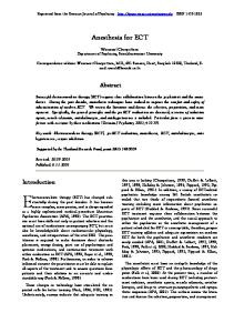
we are assuming that an entrepreneur learns about ideas for sale through all the agents working in his …rm, including himself. This may be the result of workers having ideas themselves and selling them to their employer, as that may be easier than contracting with an unknown entrepreneur. Alternatively, one may think of employees …nding out about ideas for sale in the market and informing their employer. Figure 1 summarizes what we have learned about …rm behavior and …rm entry. It shows expected revenue
in the real line. For projects above
…rms implement ideas with ’s between
L
and
H.
H,
…rms’ workers spin o¤. All other
An incumbent risk-neutral entrepreneur would
implement projects as long as they pay expected return w, so the di¤erence between
L
and w is
the result of an entrepreneur’s ability to drop the project next period (this ordering can change In the particular case in which ( ; N ) = ~ ( )N and utility is linear, even without the market for ideas, L is independent of size. The market for ideas is necessary to obtain scale independence in the selection of ideas if the utility function is not linear and/or ( ; ) is not linear in N: In Appendix A, where we consider the case of exponential utility, this is evident. 11
14
Figure 1: Selection of Ideas
once we consider risk-averse agents). The threshold that determines L is given by Z Z (P w) dF L (P ) = 0: (P w) dF L (P ) + 1 w The di¤erence between
L
and
H
(5)
is the result of the option value of exiting and setting up a new
…rm in the future, f0 . The threshold H is implicitly determined by Z Z (P w) dF H (P ) + (P w f0 ) dF 1 PH The value of having ideas for the worker is given by Z Z Z f0 = max (P w) F (P ) + max [P w 1
H
(P ) = Z:
f0 ; 0] dF (P ); 0 dH( ) + (1
(6)
)Z: (7)
This value includes the option to spin o¤ and start a new …rm and therefore give away the chance to spin o¤ with a better idea, as well as the expected value of the ideas sold in the market Z. The di¤erence between the two thresholds comes from the option value, included in f0 ; of closing a new …rm and starting another one later on with a better idea and the fact that workers give up the price of an idea Z when they set up the …rm. Note that if f0 = 0, the two threshold equations and the equation for Z imply that Z = 0 and
L
=
H:
So, all projects would be implemented via spino¤s.
However, as shown in the previous proposition, f0 is positive, since workers can extract the value of very good projects by spinning o¤. New …rms will require a higher return from their …rst project than existing …rms demand from new projects, given the larger option value f0 that new …rms have of returning to an old …rm and spinning o¤ in the future, namely, PH > w = PL :12 Both of these equations imply that the number of entrants as a fraction of the population is constant and so is the number of new projects implemented in existing …rms each period as a fraction of total 12
See Appendix B, where the di¤erence between equations (5) and (6) is not f0 but an exogenous entry cost f:
15
population.13 These results depend on the assumption that project returns are speci…c to the entrepreneur who implement the idea. If project returns were not entrepreneur speci…c, then a worker who found that his project has a payo¤ between w and PH could sell that project to an established …rm. Then, workers will not be any more selective in implementing ideas than established …rms and
H
=
L;
but it would still be the case that PH > w = PL : Finding an equilibrium amounts to solving equations (4), (5), (6) and (7) for the values of Z; f0 ;
L
and
H;
and the market clearing condition (3) for : The next proposition establishes that
an equilibrium exists and is unique.
Proposition 6 A long-run equilibrium for this economy exists and is unique
As we noted above, one potential issue is the existence of an equilibrium with contingent contracts, namely, a contract in which an entrepreneur o¤ers the worker the contingent return on an idea minus w. We can now be more speci…c about how big these costs of writing contingent contracts need to be for such contracts not to be used. Workers with good ideas that would otherwise spin o¤ would be willing to stay if the cost of writing a payo¤-contingent contract that mimics what the worker gets by spinning o¤ costs less than f0 : Note that this includes everything the worker gives up by spinning o¤. Namely, the market price of his future ideas as well as the option to spin o¤ in the future with a better idea. In Appendix A, we show that all results, except according to u (ct ) =
ae
bct .
L
< w; hold when individuals order preferences
In this case all agents in the economy are risk averse. However,
because their risk aversion does not depend on the level of their wealth, in the presence of markets for ideas, we still obtain the result that
L
is constant, and therefore that the selection of ideas
and projects is scale independent as before. All other details, including an explicit formula for the equilibrium price of an idea, are relegated to Appendix A. 13
Note that PH > w implies that a project dropped by a spino¤ could be sold to existing …rms. Since we have assumed that projects are speci…c to the entrepreneur, we have abstracted from these transactions. We could relax this by assuming that projects can be sold at some cost. This would lead to a situation where some projects are sold at market value to existing …rms. If we assume that projects can be sold at some cost, the agent who is deciding whether to carry on as an entrepreneur will decide to do so if the cost of selling the existing project is greater than the value of being a worker and having the option to spin o¤ in the future. Then, this model would have both a market for ideas and a market for start-ups. Importantly, it will not eliminate the market of ideas which is the focus of this paper.
16
4
Comparative Statics, Empirical Implications, and Evidence
Our theory determines the selection thresholds
L
and
H,
the market price of ideas Z; and the
option value of spinning o¤ f0 . These equilibrium values depend on the di¤erent parameters of the model, namely, the discount factor , the probability of having ideas , the outside wage w, as well as the distributions of realizations given an idea; F , and the distribution of the quality of ideas, H. With linear utility, no other parameters enter the model. Given the values of (
L;
H ; Z; f0 )
the model also yields implications on the size distribution of …rms, …rm growth rate, the number of spino¤s, and other distributional outcomes. Important for our purposes is that none of the latter implications have to be solved for in order to obtain (
L;
H ; Z; f0 ).
We can solve the model
sequentially because the value of ideas, both within existing …rms and in new …rms, do not depend in equilibrium on the distribution of …rm sizes in the economy. We turn to the implications on the size distribution of …rms and other outcomes in the next section. The values of (
L;
H ; Z; f0 )
(5) it is immediate that L
L
are determined by Equations (4), (5), (6), and (7). From Equation
is decreasing in , independent of , and increasing in w. Furthermore,
decreases if we switch from F to F 0 where F 0 …rst order stochastically dominates F .
L
is independent of the distribution H. Hence, …rms are more selective as wages increase, but less selective if agents are more patient or if the distribution of realization of a given idea improves. The e¤ect of parameters on the other equilibrium values is much more complex, as the system is only block-recursive for simulations we let F (P ) = length
L . We therefore P ( =2)
proceed with numerical simulations. In all numerical
. Namely, we let F be a Uniform distribution with range of
centered at . For H we use a Generalized Pareto distribution with minimum value given
by 1 and shape coe¢ cient given by . That is H( )=1 So a higher
(1 + (
1))
1=
:
implies that the distribution has a left tail with more mass.
Given these two distributional assumptions, we need to pick 5 parameters. We let standard value for yearly data. We will show comparative statics for the values of !; let
= 0:95: a and . We
= 8; which, given the ranges of the other three parameters, gives us realistic ratios of new
employees in new …rms relative to new employees in continuing …rms. This statistic is the only moment that matters to determine the size distribution of …rms and other distributional outcomes, as we argue in the next section. We denote this statistic
H= L
and calculate it to be between 0:07
and 0:12 in the US economy from 1989 to 2003 (we discuss the details of this calculation in the 17
2 1.5
13
12
12.5
11.5
12
11
Z
µ
µ
L
H
1 0.5 11.5
0 -0.5 4
10.5
11 6 2
0.65
10 6 5
-3
6 4 λ
2
0.55
2
0.55
0.65 4
x 10
0.6
3 λ
σ
5 -3
4
x 10
0.6
0.65
0.6
3 λ
σ
2
0.55
σ
-4
x 10
11
10.5
10 6 5 -3
x 10
0.1
2
0.095
1.5 1
0.085 0.08 6 5
-3
3 λ
x 10
0.6 2
0.55
0.09
0.5 6
0.65 4
L
0.105
H
f
0
11.5
3 2.5
λ / λ
N umber of Spinoffs per Worker
12
0.65 x 10
0.6
3 λ
σ
5 -3
4 2
0.55
0.6
3 λ
σ
Figure 2: Comparative Statics for
0.65 4 2
0.55
σ
and
next section). Figure 2 shows the value of (
L;
H ; Z; f0 )
as a function of
and . We choose a range of
that makes a worker have between 0:2% and 0:6% probability of having an idea each period. So a …rm with 1000 employees will have 2 to 6 ideas per year. The range of values of
that we choose
makes agents spin o¤ with about 3% of those ideas. They also show the number of spino¤s per period per worker, and the
H= L
ratio discussed above. As one can see in the …gure, the ratio of
new employees in new …rms to new employees in continuing …rms is in the relevant range for these parameter values. Several results are noteworthy. As
increases, we shift more mass to the tail of the distribution
H: This implies that good ideas are more likely. As noted above this does not a¤ect how selective continuing …rms are in choosing which projects to implement,
18
L,
but it does imply that workers
wait longer for better ideas to spin o¤. As
increases, we also …nd that the price of ideas increases,
since the average idea sold in the market is now of better quality. This is because both
H
went
up and there is more mass in the left tail of the distribution. The option value of setting up a new …rm, f0 , also goes up. An increase in as
has similar e¤ects, although (in this exercise) smaller in magnitude. First,
increases, the values of
H,
Z and f0 all go up. This means that a higher probability of
generating ideas leads to more selection of ideas by potential entrepreneurs. Since …rms’selection of implemented projects of projects (
H
L
projects (higher
H)
L
does not vary with , this means that …rms implement a wider range
grows). Note that even though workers are more selective in their choice of there are more spino¤s per worker. The e¤ect of
is hard to assess in Figure
2, so we show this dimension separately in Figure 3.
11.7 11.6 11.5 µ
H
µ , Z and F
0
11.4
H
Z F
11.3
0
11.2 11.1 11 10.9 10.8 10.7 2
2.5
3
3.5
4 λ
4.5
5
5.5
6 -3
x 10
Figure 3: The e¤ect of
Figure 4 shows the same six graphs presented in Figure 2, but we change the axes to re‡ect 19
changes in the wage w rather than the shape parameter of the Generalized Pareto distribution, : The …gure shows similar comparative statics for
as described above. The e¤ect of higher
outside wages follows a di¤erent pattern. Higher w implies more selection by …rms as is easy to show analytically (higher
L ).
Furthermore, a higher w reduces
H;
Z and f0 but it increases the
number of spino¤s and the ratio of lambdas. So if workers are more expensive, …rms will implement a smaller range of projects. Since on average the ideas sold to …rms are worse, the price of ideas falls as does the option value of an idea. As the threshold
H
decreases with the increase in w,
more ideas lead to spino¤s and, given the number of ideas per person , there are more spino¤s per person. This also implies that the number of new employees in new …rms grows relative to the number of new employees in continuing …rms and so
H= L
increases as well.
14 13 13
1.3
12
1.2
12
11
1.1 11
10
0.9
Z
µ
H
µ
L
1
10
9
9
8
8
7
0.8 0.7 6 5 -3
x 10
6.2
4 λ
6 6
7 6
6.1 2
5.9 5.8
4
-3
6
x 10
w
6.2 5
6.2
6
3
2
λ
6
4
-3
3
x 10
5.8
2
λ
w
5.8
w
-4
x 10
13
9 8 7
0.2
2
0.15
1
0.1
0 6
0.05 6 5
6 6 -3
3
H
f
0
10
0.25
λ / λ
11
4
L
Number of Spinoffs per Worker
12
-3
4
x 10
λ
2
5.8
5.9
6 w
6.1
6.2
x 10
5 6.2
4
6.1 2
6.1 6
3
5.9 5.8
6.2
4
6
3 λ
-3
x 10
λ
w
Figure 4: Comparative Statics for
2
5.9 5.8
w
and w
We now discuss the evidence in support of the implications of our theory. The empirical literature on spino¤s has identi…ed several regularities. An important regularity seems to be that 20
"employees start their own …rms after becoming frustrated with their employers. Their frustration is often related to having an idea about an innovation or a new (sub)market rejected by their employer" (Klepper and Sleeper, 2005). In our paper, disagreements mean that parties cannot …nd a price at which they can transact. This is the core implication of our way of modelling incomplete information. Perhaps, the most important implication of our framework is that only the best ideas lead to spino¤s. Therefore, we should observe in the cross-section that the …rst idea of a …rm is in general better than future ideas. This is consistent with some of the available evidence, which suggests that the …rst product of a …rm is, on average, the most successful of its products. Prusa and Schmitz (1994) argue that this is the case in the PC software industry. The …rst product of a …rm sells, on average, 1:86 times the mean product in its cohort, while the second product sells only 0:91 times the mean product in its cohort. That is, …rst products are, on average, about twice as successful as second products. The …rst product is also about twice as successful as the third, fourth, and …fth products. This evidence suggests that spino¤s discriminate more than incumbent …rms in choosing which projects to implement. This is exactly in line with the selection mechanism our theory underscores. Another related …nding is the evidence in Luttmer (2008) that new …rms need to draw from a better distribution in order to explain the age distribution of …rms. The model also predicts the fraction of unsuccessful spino¤s that exit the economy. Large …rms can have unsuccessful projects, too, but they do not exit; they just drop the project. They do not exit, since they have at least one ongoing project that provides a permanent source of pro…ts. Some authors (for instance, Hall and Woodward, 2007) have argued that a common phenomenon is for workers to spin o¤ only to be acquired by a larger …rm some years later. Our theory provides a rationale, namely, adverse selection, for why we have spino¤s, but we do not address the issue of spino¤s being acquired by existing …rms later on. The theory also has predictions for the entry process of …rms. Large …rms generate more spino¤s than small …rms, although as a fraction of the workforce, the number of spino¤s is constant. This is consistent with the evidence discussed in Klepper and Sleeper (2005) that …rms that produce a wider range of products generated more spino¤s over time. Franco and Filson (2006) show, for the hard-drive industry, that more know-how (which is likely correlated with size) also leads to more spino¤s. Our numerical simulations in the previous subsection generated several other empirical implications. In particular, parameters that could be related to better economic circumstances, like
or
; imply a higher threshold to spin o¤, more spino¤s, a higher price of ideas, a higher option value of spinning o¤ and proportionately more new workers entering through spino¤s. These predictions 21
of the model are particularly relevant in light of the empirical facts in Jovanovic and Rousseau (2009). They document that the aggregate Tobin’s Q is positively related to the skill premium, negatively related to the relative investment of incumbents, and positively related to the number of spino¤s. High aggregate Tobin’s Q can be compared to times in which many agents have ideas. Or times where
is high: times where
is high: times where ideas are particularly good. Given
this, our model predicts that in fact we should see more spino¤s, a higher value of the option to spin o¤, a higher market price of ideas –which could be compared to the skill premium where the skilled are the agents with ideas – and less investment by incumbents relative to new …rms, as is evident by the increase in
H = L.
Similarly, the previous section illustrates the predictions of the model for how these variables change with respect to outside wages. In particular, the model implies that the price of ideas decreases with wages, the number of spino¤s increases, and the entry of new workers through new …rms increases as well. We do not know of empirical work that has contrasted these types of implications with data but these are implications of our model that can be potentially tested. As we show in the remainder of the paper, the implications of all of these parameters for the ratio of H= L
are particularly relevant as they are directly related to the shape of the size distribution of
…rms. We now turn to these implications of the model and examine how they compare with the data.
5
Invariant Distribution of Firm Sizes: Theory and Evidence
In order to derive the implications of our model for …rm growth and the size distribution of …rms, we need to take a stand on the number of projects that …rms …nd out about. The reason is that in our model, given the price in the competitive market for ideas, entrepreneurs are indi¤erent about how many ideas to buy. This implies, as argued above, that we need to specify the function ~ ( ) : Assume that entrepreneurs encounter ideas in proportion to the number of agents in the …rm. This amounts to assuming that they …nd out about ideas generated by agents in their own …rm or, alternatively, they and their workers get information about ideas at a constant rate per person. Suppose that a …rm with N projects has a probability of …nding out about an idea given by ~ ( ; N ) = N: We assume that the maximum size of a …rm is given by N such that N < 1.14 14
Alternatively we could work with continuous time and assume that the process by which …rms generate ideas is Poisson with parameter N . This would imply an identical random process for generating ideas in continuous time. Note that we are assuming that the process of generating ideas and the process of assigning knowledge and ownership
22
Everyone in the …rm has a probability of
> 0 of generating an idea. Note that since the value
depends on our de…nition of a period, we can always make
small enough by appropriately
de…ning the length of a period in the model. Correspondingly, we can make N arbitrarily large. In case a …rm hits the size constraint N , its workers will sell ideas to other …rms. For the moment we abstract from this problem, but we return to it below. One way to justify our choice of
( ; N) =
N is to assume that an entrepreneur can only
evaluate one idea per period. Then, if he confronts ideas from each of his workers with probability ; the probability of evaluating an idea in any period is multinomially distributed and given by 1
(1
)N : Taking a linear approximation at
entrepreneur having access to an idea is given by
= 0; yields that the probability of an
N . Of course, this approximation works well
when we are faraway from the upper bound N = 1= : Otherwise, we would need to work directly with 1
(1
)N which would complicate the analysis but would avoid having to impose an
arbitrary upper bound. As we have shown, entrepreneurs are indi¤erent about how many ideas to buy in the market. Thus, in combination, this speci…cation of ~ ( ) implies that the growth of …rms will be independent of size (Gibrat’s Law). It is important to note, however, that Gibrat’s Law is not su¢ cient to determine the form of the invariant distribution of …rm sizes. The latter depends on the process of entry and exit. For example, as Gabaix (1999) shows, Gibrat’s Law with no entry and exit and a re‡ecting barrier arbitrarily close to size 0 leads to a Pareto distribution with coe¢ cient 1: In contrast, in Eeckhout (2004) Gibrat’s Law with no entry (of cities) and no re‡ecting barrier leads to a Log Normal distribution in the limit. In our case, the total mass of …rms is also normalized to 1 –which is equivalent to having exit at a proportional rate –but there will be entry at size 1. This, as we show below, leads to a Yule distribution for …rm sizes, which …ts the …rm size data well (as shown before by Simon and Bonini (1958)). In this sense, it is the entry process that distinguishes our theory from other theories of …rm dynamics that are also consistent with Gibrat’s Law. Given our speci…cation for ~ ( ) we need to determine demand for ideas equalize in equilibrium at price Z: Let
such that the supply of ideas and the N
denote the share of …rms of size N in
equilibrium (we will discuss this distribution in much more detail below). Then, market clearing in the market for ideas requires 1 X
(N
1)
N
=
N =1
1 X
N
N;
(8)
N =1
are independent. If instead each worker had an unconditional probability of generating an idea independently of other workers, there would be a positive probability of generating several ideas per period, which we rule out.
23
where the l.h.s. is the supply of ideas (N
1 workers in a …rm of size N have a probability
generating an idea) and the r.h.s. is the demand for ideas (a …rm of size N learns of ideas). Denote by
( ; N) =
of N
the average …rm size, then =1
1
:
(9)
That is, the number of ideas per worker encountered by an average entrepreneur is equal to Each worker has a probability
:
of having an idea. Since entrepreneurs do not have ideas, on
average each entrepreneur is confronted with a probability of encountering an idea that is lower than ; namely
: Thus, intuitively,
is just unity minus the share of entrepreneurs in the total
number of people working in the industry (1= ).15 Note that our assumption that the maximum size of …rms is given by N implies an additional adjustment for : Since …rms get zero expected bene…ts out of implementing ideas, entrepreneurs are indi¤erent about expanding or not. Hence, they do not care about this upper bound for the size of their …rm. The only role that this bound plays is to determine how other …rms grow if there is a positive mass of constrained …rms. Thus, the only adjustment we need to make is to add the upper bound N to equation (8). Notice, however, that equation (9) still holds. In order to derive the size distribution of …rms, …rst note that the size of the industry will increase constantly in our setup since innovation does not stop (every worker in the industry has probability
of having an idea independently of where they work). The probability of …rms adding
a project is positive for all …rms, while the probability of dropping a project that is already being used is zero. Hence, …rms will only grow over time. This is combined with a positive mass of new entrants with one worker every period. So we can show only that there is an invariant distribution of employment shares and …rm sizes measured as a share of total employment. That is, we normalize by the size of total employment. This normalization is equivalent to having an exogenous death rate independent of size.16 First, consider the transition equation for a …rm with N workers. Each worker has a probability of having an idea. If they do, the …rm implements it if
2[
H;
L (N )]
and if it implements it,
15 Since entrepreneurs do not get ideas, a new …rm with only one worker will need to buy an idea from a nonemployee to grow. More generally, small …rms will need to buy ideas from non-employees in order to grow at the same rate as large …rms. The number of ideas originating in a …rm that are sold to outside entrepreneurs, as a proportion of the number of workers in the …rm, is given by [(1 1=N ) ] = [1= 1=N ]: 16 In our model, …rms die for two di¤erent reasons. First, new …rms may …nd out that their productivity is low and exit. Second, as described in the text, we normalize the total mass of …rms to one. This is equivalent to assuming that exit rates of continuing …rms are independent of size. Thus, in a stylized way, we do incorporate the feature that exit rates are decreasing in size.
24
the …rm uses the idea with probability 1 W
F (PL (N )) where PL (N ) is such that
N S + PL (N ) ;N + 1 N +1
= W (S; N );
which by the arguments above does not depend on S. In what follows we will ignore the upper bound on …rm sizes N : We will return to it once we de…ne the invariant distribution of …rm sizes for the case without this bound. Hence if p (N; N + 1) denotes the probability of a …rm transitioning from N to N + 1 workers Z H (1 F (PL )) dH ( ) : p (N; N + 1) = N L
Hence,
p N; N
0
=
8 > 0 > > > > > < > > 1 > > > > : 0
R N h
for N 0 > N + 1 H L
N
Let S = f1; 2; :::g ; then, for any A
(1 R
F (PL )) dH ( )
for N 0 = N + 1
(1
for N 0 = N
H L
i F (PL )) dH ( )
:
for N 0 < N
S, X
p (N; A) =
p N; N 0
N 0 2A
is positive if N 2 A or N + 1 2 A. Let Lt be the total labor force and Et the total number of …rms or enterprises in period t; and let f
Ng
be the invariant distribution of …rm sizes. The probability that a …rm with N employees
generates a spino¤ is given by s (N ) =
N
Z
(1
F (PH )) dH ( )
H
where PH satis…es W (PH ; 1) = W0 : Hence, the expected number of spino¤s in period t + 1 given the distribution of …rm sizes in period t is given by Et
NX =1
s (N )
N =1
=
Z
(1
N
= Et
Z
(1
F (PH )) dH ( )
N =1
H
F (PH )) dH ( ) Lt
H
25
NX =1
H Lt ;
N
N
where
H
denotes the number of new employees in new …rms as a fraction of total employment.
Hence the expected number of spino¤s is a constant fraction of the population, Lt . Similarly we can calculate the expected number of new workers in existing …rms, which is given by Et
Lt X
p (N; N + 1)
N =1 Lt X
L Et
N
= Et
Lt X
Z
N
N =1
N
N
=
H
(1
F (PL )) dH ( )
N
L
L Lt ;
N =1
where
L
denotes the number of new employees in old …rms as a fraction of total employment.
Then, for Et large Lt+1 = Lt + Et
Lt X
[p (N; N + 1) + s (N )]
N
= (1 +
H ) Lt
+
L Lt :
N =1
Given our de…nition of
L
and
H,
population evolves according to
Lt+1 = (1 + Thus, Et+1 = Et + Et
1 X
H
+
s (N )
L ) Lt
N
= Et +
H Lt :
N =1
Hence the number of …rms is expanding at a constant rate. In terms of the number of …rms, the economy is growing at a constant rate. Note that we are assuming that Et is large enough so that Lt and Et evolve deterministically. For small Lt and Et , however, both are random variables that evolve according to a stochastic process. We now compute the invariant distribution of the share of workers in …rms of di¤erent sizes. Let
N
denote the probability that a worker is employed by a …rm with N workers. The probability
that a worker has an idea that is used within the …rm is given by
L;
independently of the …rm’s
size. Then, the invariant distribution satis…es [
1 (1
L)
+
H] L
=
0 1L
=
1 (1
+
L
+
or 1 (1
L)
+
H
= 26
1 (1
+
L
+
H)
H) L
which implies 1
H
=
:
+2
H
(10)
L
Intuitively, the number of workers in …rms of size 1 today, …rms of size 1 that become workers in …rms of size 2, …rms of size 1, 1 tomorrow, is
L
+
H L, 0 1L ,
1 L;
1 L L,
minus the number of workers in
plus the number of new workers in
is equal (in the invariant distribution) to the number of workers in …rms of size
which is equal to
1 (1
+
+
L
H ) L;
given that the growth rate of employment
H:
Similarly, for …rms of size N;
=
N
(1
LN )
N
(1 +
L
+
+
N 1 L (N
1) +
=
N 1 L
N
(1
LN )
+
N 1 LN
H)
and so N
LN
=
N 1
H
+
L (N
(11)
+ 1)
which implies that N
N
L (N
N 1
=
N
1
H
1) : (N + 1) L
+
Note that by de…nition (1 +
L
+
H)
1 X
N
=
1 X
N
(1
LN )
+
N 1 L (N
1) +
N 1 L
N =2
N =1
+
1 (1
L)
+
H
which implies that (
L
+
H)
1 X
N =1
Hence,
N
=
"
1 X
N 1 L
+
N =2
1 X
N
H
#
=
L
1 X
N
+
H
N =1
= 1;
N =1
and so the resulting ’s form a probability distribution. This distribution is the invariant distribution of employment shares across …rms of di¤erent sizes.
Proposition 7 There exists a unique invariant distribution sizes, where
N
of employment shares across …rm
denotes the share of workers employed by …rms of size N .
27
To obtain the distribution of …rm sizes we need to transform the distribution of worker shares into a distribution of …rm sizes. For this, note that if the share of the population employed by …rms of size N is given by
N,
then the share of …rms of size N; =
N
Clearly, since
P1
N =1
N
= 1, 0 <
P1
N
N
P1
N
is given by
:
(12)
N =1 N
< 1 and so
N
N =1 N
N;
is well de…ned, exists, and is unique.
N
Since we are normalizing the total mass of the size distribution to one we are, in e¤ect, introducing exit at a constant rate for all sizes.
Corollary 8 There exists a unique invariant distribution
of …rm sizes.
Simon and Bonini (1958) propose an exogenous growth and entry process of …rms that leads to the same type of distribution, namely, a Yule distribution. This distribution approximates a Pareto in the upper tail. Note from the previous equations that the distributions only on the value of the ratio
H = L.
a microfoundation for the value of
and
depend
So, one of the contributions of our theory is to provide
H= L
that in Simon and Bonini (1958) is just an exogenous
parameter. Note also that in the theory N
N . Hence, in order to get distributions of employment shares
and …rm sizes that are consistent with the theory we need to re-normalize both distributions. Hence, the distribution of employment shares is given by ~
N
=P N
N
N =1
and the distribution of …rm sizes by
~N = N
N
~ N PN
~ N N =1 N
:
Now consider the expected growth rate of employment, gN ; of a …rm of employment size N . The …rm grows by one employee with probability N gN =
(N + 1) N
L
+ N (1 N
L,
thus
N
L)
N
=
L:
Hence, the expected growth rate of …rms is just given by the probability per worker of its employees generating an idea that is used. This probability is constant, so the expected growth rate in terms of 28
employees of existing …rms is constant, which is a statement of Gibrat’s Law. Therefore, the model is consistent with the evidence in Sutton (1997), who argues that the unconditional (on survival) growth rate is consistent with Gibrat’s Law. Of course, this is the result of our assumption that ( ; N ) / N ; however, we were free to assume this, given that the market for ideas implies that
…rms with di¤erent characteristics select ideas identically. For our purposes, whether Gibrat’s Law
holds exactly or not is not crucial. What we will show is that using Gibrat’s Law we can approximate the size distribution well. However, we can incorporate any pattern of scale dependence in growth rates and use the model to generate implications for the size distribution. The model has another relevant implication. Since employment grows by one unit at a time, the variance of the growth rate of employment is decreasing in N: In particular, the variance of the growth rate of employment is given by 1 + 2 (1 N
L)
L
+ (1
2 L)
which is decreasing in N: Gabaix (2005) documents that the volatility of …rm growth rates decreases with size with an elasticity between 0.15 and 0.20. Our model implies a volatility that also declines with size but not with a constant elasticity. Proposition 9 The expected growth rate in employment size of existing …rms is independent of their size. Furthermore, the variance of …rm employment growth is decreasing in …rm size.
Similarly, the expected growth rate in average revenue of a …rm with average revenue S and N employees is given by N gS;N
= = =
This implies, as
L
N N +1
R
R
1 N +1
H L
H L
"
R1
N S+P N +1
PL
R1 PL
S
Z
dF (P ) dH ( ) + S (1
N
L)
S
NS P dF (P ) dH ( ) + H
L
Z
NS N +1
N
L
NS 1
P dF (P ) dH ( )
PL
and PL , and therefore
L;
L
#
+ S (1
N
L)
S
:
are independent of N that
ES (gS;N ) = 0: So average growth rates across …rms of di¤erent average revenues are zero. However, large …rms that have had good realizations and therefore have a high S will tend to grow slower, and vice 29
versa. In this sense there will be reversion to the mean, conditional on the number of employees. This is consistent with Luttmer (2008), who argues that a higher rate of growth for young (and small) …rms is key in explaining the age distribution of …rms. Our paper complements Luttmer (2008) by providing a micro-founded model of why this is the case. Also note that the variance of gS (S; N ) is decreasing in N , since the larger the …rm, the smaller the contribution of new projects (see also Proposition 9 and Gabaix (2005)). Since …rms implement projects that yield only non-negative pro…ts, this implies that the growth rate of total revenue or total pro…ts will decline with size. Note that since N
it is immediate that as N ! 1 or
=
LN N 1
H
+
L (N
! 0; when N ! N ,
+ 1) N
N 1;
so the share of workers at
large …rms is approximately constant. This implies that the density of …rm sizes will be proportional to 1=N as N becomes large. That is, the tail of the distribution will be arbitrarily close to the tails of a Pareto distribution with coe¢ cient one. Similarly if and so for N large
N
N 1
H
is small,
N
N 1 (N= (N
+ 1)) ;
and the distribution of …rm sizes is approximately Pareto with
coe¢ cient one. This is interesting given that several authors have concluded that the upper tail of the distribution of …rm sizes is close to a Pareto distribution with coe¢ cient one (see, for example, Axtell (2001)). We summarize these results in the following proposition.
Proposition 10 As
! 0, or N ! 1; the density of …rm sizes is arbitrarily close to the density of
a Pareto distribution with coe¢ cient one, for large enough …rm sizes. Furthermore, the distribution
of …rm sizes is closer to a Pareto distribution with coe¢ cient one, the smaller the mass of workers in new …rms,
H:
The invariant distribution of …rm sizes, as well as any other outcome of the model, is a function of the exogenous parameters and distributions in the model, namely,
, w; and the distributions
F and H. However, as we show above, the e¤ect of all those variables can be summarized through the value of
L
and
H = L:
Therefore we can assign a particular value to this ratio and compute
the resulting distribution of employment shares and …rm sizes. Figure 5 illustrates the invariant distribution in this model and compares it with the distribution of …rm sizes in 2000 in the US. The data for the distribution of enterprises come from the Statistics of US Businesses (SUSB) program. These data cover the whole private US economy (except agriculture) and were constructed by the
30
US Census Bureau for the study in Rossi-Hansberg and Wright (2007).17 In this paper we make use of the evidence on enterprises rather than the evidence on establishments which is the focus of Rossi-Hansberg and Wright (2007). Apart from the size distribution of …rms for the aggregate economy, the data set includes the size distribution of enterprises at the two-digit NAICS level for 2000, which we also use below. The industry data are provided for enterprises of up to 10000 employees. In order to compute the distribution given in equation (12), we need to truncate the distribution of …rm sizes at a certain size. We choose N = 500000; since the largest …rms reported in the aggregate data have this number of employees. We choose
H= L
= 1=9 and so 90% of the new
employees are hired by existing …rms and 10% by new …rms. As is evident from equations (10) and (11), the distribution depends only on the ratio
H= L
and not on
H
and
L
separately.
Figure 5 shows how our model can do a good job in matching the distribution of …rm sizes. Relative to a Pareto distribution with coe¢ cient one (a straight line with slope minus one), it exhibits a relatively thinner tail of small …rms. Furthermore, since in the model and in the data we are truncating the distribution, both distributions exhibit thinner tails than the Pareto distribution for very large sizes. This is only the result of truncation in the model. If we let N ! 1, then the theory implies that the upper tail will be arbitrarily close to the Pareto distribution for large enough sizes. Similarly, in the data the census does not reveal the sizes of the largest …rms because of con…dentiality concerns. Furthermore, while in the model we do not have integer constraints and so there are some …rms at all sizes, in the data there cannot be any fractional …rms, which truncates the distribution as well. Hence, the reason to have a small mass of large …rms on the upper tail is similar in the model and the data. One noticeable di¤erence between the distribution generated by the model and the distribution generated in the data is that the theoretical distribution lies below the empirical one in Figure 5. The reason for this is that in our setup, ideas are generated by one employee and not by teams of employees. Consequently, individual agents spin o¤, not teams of agents. This is clearly not true in the data. Firms enter small, but not necessarily with one employee. Were we to assume that teams of between 2 and 3 employees have ideas and spin o¤, we could shift the theoretical curve in Figure 5 so that it lies on top of the empirical one. Thus, the emphasis is on the shape, not the level of the curves. This exercise is illustrated in Figure 6. 17
Rossi-Hansberg and Wright (2007) discusses the important di¤erences observed in the size distribution of establishments and enterprises (…rms). Their paper is solely concerned with establishments, while the current paper is about …rms.
31
0
-2
ln ( Prob. > Employment)
-4
-6
-8
-10
Model: Employment Shares Model: Firm Size Distribution
-12
Data: Firm Size Distribution
-14
-16
0
2
4
6 ln (Employment)
8
10
12
Figure 5: Model vs. Data
Figure 6 uses a value of
H= L
= 0:0736. This value is the empirical counterpart of
H= L
in the US economy from 1989 to 2003. Namely, we calculated the net number of workers added by new …rms and divided it by the net number of workers added by continuing …rms. The data come from the US Small Business Administration (SBA). If we instead calculate the ratio for each year and average over time,
H= L
increases to 0:1235: Clearly, the model does a very good job of
matching the aggregate distribution, arguably better than a Pareto distribution at the upper and lower tails. Figure 7 shows how we can modify the shape of the invariant distribution by changing the ratio H = L.
We illustrate this using N = 10000: The relationship between
H= L
and the primitives
of the model is discussed in Section 4. Here, we simply display the invariant distribution for H= L
= 1=2; 1=5, 1=10, and 1=20: It is clear from the …gure that as we increase the number of 32
0 Data: Firm Size Distribution Model: Firm Size Distribution (Teams of Size 2.5) -2
ln ( Prob. > Employment)
-4
-6
-8
-10
-12
-14
-16
0
2
4
6 ln (Employment)
8
10
12
Figure 6: Model vs. Data with Variable Team Size
entrants (by increasing
H = L );
we shift mass to the lower tail, and therefore, the slope of the
curve in Figure 7 becomes steeper. However, as we know from the previous proposition, if one increases N to large enough values, the shape of the distribution approaches a Pareto distribution, as N increases, in all these cases. Figure 7 illustrates the invariant distribution for a large range of parameters. The empirical value of
H= L
is as calculated above, equal to 0:0736.
The next step is to assess whether the relationship between
H= L
and the size distribution of
…rms can explain some of the variation in the size distribution of enterprises across sectors. Di¤erent sectors have di¤erent values of
H = L.
This, according to our model, should explain some of the
variation in the distribution of enterprise sizes in the data. There are two main issues in performing this exercise. The …rst is that the data to calculate
33
0 Pareto with coeffic ient one
λ / λ = 1/2 H
L
λ / λ = 1/5 H
L
λ / λ = 1/10 H
L
λ / λ = 1/20 H
L
λ / λ = 1/50 H
L
ln (Prob. > Employment)
-5
-10
-15
0
1
2
3
4
5 ln (Employment)
Figure 7: The E¤ect of
H= L
6
7
8
9
10
H= L
for enterprises at the two-digit NAICS level are not publicly available. There are data
provided by the US SBA to do this for establishments, but aggregating to enterprises is not trivial. Furthermore, the data for establishments will, in general, show relatively more new net employment in new establishments than in continuing establishments compared to the enterprise data. This occurs since continuing enterprises may add new employees by adding a new establishment. Hence, H= L
calculated with establishment data will be larger than with enterprise data. Given the
available data, we can compute this measure for the aggregate economy for both enterprises and establishments. In fact, our calculations show that the ratio for establishments is about 10 times larger than for enterprises. This provides a measure of the bias when we use establishment data instead of enterprise data. We can then compute
H= L
using establishment data for each two-digit
NAICS industry and multiply them by the ratio of the measure of
H= L
for enterprises divided by
the one for establishments for the aggregate economy. This provides us with an estimated measure
34
of
H= L
for enterprises in all two-digit NAICS industries.
The second issue is that we need a benchmark to compare our results. In particular, we need to assess if the model can explain some of the variation in the observed size distribution of enterprises across industries. We use the aggregate observed distribution of enterprises as our benchmark. So we compare the average absolute distance between the industry size distribution of establishments and the aggregate one in the data. We then compute the size distribution predicted by the model if we use the industry
H= L
calculated as described above. We need to do one more adjustment.
From our discussion of Figures 5 and 6, it is clear that in order to match the level of the size distribution of enterprises we need to adjust the size of the teams that can have an idea and implement it. We saw in Figure 6 that a team of 2.5 workers does a good job for the aggregate economy. However, the required minimum team size probably varies substantially across industries. To address this we choose the team size for each industry so as to minimize the average absolute deviation between the model’s implied distribution and the industry distribution of enterprises. Figures 8 and 9 show the results of this exercise for 19 two-digit NAICS industries and the aggregate economy. For all industries we set the upper bound on …rm size, N , equal to 20000, although our calculations do not change signi…cantly if we choose numbers between 10000 and 30000. The data is censored at 10000, so 20000 seems reasonable. The …gure for the total economy is almost identical to Figure 6, except that the estimated team size is actually 2.72 not 2.5 as in that …gure. The …gures include the estimated team size for each industry, which varies from 1 in the ‘Accommodation and Food Services Industry’to 403 for ‘Management of Companies and Enterprises’(a clear outlier given the shape of the distribution of enterprises in this industry. The second largest team size is 16.4 for ‘Utilities’). We also report the average absolute di¤erence between the modeled distribution and the data and the aggregate distribution and the industry data. The model beats the aggregate benchmark in 14 out of 19 industries. It does a particularly good job in matching the distribution in ‘Manufacturing’, ‘Educational Services’and ‘Health Care and Social Assistance’. We conclude that although certainly not the only source of variation,
H= L
explains part of the industry variation in the size distribution
of …rms. As discussed above, in computing the distributions predicted by the model for the observed H= L
in each industry, we also estimated the size of the implied team sizes across industries,
namely, the size of the team that makes the model …t the industry data as closely as possible. It is then a natural question whether the team sizes implied by the model via the exercises performed
35
Modeled Industry Firm Size Distribution
Indus try Firm Size Distribution
T otal 0
ln (Prob. > Emp.)
ln (Prob. > Emp.)
0 -2 -4 T eam Size:2.72 -6
Avg Model Diff. =0.12483 Avg Economy Diff. =0
-8 -10
0
2
4 6 ln (Employment) Mining
-4 T eam Size:11 -6
Avg Model Diff. =0.68172
-8
Avg Economy Diff. =1.1257 0
2
4 6 ln (Employment) Construction
-4 T eam Size:1.49 -6
Avg Model Diff. =0.3789 Avg Economy Diff. =0.33581
-8 0
2
4 6 ln (Employment) Wholesale trade
8
0
2
4 6 ln (Employment) Utilities
8
-4 T eam Size:16.4 -6
Avg Model Diff. =0.68661
-8
Avg Economy Diff. =1.5716 0
2
4 6 ln (Employment) Manufacturing
8
-2 -4 T eam Size:9.03 -6
Avg Model Diff. =0.19951 Avg Economy Diff. =1.1994
-8 0
2
4 6 ln (Employment) Retail T rade
8
0
ln (Prob. > Emp.)
ln (Prob. > Emp.)
Avg Economy Diff. =0.48489
-2
-10
0 -2 -4 T eam Size:3.32 -6
Avg Model Diff. =0.2448 Avg Economy Diff. =0.78303
-8 0
-2 -4 T eam Size:3.67 -6
4 6 8 ln (Employment) T ransportation and Warehousing
Avg Model Diff. =0.44313 Avg Economy Diff. =0.24682
-8 -10
2
0
2
4 6 ln (Employment) Information
8
0
ln (Prob. > Emp.)
0
ln (Prob. > Emp.)
Avg Model Diff. =0.37995
-8
0
ln (Prob. > Emp.)
ln (Prob. > Emp.)
0
-2 -4 T eam Size:1.35 -6
Avg Model Diff. =0.23596 Avg Economy Diff. =0.62129
-8 -10
T eam Size:1.35 -6
-10
8
-2
-10
-4
0
ln (Prob. > Emp.)
ln (Prob. > Emp.)
0
-10
-2
-10
8
-2
-10
Aggregate Firm Size Distribution
Agriculture, forestry, fishing, and hunting
0
2
4 6 ln (Employment)
-2 -4 T eam Size:3.32 -6
-10
8
Avg Model Diff. =0.33397 Avg Economy Diff. =1.0287
-8 0
2
4 6 ln (Employment)
Figure 8: Industry Size Distributions and Model I
36
8
Modeled Industry Firm Size Distribution
Indus try Firm Size Distribution
Finance and Insurance 0
ln (Prob. > Emp.)
ln (Prob. > Emp.)
0 -2 -4 T eam Size:3.67 -6
Avg Model Diff. =0.61425 Avg Economy Diff. =0.67521
-8 -10
0
4 6 8 ln (Employment) Professional, Scientific, and T echnical Services
ln (Prob. > Emp.)
ln (Prob. > Emp.)
-4 T eam Size:2.01 -6
Avg Model Diff. =0.40243
-8
Avg Economy Diff. =0.43101 0
4 6 8 ln (Employment) Adm. Support, Waste Management and ...
-4 T eam Size:4.95 -6
Avg Model Diff. =0.38018 Avg Economy Diff. =0.79571
-8 0
4 6 8 ln (Employment) Health Care and Social Assistance
0
2
4 6 8 ln (Employment) Management of Companies and Enterprises
-4 T eam Size:403 -6
Avg Model Diff. =0.55906
-8
Avg Economy Diff. =3.0002 0
2
4 6 ln (Employment) Educational Services
8
-2 -4 T eam Size:8.17 -6
Avg Model Diff. =0.1539 Avg Economy Diff. =1.1137
-8 0
2
4 6 8 ln (Employment) Arts, Entertainment and recreation
0
ln (Prob. > Emp.)
ln (Prob. > Emp.)
Avg Economy Diff. =0.61804
-2
-10
2
0 -2 -4 T eam Size:3.67 -6
Avg Model Diff. =0.090027 Avg Economy Diff. =0.46091
-8 0
-2 -4 T eam Size:4.06 -6
2
4 6 8 ln (Employment) Accommodation and Food Services
Avg Model Diff. =0.23455 Avg Economy Diff. =0.56009
-8 -10
0
2
4 6 8 ln (Employment) Other services (except public adminis tration)
0
ln (Prob. > Emp.)
0
ln (Prob. > Emp.)
Avg Model Diff. =0.69961
-8
0
ln (Prob. > Emp.)
ln (Prob. > Emp.)
0
-2 -4 T eam Size:1 -6
Avg Model Diff. =1.0473 Avg Economy Diff. =0.36007
-8 -10
T eam Size:2.72 -6
-10
2
-2
-10
-4
0
-2
-10
-2
-10
2
0
-10
Aggregate Firm Size Distribution
Real Estate and Rental and Leasing
0
2
4 6 ln (Employment)
-2 -4 T eam Size:1.65 -6
-10
8
Avg Model Diff. =0.39166 Avg Economy Diff. =0.36422
-8 0
2
4 6 ln (Employment)
Figure 9: Industry Size Distributions and Model II
37
8
above are related to observed ‘team sizes’. Since spino¤s always start with one team, we can look at the average size of entering …rms in the data. These data are publicly available from the SBA for …rm births between 2002 and 2003, 2003 and 2004, and 2004 and 2005. The data provided by the SBA report the number of employees in new …rms by size bins (1-4, 5-9, 10-19, 20-100, 100-500, and 500+). We compute average entry size in two ways. The …rst one uses the mean employment size in the bin and 750 employees for the 500 plus category. The second, a lower bound, is computed by using the lower limit of the bin, which we know exactly (even for the largest bin). We calculate correlations between the model’s predicted team sizes as reported in Figures 8 and 9, and the average entry size over the three year pairs. The result is a correlation of 0.918 when we use the mean of the size bin and 0.925 when we use the lower limit of the size bin. These very high correlations are, we believe, an encouraging outcome for the model. In particular, note that no data on entry size were used in calculating the model’s team size predictions. The results are similar if we use individual year pairs. All correlations fall between 0.909 and 0.936.
6
Conclusion
We propose a theory of …rm dynamics in which workers have ideas for new projects that can be implemented inside existing …rms or, at a cost, in new …rms: spino¤s. Workers have private information about the quality of their ideas. Because of an adverse selection problem, workers can sell their ideas to existing …rms only at a price that is not contingent on their information. Therefore, workers with very good ideas decide to spin o¤ and set up a new …rm. This implies that through selection, our theory determines the productivity distributions of existing and new …rms. Furthermore, since entrepreneurs of existing …rms pay a price for the ideas sold in the market that implies zero expected pro…ts, the model is consistent with scale-independent growth in …rm size. It is the existence of a competitive market for ideas that is key for this result and, together with entry via spino¤s, leads to distributions of …rm sizes that resemble the empirical ones. The theory produces a size distribution of …rms that depends on all the parameters and distributions of the model through the value of
H= L
only. The model links this ratio to primitive
parameters and therefore guides us on how these parameters determine the size distribution of …rms. We calculated this ratio using aggregate and industry US data and showed that one obtains size distributions that, for the entire US economy and most industries, are hard to distinguish from their empirical counterpart.
38
We view as one of the contributions of this paper to provide a simple model of …rm dynamics that focuses on private information in the generation of new technology. In order to do so, we have made some strong assumptions, many of which can be relaxed in di¤erent ways. For example, we have assumed that entrepreneurs do not generate ideas as they are involved in running their …rm. In Appendix B we outline how to relax this assumption by introducing a resource cost of setting up a new …rm. We leave other extensions for future research. One extension would be to allow for non-compete clauses. For instance, we could assume that with some probability, which depends on local laws, workers that spin o¤ may lose property rights to their …rst project. Gilson (1999) points out that non-compete clauses are not enforced in California but are enforced in Massachussetts. If there is some chance that the parent …rm would win back the idea from the worker,
H
will
increase and make workers more selective about spinning o¤. Another extension is to study the links between the aggregate generations of ideas, wages, and industry productivity. We could endogenize wages by requiring that the total compensation package of workers (which includes wages, the price of ideas and the possibility of getting an idea good enough to become an entrepreneur) clears a fully speci…ed labor market. Then, an increase in the rate at which workers get ideas will have consequences for the observed wages and the measured productivity of …rms. Essentially, we could embed this theory of …rm dynamics and entry into an equilibrium framework, such as the neoclassical growth model, and study the interactions between industry evolution and wages. Finally, if spino¤s tend to be geographically close to their parent …rm, then they are a potentially important reason why we get clusters of …rms working in the same line of business in the same locality. Augmented by a location choice, our theory could then form the basis of a dynamic theory of industrial agglomeration.
39
References [1] Anton, J. J. and D. Yao (2002). “The Sale of Ideas: Strategic Disclosure, Property Rights, and Contracting.” Review of Economic Studies 69(3): 513-531.
[2] Anton, J. J. and D. Yao (1995). “Start-ups, spin-o¤s, and Internal Projects.”Journal of Law, Economics and Organization 11(2): 362-378.
[3] Anton, J. J. and D. Yao (1994). “Expropriation and Inventions: Appropriable Rents in the Absence of Property Rights.” American Economic Review 84(1): 190-209.
[4] Axtell, R. L. (2001) “Zipf Distribution of U.S. Firm Sizes.” Science 293 (September 7): 1818-1820. [5] Eeckhout, J. (2004) “Gibrat’s Law for (all) Cities.” American Economic Review 94(5): 1429-1451. [6] Ericson, R. and A. Pakes (1995) “Markov-Perfect Industry Dynamics: A Framework for Empirical Work.” Review of Economic Studies 62(1): 53-82.
[7] Gabaix, X. (1999) “Zipf’S Law For Cities: An Explanation.” Quarterly Journal of Economics, 114(3): 739-767.
[8] Gabaix, X. (2005). “The Granular Origins of Aggregate Fluctuations.” Working paper NYU. [9] Gilson, R.J. “The Legal Infrastructure of High Technology Industrial Districts: Silicon Valley, Route 128, and Covenants Not to Compete,” New York University Law Review, (74) pp. 575-629.
[10] Franco, A. and D. Filson. (2006) “Spin-outs: Knowledge Di¤usion through Employee Mobility.” Rand Journal of Economics 37(4), 841-860.
[11] Hall, R. and S. Woodward. (2007) “The Incentives to Start New Companies: Evidence from Venture Capital” NBER Working Paper 13056.
[12] Hopenhayn, H. A. (1992) “Entry, Exit, and Firm Dynamics in Long Run Equilibrium.” Econometrica 60(5): 1127-1150.
[13] Jovanovic, B. (1982) “Selection and the Evolution of Industry.” Econometrica 50(3): 649-670. [14] Jovanovic, B and P. Rousseau. (2009). “Extensive and Intensive Investment over the Business Cycle” Working paper NYU.
[15] Klepper, S. and S. Sleeper (2005). “Entry by Spin-o¤s.” Management Science 51(8): 1291-1306.
40
[16] Klette T. K. and S. Kortum (2004) “Innovating Firms and Aggregate Innovation.”Journal of Political Economy 112(5): 986-1018.
[17] Luttmer, E. G. J. (2007) “Selection, Growth, and the Size Distribution of Firms.” Quarterly Journal of Economics, 122(3): 1103-1144.
[18] Luttmer, E. G. J. (2008) “On the Mechanics of Firm Growth.”Working paper University of Minnesota. [19] Prusa, T. and J. Schmitz (1994) “Can Companies Maintain Their Initial Innovative Thrust? A Study of the PC Software Industry.” Review of Economics and Statistics, 76(3): 523-540.
[20] Rossi-Hansberg, E. and M. L. J. Wright (2007) “Establishment Size Dynamics in the Aggregate Economy.” American Economic Review, 97(5), 1639-1666.
[21] Silveira, R. and R. Wright (2007) “Search and the Market for Ideas,” Working paper University of Pennsylvania (forthcoming Journal of Economic Theory)
[22] Simon H. and C. Bonini (1958). “The Size Distribution of Business Firms.”American Economic Review, 48(4): 607-617.
[23] Stokey, N, R.E. Lucas, Jr., and E.C. Prescott (1989) Recursive Methods in Economic Dynamics, Harvard University Press, Cambridge, USA.
[24] Sutton, J. (1997) “Gibrat’s Legacy.” Journal of Economic Literature 35(1): 40-59.
41
7
Appendix A
In this appendix we …rst provide all the proofs not included in the main text. We also prove the analog of Proposition 5 for the case of exponential utility. Proof of Lemma 1: Proof. Let C be the space of bounded continuous functions de…ned on R
operator T (W ) : C ! C as T (W ) (S; N ) =
( ; N) +(1
Z
N: De…ne the
H
max [V ( ; S; N )
( ; N) H (
+ ( ; N) H (
H ) [(
H )) [u(
u( (S; N )
Z + w)
W (S; N ); 0] dH( )
(S; N ) + w) + W (S; N )]
(S; N )
Z + w) + W (S; N )]
where V ( ; S; N ) =
Z
[u ( (S; N ) + w + P Z w)] dF (P ) Z NS + P ; N + 1 ; W (S; N ) dF (P ): + max W N +1
It is easy to show that T is a contraction using Blackwell’s conditions. It satis…es monotonicity since W
W 0 implies that T (W )
T (W 0 ) (all expressions above are increasing in the function
W ). It satis…es discounting, since for a > 0 T (W + a) where
a + T (W )
< 1. Hence, T is a contraction by the Contraction Mapping Theorem and a unique …xed
point to the operator T exists. Suppose W is increasing in S. Since S appears only in is strictly increasing in S, given that
and W in the de…nition of T , T (W )
is strictly increasing in S: Hence, since the subset of weakly
increasing functions in C is closed, by the Contraction Mapping Theorem, the …xed point of T is
weakly increasing in S: The corollary to the Contraction Mapping Theorem (see page 52, Corollary 1, in Stokey, Lucas and Prescott, 1989) then says that we can apply the operator T to the …xed point one more time to conclude that the …xed point is strictly increasing in S: To show that W is continuous in S; note that since the space of continuous functions is closed in the sup norm, we can apply the same argument to show continuity given that S; F is continuous in ; and H( ) is continuous in : 42
is continuous in
Proof of Lemma 2: Proof. By Lemma 1 W (S; N ) exists and therefore V ( ; S; N ) exists. Since (S; N ) + w w + R P Z is strictly increasing in P , the …rst term in V is strictly increasing in ; since f (P ) dF (P ) is increasing in
previous lemma,
for all increasing functions f . Since W (S; N ) is strictly increasing in S by the Z
NS + P ; N + 1 ; W (S; N ) dF (P ) N +1 is strictly increasing in , which proves the result. max W
That V is strictly increasing in S follows from W being strictly increasing in S. To show that V is continuous in
and S; note that by Lemma 1, W (S; N ) is continuous in S;
the maximum of continuous functions is continuous, and F is continuous with respect to . Proof of Lemma 3: Proof. First note that given our assumption that F (0) = 0 all V (0; S; N ) = u ( (S; N ) since w > 0. In contrast,
Z) + W (S; N ) < u( (S; N )
we know that
0: Then
Z + w) + W (S; N )
Z lim u ( (S; N ) + w Z w + P ) dF (P ) !1 Z NS + P ; N + 1 ; W (S; N ) dF (P ) + max W N +1 > u( (S; N ) Z + w) + W (S; N ):
lim V ( ; S; N ) = !1
The inequality follows because the probability that P > w goes to 1 as max W
! 1 and
NS + P ; N + 1 ; W (S; N ) N +1
is non-negative. Hence since V ( ; S; N ) is strictly increasing and continuous in Value Theorem there exists a unique scalar
L
; by the Mean
that satis…es (1) for each pair (N; S). Let
L (S; N )
be the unique function that takes this value given a pair (S; N ) : Proof of Lemma 4: Proof. We …rst need to show that V0 is increasing and continuous in ; but this follows directly from F being continuous and increasing in
as assumed above. We also know that
V0 (0) = u (0) + W0 < u (w + Z) + W0 43
since w + Z > 0 and max [W (0; 1) ; W0 ] = W0 . The latter is the result of the fact that a new entrepreneur with a project that pays 0 earns less than a worker and has fewer opportunities with regard to exploiting his future ideas (he has exercised the option of spinning o¤). In contrast, Z Z W (P; 1) dF (P ) lim V0 ( ) = lim u (P ) dF (P ) + !1
!1
w
> u (w) + W0 :
Hence since V0 ( ) is strictly increasing in exists a unique scalar
H
and continuous by the Mean Value Theorem, there
that satis…es (2).
Proof of Proposition 5: Proof. Guess W (S; N ) = ! ( (S; N ) + w) = ! (N (S
w) + w)
Since
W (S; N ) =
3 [ (S; N ) + w + P Z w] dF (P ) Z H 7 6 i h R 7 6 ( ; N) max 6 + 7 dH( ) ; N + 1 ; W (S; N ) dF (P ); max W NNS+P +1 5 4 (S; N ) Z + w + W (S; N ) 2
+(1
( ; N) H (
H )) [
R
(S; N ) + w + W (S; N )]
then
! (N (S
w) + w) = (1 + !) (N (S w) + w) ( ; N) H ( H) Z Z H Z + ( ; N) max w + ! max [P w; 0)] dF (P ); 0 dH( )
Let !=1
!
or !=
1 1
then Z = =
Z 1 H ( H) Z 1 H ( H)
Z
H
max
w+
max
w+
1
Z
H
L
1
max [P
PL
44
[P
w; 0] dF (P ); 0 dH( )
w] dF (P ); 0 dH( )
Note that this is exactly the condition that makes (S; N ) + w : 1
W (S; N ) =
That is, it makes the value function of entrepreneurs equal to the present value of the current project of the …rm. So entrepreneurs are willing to pay up to Z for workers’ideas, and workers will get this price or will sell the idea to another entrepreneur. Competition for ideas among entrepreneurs then guarantees that the market price of ideas Z is determined by the condition above in equilibrium. Then V( implies that
L
satis…es Z (P
L ; S; N )
w) dF
L
= ( (S; N )
(P ) +
Z + w) + W (S; N )
Z
1
max [P
and therefore is independent of S and N: Hence,
L
w; 0] dF
L
(P ) = 0;
(13)
< w; since entrepreneurs can drop the idea
next period (the maximum in the second term on the l.h.s.). PL satis…es max [P so PL = w: Then
L
is given by Z 1 (P 1 w
w; 0] > 0 for P > PL ;
w) dF
(P ) = L
Z
w
[w
0
P ] dF
L
(P ):
Namely, the present value of the gains from implementing a project has to be equal to the cost. Guess that W0 =
w + f0 1
then
V0 ( ) =
Z
P F (P ) +
Z
max [P; w + f0 ] dF (P ): 1 The continuation value of a worker currently working in a …rm, W0 , is then given by Z Z Z w + f0 w + f0 = max P F (P ) + max [P; w + f0 ] dF (P ); w + Z + dH( ) 1 1 1 w + f0 +(1 ) w+ 1 so f0 =
Z
max
Z
(P
w) F (P ) +
1
Z
max [P 45
w
f0 ; 0] dF (P ); 0 dH( )+(1
)Z (14)
which determines f0 as a positive constant (given H assigns positive mass to ’s such that > 0) and veri…es our guess.
R
(P
w) F (P )
Then V0 ( ) =
w 1
+
f0 1
+
Z
(P
w) dF (P ) +
Z
1
max [P
w
f0 ; 0] dF (P ) :
Since V0 ( H
H)
= w + Z + W0
is given by Z
(P
w) dF
H
(P ) +
Z
1
max [P
w
f0 ; 0] dF
Two results are immediate from this expression. First, since Z side of the above equation evaluated at
H
=
L
H
(P ) = Z;
0 and f0 > 0 the left-hand
is less than the right-hand side given that
determined by equation (13). Since the left-hand side is increasing in , it follows that Second, since PH is such that P
w
L
L
<
is H.
f0 = 0; it follows that PH = w + f0 > w:
Proof of Proposition 6: Proof. To establish this proposition, observe that when Z = 0; f0 given by equation (14) is positive. Then, Equations (5) and (6) imply that if
H
=
L;
the l.h.s. of (6) is negative and hence
smaller than Z = 0: Now note that the l.h.s. of (6) is strictly increasing and continuous in
H
is the r.h.s. However, observe that the derivative of the l.h.s. of equation (6) with respect to is strictly larger than the derivative of Z with respect to
H
Therefore, by the Intermediate Value Theorem there exists a unique H
H
and the di¤erence of both derivatives
is bounded away from 0; as Z is the average value of the l.h.s. of (6) for the interval [ Given
as
H
L;
H ]:
that solves equation (6).
we can immediately obtain a unique value of Z and f0 : Furthermore,
L
is uniquely
determined by equation (5) since the r.h.s. of equation (5) is strictly increasing and continuous in L and
at
L
= 0 the r.h.s. is less than zero.
We still need to show that there exists a unique invariant distribution
N
and an average
probability of entrepreneurs buying an idea : To show that there exists a unique
given an
invariant distribution is immediate from equation (3). Showing existence of a unique invariant distribution is more involved and we dedicate Section 5 to it. In Corollary 8 we show that in fact such a distribution exists and is unique.
46
We now proceed to prove the analog of Proposition 5 for the case of exponential utility. We are interested in this case because as in the linear case the value functions can be solved analytically, which allows us to obtain an expression for the price of an idea. Furthermore, in contrast with the linear case, with exponential utility agents are not risk neutral and, most important, without the market for ideas the thresholds would depend on the size of …rms. That is, absent a market for ideas the selection of ideas would be …rm-speci…c. Hence, this case further illustrates the importance of the market for ideas in generating scale independent growth. Proposition 11 If u (ct ) =
ae
bct ;
the value of the …rm is given by W (S; N ) =
u( (S; N ) + w) ; 1
the value of a worker is given by W0 = u(w)f0 for some positive constant f0 ; L (S; N )
is independent of S and N ,
the thresholds for using a project are given by PL (S; N ) = w and a constant PH (S; N ) > w; the market price of ideas is given by R HR " # b(P w) dF (P )dH( ) 1 e 1+ 1 1 P R HL R L Z = log > 0; b 1 1 e b(P w) dF (P )dH( ) L
and
L
<
H;
so some ideas are implemented within existing …rms and some through spino¤ s.
Proof. Guess that W (S; N ) =
ae
b[ (S;N )+w]
f (N )
for some function f (N ) independent of S. Substitute the guess to get 2 3 Z H b[ (S;N )+w] ebZ V ( ; S; N ) + ae 5 dH( ) ae b[ (S;N )+w] f (N ) = ( ; N) max 4 + ae b[ (S;N )+w] f (N ); 0 h i +(1 ( ; N ) H ( H )) ae b[ (S;N )+w] + ae b[ (S;N )+w] f (N ) h i ( ; N ) H ( H ) ae b[ (S;N )+w] ebZ + ae b[ (S;N )+w] f (N ) 47
and Z
V ( ; S; N ) =
ae Z
b[ (S;N )+w] bZ
e e
max
h
ae
b(P w)
b[ (S;N )+w]
e
dF (P ) +
b(P w)
f (N + 1); ae
b[ (S;N )+w]
ebZ e
(P )
i f (N ) dF (P ):
Then,
( ; N) 1
f (N ) =
+
1 1
+
Z
H
2
6 R 6 max 6 + max 4
( ; N) H ( 1
H)
ebZ
e
R
b(P w) dF
7 7 + 1); f (N ) dF (P ) 7 dH( ) 5 + f (N ); 0
b(P w) f (N
+ebZ 1
3
which does not depend on S. This veri…es our guess. Now guess that f (N ) =
1
:
1
Substituting this guess, we obtain that Z HZ bZ bZ e 1 = e 1 e b(P w) dF (P )dH( ) L Z HZ + 1 e b(P w) dF (P )dH( ) 1 P L L Hence Z needs to satisfy this equation for our guess to be correct. Or, R HR 1+ 1 1 e b(P w) dF (P )dH( ) P R HL R L ebZ = 1 e b(P w) dF (P )dH( ) 1 L
which implies that
R HR " # b(P w) dF (P )dH( ) 1 e 1+ 1 1 P R HL R L Z = log : b 1 1 e b(P w) dF (P )dH( ) L
Note that this is exactly the condition that makes W (S; N ) =
ae
b[ (S;N )+w]
=
1
u( (S; N ) + w) ; 1
so entrepreneurs are willing to pay up to this amount for workers’ideas, and workers will get this price or will sell the idea to another entrepreneur. Competition for ideas among entrepreneurs then guarantees that the condition is satis…ed. 48
The threshold
L (S; N )
V(
L (S; N ) ; S; N )
which can be written as Z e b(P w) dF or
Z
which determines
e L
is implicitly de…ned by
b(P w)
(P ) + e L
dF
= u( (S; N )
Z
bZ
1
(P ) + e L
bZ
1
Z + w) + W (S; N )
h max 1
e
Z
e
PL
as a constant.
h
1
b(P w)
b(P w)
i ; 0 dF
i
dF
L
L
(P ) =
(P ) =
1
1
PL is then determined by W
N S + PL ;N + 1 N +1
or e
b[PL w]
=
1
= W (S; N )
1 1
and so PL = w: We still need to show that PH = w: As before guess that W0 =
ae ae 1
W (P; 1) =
bw
f0
bP
then V0 ( ) =
Z
= ae
ae
bw
e Z
bw
b(P w)
e
Z
dF (P ) +
b(P w)
dF (P ) +
max ae bw e Z max e b(P
1
b(P w)
1 1
w)
1
; ae
bw
f0 dF (P )
; f0 dF (P )
and from the expression for W0 , f0 =
1 1
1
Z
2 2
6 4 6 max 6 4
1
R
R
1
e
max f0
b(P w)
e ; e
dF (P )+
b(P w) ; 0 bZ
which determines f0 as a positive constant, where f0 < 1= (1 49
dF (P )
3 3
5; 7 7 7 dH( ) 5
) and veri…es our guess.
The threshold
is determined by
H
V0 ( which implies that Z e b(P w) dF
(P ) + H
H)
Z
1
= u(w + Z) + W
max
h
e
b(P w)
i ) f0 ; 0 dF
+ (1
H
(P ) =
e
bZ
:
The equation above implies that PH satis…es e since f0 < 1= (1
b(PL w)
= (1
) f0 < 1
). Hence, we conclude that PL > w:
To show that
>
H
L,
we need to compare the equations that determine these thresholds,
namely, Z
Z
e e
But note that Z
b(P w)
b(P w)
PH
since (1
h
dF
(1
L
(P ) = 1 + e
(P ) = e H
) f0
e
bZ
b(P w)
i
H
>
1 +
dF
) f0 < 1 and PH > PL : Hence, Z e b(P w) dF
which implies that
8
dF
Z
bZ
H
Z
1
PL
h
PH
(P ) < H
Z
Z
e
(P ) <
h
1
e
(1
PL
h
b(P w)
) f0
1
b(P w)
e
i
e
b(P w)
dF
L
dF
L
(P )
b(P w)
i
dF
L
i
dF
H
(P )
(P ) < 1
(P )
L.
Appendix B
In this appendix we brie‡y discuss an extension of the model where we assume that when spinning o¤, individuals do not give up the option of having new ideas. However, without this assumption spinning o¤ would be costless, which would eliminate the market for ideas. Therefore, in this appendix, we introduce a resource cost f > 0 of creating a new …rm, which restores the market for ideas. 50
The value of an entrepreneur who himself has an idea with average return
is
Z
E
V ( ; S; N ) =
[u ( (S; N ) + w + P w)] dF (P ) Z NS + P + max W ; N + 1 ; W (S; N ) dF (P ): N +1
An entrepreneur who buys an idea with return
has value V ( ; S; N ) as de…ned in the text. Note
that since the current utility of the entrepreneur is di¤erent depending on whether he pays for the idea or not, we need to de…ne both value functions. W (S; N ) now satis…es the following functional equation Z W (S; N ) = max V E ( ; S; N ); u ( (S; N ) + w) + W (S; N ) dH( ) Z H max [V ( ; S; N ); u ( (S; N ) Z + w) + W (S; N )] dH( ) + ( ; N) +(1
( ; N) H (
H )) [u (
(S; N ) + w) + W (S; N )] :
Essentially, we just added the value of getting an idea to the continuation of being an entrepreneur. Note that entrepreneurs will implement all their good ideas themselves and so the …rst integral above is not truncated at
H:
The lower threshold will be di¤erent for an idea that an entrepreneur
himself gets than for ideas that he buys in the market. Let
E (S; N ) L
be the worst of his own ideas
that an entrepreneur will test/implement. This threshold is given by:
V E( Note that in the linear case, which determines
L (S; N ):
E L ; S; N ) E (S; N ) L
= u( (S; N ) + w) + W (S; N ):
=
L (S; N )
because the Z cancels out from equation (1),
Whether idea is bought or thought, the threshold PL = w at which a
project is implemented remains the same because post-implementation the price paid for the idea is sunk. The expected utility of a worker with an idea that decides to spin o¤ is now given by Z Z V0 ( ) = u (P f ) dF (P ) + max [W (P; 1) ; W0 ] dF (P ): The rest of the worker’s problem is exactly as stated in the text. Of course, now the threshold will depend on the value of the exogenous cost f . The equilibrium condition (3) now becomes 1 X
N =1
N
N
=
1 X
N =1
51
~( ; N )
N;
H
and so for ~ ( ; N ) = N ,
= 1:
We then have the following analog of Proposition 5 :
Proposition 12 If u (ct ) = ct ; then in equilibrium
L (S; N )
=
E L
(S; N ) ; both are independent of S and N , and
L (S; N )
< w;
the thresholds for using a project are given by PL (S; N ) = PH = w L
<
H;
so some ideas are implemented within existing …rms and some through spino¤ s,
and the market price of ideas is given by Z H 1 [ w+ Z= H ( H) L 1
Z
max [P
w; 0] dF (P )]dH( ) > 0:
Proof. The proof is much simpler than in the text because now the cost of spinning o¤ is exogenously given and does not have to be solved for. The proof that PL (S; N ) = PH = w simply follows from the fact that since the cost of spinning o¤ is now exogenously given by f; once this cost is paid there is no reason to not carry on with a project that pays at least w. That is, there is no option value to going back to being a worker. For the rest, note that the threshold that determines L
is given by
Z
(P
w) dF
L
(P ) +
Z
1
(P
w) dF
w
L
(P ) = 0;
independently of whether ideas are bought or thought. The threshold mined by
where, as before, Z=
Z
(P
1 H ( H)
w
Z
f ) dF
H
(P ) +
H
[ L
w+
1
Z
1 Z
(P
w) dF
w
max [P
H
H
is now implicitly deter-
(P ) = Z;
w; 0] dF (P )]dH( ) > 0:
As discussed in the text, this system has a unique solution where
L
<
H
and Z > 0. Note that
the system is identical except for the substitution of the exogenous value f for the endogenous value f0 . Observe that unlike the model in the text, all projects that yield at least w are implemented. Therefore, there is no reason to assume that the output of projects is speci…c to the founder of the
52
company. That is, …rms can be sold in the market. Of course, in equilibrium there are no gains from such sales. Finally, we need to modify the expression for transition probabilities. Now, the probability of a …rm transitioning from N to N + 1 workers is given by Z Z (1 F (w)) dH ( ) + N p (N; N + 1) = L
Note that in this environment, the de…nition of
H
H
(1
F (w)) dH ( ) :
L
remains unchanged but that of
accordingly. Now, the expected number of new workers in old …rms is given by # "Z Z H Lt X (1 F (w)) dH ( ) (1 F (w)) dH ( ) + N Et N =1
L
where o(N
1)
+ o(N
L
changes
N
L
L
1
) Lt ;
converges to 0 as N goes to in…nity. Relative to the calculations in the text, we are
adding, in expectations, a constant amount of workers due to the fact that the one entrepreneur in each …rm is now contributing ideas also and those ideas have a higher probability of being implemented than ideas bought in the market. This implies that growth is not scale independent: small …rms grow faster than large …rms, although this dependence becomes vanishingly small as N becomes large. Therefore, the upper tail of the invariant distribution will again satisfy the statement in Proposition 10 in the text.
53