Stochastic Convenience Yield and the Pricing of Oil Contingent Claims Rajna Gibson; Eduardo S. Schwartz The Journal of Finance, Vol. 45, No. 3, Papers and Proceedings, Forty-ninth Annual Meeting, American Finance Association, Atlanta, Georgia, December 28-30, 1989. (Jul., 1990), pp. 959-976. Stable URL: http://links.jstor.org/sici?sici=0022-1082%28199007%2945%3A3%3C959%3ASCYATP%3E2.0.CO%3B2-J The Journal of Finance is currently published by American Finance Association.
Your use of the JSTOR archive indicates your acceptance of JSTOR's Terms and Conditions of Use, available at http://www.jstor.org/about/terms.html. JSTOR's Terms and Conditions of Use provides, in part, that unless you have obtained prior permission, you may not download an entire issue of a journal or multiple copies of articles, and you may use content in the JSTOR archive only for your personal, non-commercial use. Please contact the publisher regarding any further use of this work. Publisher contact information may be obtained at http://www.jstor.org/journals/afina.html. Each copy of any part of a JSTOR transmission must contain the same copyright notice that appears on the screen or printed page of such transmission.
The JSTOR Archive is a trusted digital repository providing for long-term preservation and access to leading academic journals and scholarly literature from around the world. The Archive is supported by libraries, scholarly societies, publishers, and foundations. It is an initiative of JSTOR, a not-for-profit organization with a mission to help the scholarly community take advantage of advances in technology. For more information regarding JSTOR, please contact
[email protected].
http://www.jstor.org Thu Jun 28 07:58:55 2007
THE JOURNAL O F FINANCE
.
VOL. XLV, NO. 3
.
JULY 1990
Stochastic Convenience Yield and the Pricing of
Oil Contingent Claims
RAJNA GIBSON and EDUARDO S. SCHWARTZ* ABSTRACT
This paper develops and empirically tests a two-factor model for pricing financial and real assets contingent on the price of oil. The factors are the spot price of oil and the instantaneous convenience yield. The parameters of the model are estimated using weekly oil futures contract prices from January 1984 to November 1988, and the model's performance is assessed out of sample by valuing futures contracts over the period November 1988 to May 1989. Finally, the model is applied to determine the present values of one barrel of oil deliverable in one to ten years time.
CRUDE OIL IS A strategic natural resource which nowadays serves as "the underlying asset" to many financial instruments such as futures, options on futures, as well as oil-linked bonds. While most financial instruments cover the short to medium term maturity range, there is a large amount of real long term oil-linked assets such as oil lease contracts, oil reserves, etc., where pricing could be approached using the contingent claims framework. Until recently,' most option valuation models aimed a t valuing natural resources have been based on the assumption that there is a single source of uncertainty related to the price (or net operating value) of the commodity (reserve). In this study our objective is to present a more general approach which can easily be applied to the pricing of real and financial oil contingent claims. For that purpose we assume that the spot price of oil is a fundamental, but not unique, determinant of these latter claims' prices. In addition, we also allow for a stochastic convenience yield of crude oil in order to develop a two-factor oil contingent claims pricing model. The notion of a convenience yield, viewed as a net "dividend" yield accruing to the owner of the physical commodity a t the margin, has already proven to drive the relationship between futures and spot prices of many cornmoditie~.~ The theory of storage posits an inverse relationship between the level of inventories and the net convenience yield which suggests that a constant convenience yield assumption will only hold under very restrictive assumption^.^ Moreover, Gibson and Schwartz (1989) refute this assumption in the case of crude oil, showing that the mean reverting tendency as well as the variability of its changes requires a stochastic representation in order to price oil-linked securities accurately. In this paper we derive a more realistic two-factor pricing model and subsequently analyze its performance in valuing short as well as long term oil contracts. * Anderson Graduate School of Management, UCLA. This research has been partially supported (Rajna Gibson) by the Swiss National Fund for Scientific Research. 'See, in particular, Brennan and Schwartz (1985) and Paddock, Siegel, and Smith (1988).
See, in particular, Brennan (1986) and Fama and French (1987, 1988).
See Brennan (1986).
959
960
The Journal of Finance
The main empirical results of the paper show that the model performs well in valuing short term contracts such as futures. Since there are no traded long term oil "contracts," we can only provide illustrative examples. The computed theoretical present values of a 1-10 years ahead deliverable oil barrel seem to be low and hence suggest that the risk premium for long term oil investments is high. Second, the two-factor model is able to explain the "intrinsic" difference in price volatility between spot and futures contracts as well as its decreasing maturity pattern observed among the latter. Finally, we show that, although we apply the model to financial securities whose payoff structure is linear in the spot price of crude oil, it can easily be extended to any more complex payoff structure characterizing the option feat u r e ( ~of ) real and financial oil claims. The paper is organized as follows. In Section I, we derive the two-factor model and show that since one of the state variables is not a traded asset it requires the estimation of an exogenous parameter, namely the market price of convenience yield risk. In Section 11, we estimate the parameters of the joint stochastic process followed by the spot price and the convenience yield of crude oil over a 5-year reference period, from January 1984 to November 1988. The prices of all futures contracts traded on the New York Mercantile Exchange over this period are then used in conjunction with the model's theoretical prices to estimate in Section I11 the assumed constant market price of convenience yield risk, A. In Section IV, we test the model's out-of-sample performance in valuing futures contracts over the period starting November 18, 1988 and ending May 6, 1989. The model's pricing accuracy decreases as the maturity of the futures contracts is lengthened, but we show that this maturity "bias" as well as the overpricing can be substantially reduced when one uses monthly updated estimates of A. We then apply the model, in Section V, to determine the present values of one barrel of oil deliverable in 1-10 years time and to compute the hedge ratios with respect to the two state variables of these present value factors. We show that their sign and magnitude confirms previous empirical findings on the relationship between futures and spot prices' volatility. Finally, Section VI concludes the paper.
I. The Two-Factor Oil Contingent Claim Pricing Model In order to derive the general pricing equation which applies to any oil contingent claim, we shall first of all assume that its price depends only upon the spot price of oil S, the instantaneous net convenience yield of oil 6 and time to maturity T (=T - t ) . Moreover, we shall assume that the spot price of oil and the net convenience yield follow a joint diffusion process specified as
dzl and dzz are correlated increments to standard Brownian processes and dzl . dzz = pdt, where p denotes the correlation coefficient between the two Brownian motions.
Pricing of Oil Contingent Claims
961
The form of (1) is based on the conjecture that the spot price of oil has a lognormal-stationary distribution. We shall discuss its realism in Section 11, where we provide empirical evidence on the time series properties of the spot price of oil. The form of (2) is motivated by Gibson and Schwartz's (1989) study of the time series properties of the forward convenience yields of crude oil, where they find strong empirical evidence in favor of their mean reverting at tern.^ Assuming that the price B(S, 6, 7 ) of the oil contingent claim is a twice continuously differentiable function of S and 6, we can use It6's Lemma to define its instantaneous price change as follows:
Abstracting from interest rate uncertainty and invoking the standard perfect market assumptions, it can be shown5 that in the absence of arbitrage6 the price of this claim must satisfy the following partial differential equation:
where X denotes the market price per unit of convenience yield risk and is at most a function of S , 6, and t." By the same no-arbitrage argument, it can be In Section 11, we examine more carefully whether the Ornstein-Uhlenbeck process meaningfully describes the evolution of the instantaneous convenience yield of oil. In particular, we discuss its relevance in light of the conclusions of the theory of storage. The derivation of the general pricing equation (4) relies on the same methodology as the one underlying the two-factor partial equilibrium bond pricing model developed by Brennan and Schwartz (1979). The no-arbitrage condition leads to the following relationship between the total (expected) return of the claim pB and its risk exposure:
Then, recognizing that a spot contract on oil must also satisfy (I) and that the total expected return to the owner of the oil derives from two sources, namely the convenience yield 6 and the expected oil price change p , one can define the market price per unit of oil price risk A ' by solving the partial differential equation for S (since the analytical expression of all derivatives is then known). Hence,
ps
from which (4) is then easily derived for any general oil contingent claim. ' Brennan (1986) derives a two-factor model for the pricing of commodities in which X is a constant. For his result to hold, it suffices that the representative investor has logarithmic utility and that the covariance between the return on aggregate wealth and the change in the instantaneous convenience yield be proportional to 0 2 .
962
The Journal of Finance
shown that the price of a futures contract F(S, 6, 7 ) on one barrel of crude oil deliverable at time Twill satisfy the following partial differential equation: l/2FssS2u~
+ l/zFssa; + F s a S p ~ l a z+ FsS(r - 6) + F,(k(a - 6) - Xu,)
- F,
=
0, (50
subject to the initial condition: F ( S , 6, 0)
=
S.
(6)
Any other spot claim on oil will, under this framework, satisfy equation (4) subject to the appropriate boundary conditions. More specifically, the present value of one barrel of oil deliverable at time T, B (S,6, T ) satisfies (4) subject to the initial condition(6). The computation of B(S, 6, T ) is the starting point to any capital budgeting decision based on the present value of future oil-linked cash flows. As far as the pricing of other financial securities is concerned, it is trivial to modify the boundary conditions to allow for quantity adjustments, for constant interim payoffs8 and for oil-linked interim payoffs. Finally, the price of any oil contingent security will also satisfy (4), and only the boundary conditions will have to be modified according to its specific exercise features. For example, if we are using (4) to price a European call option entitling its owner to buy one barrel of spot crude oil at time T at an exercise price of K, the initial condition reads as follows: C(S, 6, 0)
=
max[O, S - K],
(7)
where C(S, 6, 0) denotes the price of the European call at maturity. In most situations, however, there are no analytical solutions to the partial differential equations (4) and ( 5 ) .We have therefore used a numerical techniqueg to compute the present value factors B(S, 6, 7) and the futures prices F(S, 6, 7 ) . In order to apply the model we still need to estimate the market price of convenience yield risk X as well as the parameters h, a, a2,p, and ul of the joint stochastic process followed by the spot price and the convenience yield of crude oil. Let us first turn to the estimation of these latter parameters since we shall need them to estimate X in Section 111. 11. Estimation of the Joint Stochastic Process
First of all, we shall define the two proxies we have chosen for S and 6 since neither of these two state variables can actually be observed. As Gibson and Schwartz (1989) point out, there is no true "spot" market for crude oil, and we have therefore identified this state variable with the settlement price of the It suffices to add the amount D of the constant payoff in the partial differential equation (4) if it has the form of a fixed continuously compounded coupon rate. If the contract consists of a series of discrete oil-linked cash flows, we use the "discount factors" B ( S , 6, 7 ) to price the security as we would price a discrete coupon bond. More specifically, we have used an Alternative Direction Implicit Method (ADI) as described by McKee and Mitchell (1970).
Pricing of Oil Contingent Claims
963
closest maturity crude oil futures contract trading on the New York Mercantile Exchange. The procedure which has been used to compute the instantaneous convenience yield of crude oil relies on the well known relationship between the futures and the spot price of a commodity when there is neither interest rate nor convenience yield uncertainty, namely1' This allows us to determine the annualized monthly forward convenience yields by using pairs of adjacent monthly maturities futures contracts' prices according to the following formula:
where 6T-1,T denotes the T - 1 periods ahead annualized one month forward convenience yield, and ~ T - ~ ,denotes T the T - 1 periods ahead annualized one month riskless forward interest rate. Due to the absence of spot crude oil contracts, we used the two closest maturity futures contracts prices as well as the two T-bill rates with maturities as close as possible to the futures contracts' ones in order to compute 61,2,the one month ahead annualized one month forward convenience yield. The latter has then been identified with the instantaneous convenience yield 60,1 of crude oil for the estimation and pricing purposes of this study. In Figures 1-3 we illustrate the joint as well as individual evolution of the two state variables over a 5-year period. They illustrate that the convenience yield of crude oil has a tendency to revert to its long run mean value and that it is a highly volatile parameter, while the spot price of crude oil is less volatile and seems to follow a random walk. We first analyzed the time series properties of the chosen proxy of the spot price of crude oil in order to examine whether the lognormal distribution assumption was supported by the data. For that purpose, we collected nearly 5 years of weekly, every Friday, price data covering the period of January 6, 1984 to November 18, 1988 and regressed the logarithm of the price ratios on their lagged value. The results reported in Table I tend to support the conjectured hypothesis since they show significant evidence neither of a mean reverting tendency nor of first order serial correlation in the residuals. Furthermore, the historical volatility GI of the logarithmic returns appears to be fairly stable across subperiods and does not indicate the existence of important volatility shifts over the reference period covered. As already mentioned, the specification of the convenience yield's stochastic process has been motivated by the strong mean reverting tendency of the 2-6 month ahead annualized forward convenience yields pointed out in Gibson and Schwartz (1989). Moreover, it is consistent with the theory of storage's emphasis on an inverse relationship between the level of inventories and the relative net convenience ~ie1d.l'Since crude oil inventories fluctuate much more than other lo For further details on the pricing of a futures contract when the relative marginal net convenience yield is constant, see Brennan and Schwartz (1985). l1 See, in particular, Kaldor (1939), Working (1948), Brennan (1986), and Fama and French (1988).
The Journal of Finance
Figure 1. Evolution of spot crude oil price.
Figure 2. Evolution of oil convenience yield.
unfinished or finished goods inventories,12 the mean reverting process assures that the convenience yield will nevertheless remain finite. Changes in the convenience yield will also be more pronounced during oil market turmoils than over a steady state period in which the convenience yield is closer to its long run mean value of a. l2
See Verleger (1982), Chapter 5 .
965
Pricing of Oil Contingent Claims 160
150
140
130
120
110
c,
loo
%
90
2
80
o
70
*
50
::
30
a
G, 40
20
10
0
-10
-20
-30
7984
+
1985
1986
1987
19P8
TIME CONVENIENCE YIELD
0
SPOT PRICE OF CRUDE
Figure 3. Evolution of oil price and convenience yield. Table I
Time Series Properties of In(St/St-I) Period
b
t
DW"
R2
ulb
IP
Jan. 84-Nov. 88 Jan. 84-May 86 May 86-Nov. 88
0.002 0.099 0.060
0.03 1.07 0.66
1.99 1.97 1.97
0.00 0.00 0.00
35.34% 33.30% 33.80%
253 125 126
OLS model: ln(St+I/S,)= a + b ln(St/S,-,)
+s
" D W denotes the Durbin-Watson statistic. a, denotes the annualized standard deviation of ln(St/St-,) over the period.
' N denotes the number of observations.
Furthermore, since the stochastic processes of the spot price of crude oil and of the forward convenience yields have correlated residuals, we have used a seemingly unrelated regression model to estimate the parameters h, a, az,and p. We ran it by using the linear discretized approximation of (2), namely
at
- 6t-l = ak
+
+ e,,
(10)
in conjunction with the following unrestricted regression model for ln(S,/S,-l), namely where we know, given the results in Table I, that the data.13
6 = 0 is strongly supported by
l 3 Notice that the seemingly unrelated regression model with the restricted version of (11) led to almost identical estimates of k, or, u2, and p.
966
T h e Journal of Finance Table I1
Estimation of the Parameters of the Joint Stochastic ProcessaFollowed by A6 and ln(SJS,-I) Period kb t(k) or t(u) uZb p DWc RZd Ne Jan. 84-Nov. 88 Jan.84-Nov.86' Nov. 86-Nov. 88
16.0747 16.8530 13.0572
6.74 5.42 3.32
0.1861 0.2020 0.1732
4.51 3.36 2.92
1.1211 1.3236 0.7429
0.3199 0.3610 0.1867
2.20 2.24 2.02
0.1527 0.1714 0.1052
253 148 103
" T h e seemingly unrelated regression model was fitted to estimate the coefficients of A& and ln(S,/ St-1)jointly regressing, respectively, the former variable on and the latter on its lagged value. The estimates of k and o2 have been annualized. " T h e Durbin-Watson statistic applies to the first state variable-see equation (10)-regression component of the S.U.R. model. R2 applies to the entire system which has been jointly estimated. " N denotes the total number of observations. Since two extreme values of the convenience yield occurred-at the end of May 86 (see Figure 2)-exactly in the middle of the observation period, we felt it somehow arbitrary to present the subperiods' estimates by cutting the data in the middle and hence presenting one strongly and one hardly mean reverting subperiod-by allowing overlapping observations-or simply two weekly mean reverting subperiods by allowing for non-overlapping data. This is the reason which led us to report subperiods' estimates based on two unequal length time intervals.
In Table 11, we report the annualized parameter estimates as well as summary statistics about the explanative power of the seemingly unrelated regression model which has been applied to weekly data over the period January 6, 1984 to November 18, 1988. The results show a very strong mean reverting pattern-high value of k-of the convenience yield over the entire period and the two subperiods.14The value of the long run mean convenience yield a is fairly stable-around 18%-across time, whereas the volatility u2, although at very high levels, seems to be a function of the number of sharp oil price declines or increases observed. Finally, the correlation coefficient between the two processes' residuals supports our initial conjecture about the positive relationship between the unexpected changes in the spot price and in the convenience yield of crude oil. For the remainder of this study, we shall be using the value of the coefficients as estimated over the entire period since we feel that this is a more appropriate way to capture mean reversion on the one hand and to abstract from short term variations in the volatility of the convenience yield on the other. We summarize the relevant parameter values below:15
Before plugging these parameter values into the partial differential equations (5) and (6) to test the two-factor model, we still need to specify and to estimate a last coefficient, namely the market price of stochastic convenience yield risk, A. l 4 According to Figures 1 and 2, we see that the first subperiod was characterized by a higher oil price level and by heterogeneous fluctuations, while the second led to a downward-smoother-trend in crude oil prices. l5 Notice that ul,the standard deviation of ln(St/St-,), has been reported in Table I.
Pricing of Oil Contingent Claims
967
111. Estimating the Market Price of Convenience Yield Risk As in any partial equilibrium model where one of the state variables is not the price, or yield, of the traded asset or portfolio, we are left with the delicate task of estimating the exogenously specified market price per unit of this state variable's risk. For the purpose of this study, we shall assume that the market price of convenience yield risk A is an intertemporal constant,16 a hypothesis which we shall further analyze on the basis of our empirical results. In order to estimate A, we have used the market prices of all crude oil futures contracts traded on the NYMEX during the period January 6,1984, to November 18, 1988, and compared them to their theoretical prices computed by solving numerically the partial differential equation (5) subject to the initial condition (6). More precisely, we started with three arbitrary values of A, computed for each of them the sum of squared errors,'? and then estimated A T assuming that the sum of squared errors is a second order polynomial in A. Hence, AT was set equal to the value minimizing the latter function. This procedure was then repeated until two successive optimizing values A T and A,*, led to respective mean root squared pricing errors which differed by less than one cent. Following this procedure, the optimal value of A, estimated over the entire-January 6, 1984 to November 18, 1988-period from a total of 2,180 weekly futures prices and from the total sample parameter estimates18defined in Section 11, was found to be equal to -1.796. The latter value led to a within sample mean relative pricing errorlg of $-0.0835 and to a root mean squared error of $0.68932. It is worthwhile to emphasize that the negative value of the latter parameter suggests that the excess expected return for convenience yield risk exposure is and accordingly that it "pays" to bear convenience positive, since Bg is negati~e,~' yield risk. Looking at the partial differential equations (4) and (5), the negative value of A also translates into a higher risk-adjusted drift of the convenience yield [ k ( a - 6 ) - hap] under the equivalent martingale measure. This suggests that the covariance between expected relative changes in aggregate wealth and expected changes in the convenience yield is negative." See footnote 7 and Brennan (1986)for sufficient conditions leading to the latter result. Notice that, when minimizing the sum of squared errors (SSE), this nonlinear estimation procedure relies on the assumption that the futures contracts pricing errors have a normal independent and identical distribution. A more general procedure which would have accounted for both crosssectional as well as serial correlation in the residuals has been considered (relying on the construction and rebalancing of equal maturity futures portfolios and on a generalized least squares estimation procedure would be one way to cope with this problem) but finally ruled out since we were not focusing on the statistical significance of the parameter. l8 We have to point out that in order to estimate X these coefficients were treated as known values. l9 Given that the errors are defined by subtracting the actual futures price from its theoretical value, this result points to a slight underpricing averaging eight cents. 20 See footnote 6, equation (I). This result is fairly intuitive and holds for any firm or optional commitment to a long position in crude oil. We shall later present numerical evidence on the negative value of such assets' hedge ratio with respect to 6. In a Cox, Ingersoll, and Ross (1985) general equilibrium framework, where the representative individual has a lognormal utility function. See footnote 7 also. l6 l7
968
T h e Journal of Finance
IV. The Performance of the Model in Valuing Futures Contracts With the estimated value of X and of the coefficients of the joint stochastic process obtained over a 5-year reference period, we were first of all concerned by the model's actual out-of-sample performance in valuing short term financial instruments linked to the price of crude oil. For that purpose, we tested its ability to price the NYMEX crude oil futures contracts over the period ending November 23, 1988 and ending May 5, 1989, given that only the spot price of oil, the convenience yield, and the annualized Treasury bill rate with maturity as close as possible to that of the futures contract to be valued were updated every week when deriving the theoretical prices of these instrument^.^^ In order to analyze the degree of accuracy provided by the model, we report in Table I11 the mean pricing error and the root mean squared error computed over this 25-week period as well as a decomposition of these statistics with respect to the maturity of the contracts. For that purpose we have formed three different maturity groups, namely: 1) group 1, consisting of futures contracts with maturities up to 17 weeks; 2) group 2, consisting of futures contracts with maturities greater than 17 weeks but less than or equal to 32 weeks; and 3) group 3, consisting of all futures contracts whose maturity exceeds 32 weeks. This decomposition has enabled us to analyze the errors by distinguishing among short, medium, and long term futures contracts while preserving a sufficiently large number of observations in each group. Moreover, it was designed to track the pricing errors with respect to a liquidity consideration since the contracts belonging to group 1 are the most actively traded, and their open interest averages between 60,000 and 10,000 contracts from the shorter to the longer delivery date represented, while those in group 3 seldom exceed 1,000 contracts in open interest and thus define the thinly traded segment of the crude oil futures market.23 In Table 111, we observe that the mean pricing error and the root mean squared error for the 240 contracts which have been valued reach $0.89 and $1.11, respectively. Given an average spot price for crude oil of $18.50 during this period, the magnitude of the overpricing accounts for 4.81% of the latter price. The pricing performance improves considerably as the maturity of the futures contracts is shortened: indeed, the mean pricing error and the root mean squared error shrink by a factor of more than 50% for group 1. There are two possible explanations for the fact that the performance of the model decreases as the maturity of the priced contingent claim increases. The first one stems from the structural property of the crude oil futures market resulting in a decreasing degree of liquidity-and, hence, in less reliable price quotes-over its longer term segment. Although the quality of the data provides an explanation for the maturity structure of the mispricing, it cannot be responsible for its persistence 22 AS before, the theoretical prices of the futures contracts were obtained by solving numerically the partial differential equation (5) subject to the initial condition (6). 23 See Gunnin (1984) for further evidence on the fact that only short term crude oil futures contracts trade actively.
Pricing of Oil Contingent Claims Table I11
Summary Statistics on the Two Factor Model's
Pricing Errors in Valuing Futures Contracts
All contracts By maturity (T): Group 1 ( T s 17 weeks) Group 2 (17 < T 5 32) Group 3 ( T > 32 weeks)
MPEh
RMSEb
N
0.89
1.11
240
0.39 0.88 1.31
0.51 1.03 1.98
72 81 87
Period': November 23, 1988-May 5,1989
" MPE refers to the mean pricing error in dollars, namely: 1
MPE = -
C (g, - F,), N "-1
where
N denotes the total number of price observations,
fin
denotes the theoretical futures price, F,, denotes the actual futures price.
RMSE refers to the root mean squared error in dollars, namely: RMSE =
d$
(R,, - F,J2.
n=1
'The stochastic processes parameters are as reported for the total estimation period in Section I11 and all errors are computed for the estimated value of X = -1,796.
in the very short term segment, namely in group 1. Hence, a second possible explanation is more likely to arise from a misspecification either of the state variables' stochastic processes or of the market price of risk, A. Since the latter parameter is "arbitrarily" specified in all partial equilibrium pricing models and since we have assumed, for simplicity, that it is an intertemporal constant, it appeared more natural to question the relevance of this assumption first. Accordingly, we examined whether the model's performance could be improved by relaxing the assumption that X is stationary. For that purpose we employed a "rolling over" strategy aimed at estimating X over a shorter time period and using it over the subsequent time period to test the model. More precisely, we created six equal length, 5 weeks, reference periods starting October 21, 1988 and ending May 5, 1989. We then computed the optimal value of X for each of the first five subperiods according to the procedure already described in Section 111. In the last stage, each of the five estimates of X has been used in order to price the futures contracts over the period subsequent to the one used for its estimation. Hence, X1 estimated over the first period has been used to test the model over the second period, etc. In Table IV, we report the estimated values of X obtained over the first five periods together with their within-sample root mean squared errors. Indisputably, X is a nonstationary parameter which can fluctuate dramatically among successive short time intervals (it suffices to compare X1 to Xz, Xz to XB,or X1 or X5),although
T h e Journal of Finance Table IV
Estimation of X over Short-Term Periods
Period No."
Arb
Sjc
RMSEd
N
"Each period lasts five weeks. The first one starts October 21, 1988, and the last one ends April 7,1989. A,, j = 1, . . ., 5 , denotes the estimated value of the market price of risk obtained during the jth period. '$ denotes the average spot price of crude oil observed in period j. RMSE denotes the root mean squared error as defined in Table 111. " N denotes the number of futures contract prices (and hence pricing errors) used in the period j to estimate A)
it remains negative throughout. Moreover, if we compare each estimate of X with the average spot price observed over its estimation period, we observe that its value tends to be more negative the higher the level of the spot price of crude oil. This suggests that a functional relationship between X and one or both state variable(s) should be further explored in order to enhance the performance of the We then examined whether the model based on an updated estimate of X is more successful in pricing futures contracts. In Table V, we report for each of the five "test" subperiods, numbered 2-6, the mean pricing error, the root mean squared error, and their decomposition by maturity group. Indisputably, the results for all maturities futures contracts are improved when we account for the nonstationarity of A. During every subperiod but the third, the mean pricing error and the root mean squared error remain substantially lower than in Table 111, where we used the 5-year historical estimate of X equal to -1.796. Only in period 3, where we observed a dramatic shift in X from -1.958 to -3.126, did we observe a mean pricing error exceeding 50 cents and accounting for 3.5% of the average spot price of oil, which was primarily a consequence of the medium and the long term futures contracts mispricing. Globally, the overpricing tendency has been substantially reduced for all contracts as well as by maturity groups leading even to a slight underpricing of the long term futures contracts in period 4. Although the mispricing is still an increasing function of the futures contracts maturity, this pattern has also been substantially reduced and even reversed (in periods 3 and 6). These results indicate that the out-ofsample performance of the model can be greatly enhanced by taking into account the time, and presumably state variable, dependent evolution of A. 24 We should, however, be aware of the fact that, given the partial equilibrium nature of the model, any such exogenous specification must remain consistent with the no-arbitrage condition. See Cox, Ingersoll, and Ross (1985) on that subject.
Pricing of Oil Contingent Claims
971
Table V
Performance of the A-Updated Two Factor Model in Valuing
Futures Contracts
All Maturities Period j 2 3 4 5 6
+ 1" Ajb
Group 2
Group 3
MPEd RMSEd N MPE RMSE N MPE RMSE N MPE RMSE N
15.76 0.47 Az 17.97 0.63 As 17.96 -0.001 Aq 19.84 0.47 As 20.52 0.22 A1
Group 1
0.56 0.70 0.25 0.59 0.41
39 47 50 58 46
0.28 0.42 0.09 0.25 0.26
0.35 0.49 0.18 0.33 0.34
15 16 15 15 11
0.57 0.76 0.14 0.55 0.48
0.65 0.80 0.24 0.63 0.53
17 0.59 16 0.72 17 -0.21 17 0.55 14 0.02
0.68 0.77 0.30 0.68 0.35
7 15 18 26 21
"The five-week periods are indexed by j + 1, j = 1, . . ., 5, to maintain consistency with the estimation periods in Table IV. Period 2 starts November 23, 1988, and Period 6 ends May 5, 1989. A, refers to the estimated value of the market price over the period j preceding the test period i + 1. ' $ + refers to the average spot price observed during the j + 1period. * MPE and RMSE refer to the mean pricing error and the root mean squared error as defined in Table 111.
,
In general, the results reported in this section suggest that the two-factor model is a quite satisfactory tool to price short term oil-linked instruments such as futures contracts. Indeed, the results reported in Table V suggest that its performance in valuing-especially in the shortest-NYMEX crude oil futures contracts is remarkable given that we used monthly updates of X and estimates of the stochastic processes' parameters based on a 5-year historical period. The pricing errors observed are quite comparable to those that previous authorsz5 obtained in pricing options using daily or weekly updated volatility estimates. Hence, it is our conjecture that the pricing performance of the two-factor modelz6 can, for practical purposes, be further enhanced by using weekly or even daily updated estimates of A.
V. The Pricing of Long Term Oil Contingent Claims An interesting and important application of the model is the computation of the present value of one barrel of crude oil deliverable at any time in the future. For that purpose, it suffices to solve the partial differential equation (4) subject to the boundary condition (6). We can then interpret the present value factors B(S, 6,7) as the prices of hypothetical "spot" contracts on one barrel of oil deliverable at time T. The latter contracts would involve cash transfer at inception;'' that is, B(S, 6, 7 ) define the prices one would have to pay today in order to receive one barrel of oil in 7 years time. Clearly, their computation represents the starting 25 See, in particular, Bodurtha and Courtadon (1987) and Macbeth and Merville (1980) and Scott (1987) in the case of foreign currency and stock written options, respectively. 26 Since November 1986, the latter can also be applied to options written on futures contracts traded on the NYMEX. In order to price such options, one must solve the partial differential equation (4) subject to the specific boundary conditions applying to each option category. However, it is necessary to value the futures contract first since it represents "the underlying asset" of each option. 27 Contrarily to the futures contracts valued in Section IV. We shall therefore call them "spot" contracts to emphasize that they involve an initial cash outflow.
972
The Journal of Finance
point to any capital budgeting decision involving long term firm commitment(s) to oil-linked cash flows. For example, a long term contract involving monthly delivery of Qj barrels during J months has a present value Vo which satisfies where B(S, 6, r j ) defines the present value of one barrel of oil deliverable in month j. Alternatively, the same approach can be extended to price contingent commitments or contracts written on future oil-linked cash flows by solving the partial differential equation (4) subject to the appropriate boundary conditions. Since it is straightforward to modify the model in order to account for the other elements of the cash flows, such as extraction, development, or exploration costs, we shall in the present study limit ourselves to the valuation of the future output per se and leave to further specific applications the task of extending this general approach to the valuation of oil leases, oil deposits, and other long term oillinked real or financial assets.28 In Table VI, we reproduce the theoretical present value of one barrel of oil deliverable in T = 1, 2, . . , 10 years computed with the model using the 5-year historical estimates of the joint stochastic process described in Section 11, and the estimate of the market price of risk derived over the same period. The spot price of oil (S),the convenience yield (6), and the risk-free interest rate (r)" are as observed (in the Wall Street Journal) or computed on three distinct observation dates chosen to emphasize possible combination of the two state variables' level. The theoretical prices computed in Table VI suggest that, using the historical parameter estimates, crude oil loses roughly 50% of its value within 5 years and 75% of its value within 10 years. In other words, the discount factor for oil-linked investments seems to be fairly low. Such a high required rate of return also suggests that, contrary to Hotelling's Valuation Prin~iple,~' the spot price of crude oil's risk adjusted growth rate lies below the interest rate, a phenomenon which could be related to the noncooperative oligopolistic structure of the OPEC, to the crude oil extraction costs' structure, and to expected substitution effects and technological improvements. The figures in Table VI must, however, be interpreted with caution. Indeed, as we already pointed out in Section IV, the market price of convenience yield risk is a nonstationary parameter which has been estimated by minimizing the sum of squared errors arising in the pricing of short term futures contracts. Thus, if a unit of convenience yield risk is less rewarded31over the long run, the value of For previous studies using the option pricing approach-under the single state variable assumption-to value oil resources, see in particular Bjerksund and Ekern (1989) and Paddock, Siegel, and Smith (1988). We used the longest Treasury bill yield to compute the prices of the long term "spot" contracts at each of these dates. 30 See Miller and Upton (1985) and Sundaresan (1984) for a detailed explanation of Hotelling's Principle and of its implications for valuing natural resources. 31 In particular, due to the possibility of replenishing inventories and monitoring supply and demand over the long run, the expected mean reversion in the convenience yield might become the dominant component of its evolution over the long run.
Pricing of Oil Contingent Claims Table VI
Present Value B ( S , 6 , r ) of One Barrel of Oil
The present value factors are given in dollars per barrel and are the numerical solutions of the partial differential equation (4) subject to the initial condition (6) on those three different observation dates.
Deliverable in No. of Years
7/6/84
3/21/86
5/23/89
S = 29.65 6 = 3.30% r = 11.60%
S = 13.94 6 = -13.71% r = 6.90%
S = 19.05 6 = 65.50% r = 8.80%
A, equal to -1.796, used to compute the present value factors is understated and the latter hence become underestimated. Finally, an important feature of the model is its consistence with Samuelson's (1965) hypothesis regarding the decreasing pattern of futures contracts prices' volatility with respect to maturity. Single factor contingent claims pricing models rest on the assumption that the prices of any claim and of the underlying asset are perfectly correlated, and, if the state variable follows a geometric Brownian motion, the model implies that any futures and the underlying asset have equal return volatility. Empirical studies32 on futures contracts have rejected this hypothesis and hence raise doubts about applying such models to price futures contracts or "spot" contracts tied to the price of the commodity. Within the context of this model, we are able to emphasize the imperfect correlation between the claim and the spot crude oil prices as well as the decreasing pattern in the claims' return volatility as their maturity is lengthened. In Table VII, we illustrate the latter point by computing the hedge ratios with respect to the spot price (As) and to the convenience yield of crude oil (A6 ) for the long term contracts33valued in Table VI. Clearly, the hedge ratio with respect to the spot price is, as expected, less than unity and decreases as the maturity of the contract is lengthened. Overall, the difference in the hedge ratios As, holding maturity constant, is rather small within scenarios and decreases with maturity. According to the model, a $1.00 change in the spot price of crude oil will, ceteris p a r i b ~ slead , ~ ~to See, in particular, Fama and French (1988) and Duffie (1989). Although this decaying pattern has originally been pointed out for futures prices, it applies identically to the present value factors B ( S , 6, 7 ) since their value differs only with respect to the time value of money. 34 This is a purely mathematical comparative static analysis since a change in 6 will generally be expected to occur simultaneously and since, due to the correlation of the two factors, their effects on the prices of the contracts cannot be isolated in practice. 33
The Journal of Finance Table VII
Hedge Ratios of the Present Value Factors with
Respect to S and 6
The spot price, the interest rate, the convenience yield, and the present value factors B ( S . 6 . 7 ) for each observation date are as defined in Table VI. Asa 7
(Years) 1 2 3 4 5 6 7 8 9 10
Aab
7/6/84
3/21/86
5/23/89
7/6/84
3/21/86
5/23/89
0.881 0.772 0.676 0.592 0.518 0.453 0.396 0.347 0.304 0.266
0.887 0.776 0.678 0.594 0.520 0.454 0.398 0.348 0.304 0.266
0.847 0.740 0.647 0.567 0.497 0.435 0.382 0.334 0.293 0.256
-1.626 -1.423 -1.247 -1.092 -0.953 -0.834 -0.730 -0.638 -0.560 -0.490
-0.766 -0.668 -0.586 -0.513 -0.447 -0.391 -0.343 -0.300 -0.264 -0.231
-1.003 -0.877 -0.767 -0.672 -0.588 -0.516 -0.452 -0.396 -0.347 -0.304
" AS is the first derivative of B ( S , 6, 7 ) with respect to S computed numerically. A, is the first derivative of B ( S , 6,
7)
with respect to 6 computed numerically.
an instantaneous change of 88 to 26 cents for contracts of one to ten years maturities, respectively. The decaying structure of the volatility of the present value factors is further reinforced by the fact that the hedge ratios with respect to the convenience yield are, as expected, negative but smaller in absolute magnitude as maturity increases. Hence, an increase in the convenience yield by 0.01, from 3.3% to 4.3% on July 6, 1984, would have induced a decrease of 1.092 (0.01 x (-1.092)) cents in the value of B (S,6,4) and of 0.49 cents only in the value of B (S,6,lO). The difference between the hedge ratios Aa across scenarios does not-as with As-completely vanish for longer maturities contracts. We thus can conclude by saying that the sign and the maturity pattern of both hedge ratios are consistent with the economical interpretations of the theory of storage. The price of a futures or "spot" contract will, ceteris paribus, increase with an increase in the spot price of oil. However, since the latter increase is generally associated with a higher convenience yield, the final impact will, even for shorter maturity contracts, be attenuated with respect to its predicted magnitude under a single state variable model. In this respect, the two-factor model leads to less variability in futures contracts prices,35and this result, coupled with the maturity decaying volatility pattern it induces, allows the model to be fairly robust with respect to the empirical evidence on the relationship between futures and spot commodity prices.
VI. Conclusion In this study we have presented a two-factor model aimed at valuing oil-linked assets under the assumption that the spot price of oil and the instantaneous net 35 Especially at high spot price, high convenience yield, and hence low inventory levels as predicted by the theory of storage. See, in particular, Fama and French (1988).
Pricing of Oil Contingent Claims convenience yield of oil follow a joint stochastic process. The model seems to be a reliable instrument for the purpose of valuing short term financial instruments, such as futures contracts, when we update the estimated value of the market price of risk A. Clearly, another very promising area lies in its application to value real assets indexed on the price of oil. In this perspective, we have shown how to compute the present value of one barrel of crude deliverable at any arbitrary future date. From there on, the possible applications of this partial equilibrium model extend to the pricing of oil reserves and oil leases and to the timing of the decisions to extract, to develop, or to explore an oil field, simply by adding additional technological and financial data to determine the cash flows and by solving the partial differential equation (4) under the appropriate set of boundary conditions. Finally, we wish to conclude this paper by emphasizing how important the concept of a convenience yield is for a nonspeculative commodity. In the case of crude oil, this is obvious in light of the strategic nature of the benefits it provides to its owner and given the large fluctuations in crude oil inventories. Nevertheless, it might be useful to examine whether the convenience yield of other commodities or natural resources also evolves stochastically, which could-at least partiallyexplain the empirically observed relationship between futures and spot prices and between their volatilities. An affirmative answer would hence suggest that the structure of this two-factor-partial equilibrium-crude oil contingent claim pricing model could be generalized for the purpose of valuing and hedging other types of commodity-linked cash flows. REFERENCES Bjerksund, P. and S. Ekern, 1989, Managing investment opportunities under price uncertainty: from "last change" to "wait and see" strategies, Unpublished paper, Norway School of Economics and Business Administration, Bergen. Bodurtha, J. and G. Courtadon, 1987, Tests of an American option pricing model on the foreign currency options market, Journal of Financial and Quantitative Analysis 22, 153-167. Brennan, F., 1986, The costs of convenience and the pricing of commodity contingent claims, Unpublished paper, University of British Columbia. Brennan, M. J. and E. Schwartz, 1979, A continuous time approach to the pricing of bonds, Journal of Banking and Finance 3,133-155. and E. Schwartz, 1985, Evaluating natural resource investments, Journal of Business 58, 135-157. Cox, J., 1975, Notes on option pricing. 1: Constant elasticity of variance diffusions, Working Paper, Stanford University. , J. Ingersoll, and S. Ross, 1981, The relation between forward and futures prices, Journal of Financial Economics 9, 321-346. -, J. Ingersoll, and S. Ross, 1985, A theory of the term structure of interest rates, Econometrica 53,385-408. Duffie, D., 1989, Futures Markets (Prentice-Hall, Englewood Cliffs, NJ ). Fama, E. and K. French, 1987, Commodity futures prices: Some evidence on forecast power, premiums, and the theory of storage, Journal of Business 60,55-74. -and K. French, 1988, Business cycles and the behavior of metals prices, Journal of Finance 43, 1075-1094. Gibson, R. and E. Schwartz, 1989, Valuation of long term oil-linked assets, Anderson Graduate School of Management, UCLA, Working Paper, #6-89. Gunnin, R., 1984, Petroleum futures trading: Practical applications by the trade, Review of Research i n Futures Markets 3, 129-144.
T h e Journal of Finance Kaldor, N., 1939, Speculation and economic stability, Review of Economic Studies 7, 1-27. Macbeth, J. D. and L. J . Merville, 1980, Tests of the Black-Scholes and Cox call option valuation models, Journal of Finance 35, 285-300. McKee, S. and A. R. Mitchell, 1970, Alternative direction methods for parabolic equation in two space dimensions with mixed derivatives, Computer Journal 13, 81-86. Miller, H. M. and C. W. Upton, 1985, A test of the Hotelling valuation principle, Journal of Political Economy 93, 1-25. Paddock, J. L., D. R. Siegel, and J. L. Smith, 1988, Option valuation of claims on real assets: The case of offshore petroleum leases, Quarterly Journal of Economics 103, 479-509. Ramaswamy, K. and S. Sundaresan, 1985, The valuation of options on futures contracts, Journal of Finance 40, 1319-1340. Samuelson, P. A., 1965, Proof that properly anticipated prices fluctuate randomly, Industrial Management Review 6, 41-49. Scott, L., 1987, Option pricing when the variance changes randomly: Theory, estimation, and an application, Journal of Financial and Quantitative Analysis 22, 419-435. Sundaresan, S., 1984, Equilibrium valuation of natural resources, Journal of Business 57, 493-517. Verleger, P., Jr., 1982, Oil Markets i n Turmoil: A n Aconomic Analysis (Ballinger, Cambridge, MA). Working, H., 1948, The theory of the price of storage, American Economic Review 39, 1254-1262.
http://www.jstor.org
LINKED CITATIONS - Page 1 of 6 -
You have printed the following article: Stochastic Convenience Yield and the Pricing of Oil Contingent Claims Rajna Gibson; Eduardo S. Schwartz The Journal of Finance, Vol. 45, No. 3, Papers and Proceedings, Forty-ninth Annual Meeting, American Finance Association, Atlanta, Georgia, December 28-30, 1989. (Jul., 1990), pp. 959-976. Stable URL: http://links.jstor.org/sici?sici=0022-1082%28199007%2945%3A3%3C959%3ASCYATP%3E2.0.CO%3B2-J
This article references the following linked citations. If you are trying to access articles from an off-campus location, you may be required to first logon via your library web site to access JSTOR. Please visit your library's website or contact a librarian to learn about options for remote access to JSTOR.
[Footnotes] 1
Evaluating Natural Resource Investments Michael J. Brennan; Eduardo S. Schwartz The Journal of Business, Vol. 58, No. 2. (Apr., 1985), pp. 135-157. Stable URL: http://links.jstor.org/sici?sici=0021-9398%28198504%2958%3A2%3C135%3AENRI%3E2.0.CO%3B2-P 1
Option Valuation of Claims on Real Assets: The Case of Offshore Petroleum Leases James L. Paddock; Daniel R. Siegel; James L. Smith The Quarterly Journal of Economics, Vol. 103, No. 3. (Aug., 1988), pp. 479-508. Stable URL: http://links.jstor.org/sici?sici=0033-5533%28198808%29103%3A3%3C479%3AOVOCOR%3E2.0.CO%3B2-J 2
Commodity Futures Prices: Some Evidence on Forecast Power, Premiums, and the Theory of Storage Eugene F. Fama; Kenneth R. French The Journal of Business, Vol. 60, No. 1. (Jan., 1987), pp. 55-73. Stable URL: http://links.jstor.org/sici?sici=0021-9398%28198701%2960%3A1%3C55%3ACFPSEO%3E2.0.CO%3B2-E
NOTE: The reference numbering from the original has been maintained in this citation list.
http://www.jstor.org
LINKED CITATIONS - Page 2 of 6 -
2
Business Cycles and the Behavior of Metals Prices Eugene F. Fama; Kenneth R. French The Journal of Finance, Vol. 43, No. 5. (Dec., 1988), pp. 1075-1093. Stable URL: http://links.jstor.org/sici?sici=0022-1082%28198812%2943%3A5%3C1075%3ABCATBO%3E2.0.CO%3B2-4 10
Evaluating Natural Resource Investments Michael J. Brennan; Eduardo S. Schwartz The Journal of Business, Vol. 58, No. 2. (Apr., 1985), pp. 135-157. Stable URL: http://links.jstor.org/sici?sici=0021-9398%28198504%2958%3A2%3C135%3AENRI%3E2.0.CO%3B2-P 11
Speculation and Economic Stability Nicholas Kaldor The Review of Economic Studies, Vol. 7, No. 1. (Oct., 1939), pp. 1-27. Stable URL: http://links.jstor.org/sici?sici=0034-6527%28193910%297%3A1%3C1%3ASAES%3E2.0.CO%3B2-Z 11
The Theory of Price of Storage Holbrook Working The American Economic Review, Vol. 39, No. 6. (Dec., 1949), pp. 1254-1262. Stable URL: http://links.jstor.org/sici?sici=0002-8282%28194912%2939%3A6%3C1254%3ATTOPOS%3E2.0.CO%3B2-8 11
Business Cycles and the Behavior of Metals Prices Eugene F. Fama; Kenneth R. French The Journal of Finance, Vol. 43, No. 5. (Dec., 1988), pp. 1075-1093. Stable URL: http://links.jstor.org/sici?sici=0022-1082%28198812%2943%3A5%3C1075%3ABCATBO%3E2.0.CO%3B2-4 21
A Theory of the Term Structure of Interest Rates John C. Cox; Jonathan E. Ingersoll, Jr.; Stephen A. Ross Econometrica, Vol. 53, No. 2. (Mar., 1985), pp. 385-407. Stable URL: http://links.jstor.org/sici?sici=0012-9682%28198503%2953%3A2%3C385%3AATOTTS%3E2.0.CO%3B2-B
NOTE: The reference numbering from the original has been maintained in this citation list.
http://www.jstor.org
LINKED CITATIONS - Page 3 of 6 -
24
A Theory of the Term Structure of Interest Rates John C. Cox; Jonathan E. Ingersoll, Jr.; Stephen A. Ross Econometrica, Vol. 53, No. 2. (Mar., 1985), pp. 385-407. Stable URL: http://links.jstor.org/sici?sici=0012-9682%28198503%2953%3A2%3C385%3AATOTTS%3E2.0.CO%3B2-B 25
Tests of an American Option Pricing Model on the Foreign Currency Options Market James N. Bodurtha, Jr.; Georges R. Courtadon The Journal of Financial and Quantitative Analysis, Vol. 22, No. 2. (Jun., 1987), pp. 153-167. Stable URL: http://links.jstor.org/sici?sici=0022-1090%28198706%2922%3A2%3C153%3ATOAAOP%3E2.0.CO%3B2-H 25
Tests of the Black-Scholes and Cox Call Option Valuation Models James D. Macbeth; Larry J. Merville The Journal of Finance, Vol. 35, No. 2, Papers and Proceedings Thirty-Eighth Annual Meeting American Finance Association, Atlanta, Georgia, December 28-30, 1979. (May, 1980), pp. 285-301. Stable URL: http://links.jstor.org/sici?sici=0022-1082%28198005%2935%3A2%3C285%3ATOTBAC%3E2.0.CO%3B2-I 25
Option Pricing when the Variance Changes Randomly: Theory, Estimation, and an Application Louis O. Scott The Journal of Financial and Quantitative Analysis, Vol. 22, No. 4. (Dec., 1987), pp. 419-438. Stable URL: http://links.jstor.org/sici?sici=0022-1090%28198712%2922%3A4%3C419%3AOPWTVC%3E2.0.CO%3B2-L 28
Option Valuation of Claims on Real Assets: The Case of Offshore Petroleum Leases James L. Paddock; Daniel R. Siegel; James L. Smith The Quarterly Journal of Economics, Vol. 103, No. 3. (Aug., 1988), pp. 479-508. Stable URL: http://links.jstor.org/sici?sici=0033-5533%28198808%29103%3A3%3C479%3AOVOCOR%3E2.0.CO%3B2-J 30
A Test of the Hotelling Valuation Principle Merton H. Miller; Charles W. Upton The Journal of Political Economy, Vol. 93, No. 1. (Feb., 1985), pp. 1-25. Stable URL: http://links.jstor.org/sici?sici=0022-3808%28198502%2993%3A1%3C1%3AATOTHV%3E2.0.CO%3B2-X
NOTE: The reference numbering from the original has been maintained in this citation list.
http://www.jstor.org
LINKED CITATIONS - Page 4 of 6 -
30
Equilibrium Valuation of Natural Resources Suresh M. Sundaresan The Journal of Business, Vol. 57, No. 4. (Oct., 1984), pp. 493-518. Stable URL: http://links.jstor.org/sici?sici=0021-9398%28198410%2957%3A4%3C493%3AEVONR%3E2.0.CO%3B2-E 32
Business Cycles and the Behavior of Metals Prices Eugene F. Fama; Kenneth R. French The Journal of Finance, Vol. 43, No. 5. (Dec., 1988), pp. 1075-1093. Stable URL: http://links.jstor.org/sici?sici=0022-1082%28198812%2943%3A5%3C1075%3ABCATBO%3E2.0.CO%3B2-4 35
Business Cycles and the Behavior of Metals Prices Eugene F. Fama; Kenneth R. French The Journal of Finance, Vol. 43, No. 5. (Dec., 1988), pp. 1075-1093. Stable URL: http://links.jstor.org/sici?sici=0022-1082%28198812%2943%3A5%3C1075%3ABCATBO%3E2.0.CO%3B2-4
References Tests of an American Option Pricing Model on the Foreign Currency Options Market James N. Bodurtha, Jr.; Georges R. Courtadon The Journal of Financial and Quantitative Analysis, Vol. 22, No. 2. (Jun., 1987), pp. 153-167. Stable URL: http://links.jstor.org/sici?sici=0022-1090%28198706%2922%3A2%3C153%3ATOAAOP%3E2.0.CO%3B2-H
Evaluating Natural Resource Investments Michael J. Brennan; Eduardo S. Schwartz The Journal of Business, Vol. 58, No. 2. (Apr., 1985), pp. 135-157. Stable URL: http://links.jstor.org/sici?sici=0021-9398%28198504%2958%3A2%3C135%3AENRI%3E2.0.CO%3B2-P
NOTE: The reference numbering from the original has been maintained in this citation list.
http://www.jstor.org
LINKED CITATIONS - Page 5 of 6 -
A Theory of the Term Structure of Interest Rates John C. Cox; Jonathan E. Ingersoll, Jr.; Stephen A. Ross Econometrica, Vol. 53, No. 2. (Mar., 1985), pp. 385-407. Stable URL: http://links.jstor.org/sici?sici=0012-9682%28198503%2953%3A2%3C385%3AATOTTS%3E2.0.CO%3B2-B
Commodity Futures Prices: Some Evidence on Forecast Power, Premiums, and the Theory of Storage Eugene F. Fama; Kenneth R. French The Journal of Business, Vol. 60, No. 1. (Jan., 1987), pp. 55-73. Stable URL: http://links.jstor.org/sici?sici=0021-9398%28198701%2960%3A1%3C55%3ACFPSEO%3E2.0.CO%3B2-E
Business Cycles and the Behavior of Metals Prices Eugene F. Fama; Kenneth R. French The Journal of Finance, Vol. 43, No. 5. (Dec., 1988), pp. 1075-1093. Stable URL: http://links.jstor.org/sici?sici=0022-1082%28198812%2943%3A5%3C1075%3ABCATBO%3E2.0.CO%3B2-4
Speculation and Economic Stability Nicholas Kaldor The Review of Economic Studies, Vol. 7, No. 1. (Oct., 1939), pp. 1-27. Stable URL: http://links.jstor.org/sici?sici=0034-6527%28193910%297%3A1%3C1%3ASAES%3E2.0.CO%3B2-Z
Tests of the Black-Scholes and Cox Call Option Valuation Models James D. Macbeth; Larry J. Merville The Journal of Finance, Vol. 35, No. 2, Papers and Proceedings Thirty-Eighth Annual Meeting American Finance Association, Atlanta, Georgia, December 28-30, 1979. (May, 1980), pp. 285-301. Stable URL: http://links.jstor.org/sici?sici=0022-1082%28198005%2935%3A2%3C285%3ATOTBAC%3E2.0.CO%3B2-I
A Test of the Hotelling Valuation Principle Merton H. Miller; Charles W. Upton The Journal of Political Economy, Vol. 93, No. 1. (Feb., 1985), pp. 1-25. Stable URL: http://links.jstor.org/sici?sici=0022-3808%28198502%2993%3A1%3C1%3AATOTHV%3E2.0.CO%3B2-X
NOTE: The reference numbering from the original has been maintained in this citation list.
http://www.jstor.org
LINKED CITATIONS - Page 6 of 6 -
Option Valuation of Claims on Real Assets: The Case of Offshore Petroleum Leases James L. Paddock; Daniel R. Siegel; James L. Smith The Quarterly Journal of Economics, Vol. 103, No. 3. (Aug., 1988), pp. 479-508. Stable URL: http://links.jstor.org/sici?sici=0033-5533%28198808%29103%3A3%3C479%3AOVOCOR%3E2.0.CO%3B2-J
The Valuation of Options on Futures Contracts Krishna Ramaswamy; Suresh M. Sundaresan The Journal of Finance, Vol. 40, No. 5. (Dec., 1985), pp. 1319-1340. Stable URL: http://links.jstor.org/sici?sici=0022-1082%28198512%2940%3A5%3C1319%3ATVOOOF%3E2.0.CO%3B2-4
Option Pricing when the Variance Changes Randomly: Theory, Estimation, and an Application Louis O. Scott The Journal of Financial and Quantitative Analysis, Vol. 22, No. 4. (Dec., 1987), pp. 419-438. Stable URL: http://links.jstor.org/sici?sici=0022-1090%28198712%2922%3A4%3C419%3AOPWTVC%3E2.0.CO%3B2-L
Equilibrium Valuation of Natural Resources Suresh M. Sundaresan The Journal of Business, Vol. 57, No. 4. (Oct., 1984), pp. 493-518. Stable URL: http://links.jstor.org/sici?sici=0021-9398%28198410%2957%3A4%3C493%3AEVONR%3E2.0.CO%3B2-E
The Theory of Price of Storage Holbrook Working The American Economic Review, Vol. 39, No. 6. (Dec., 1949), pp. 1254-1262. Stable URL: http://links.jstor.org/sici?sici=0002-8282%28194912%2939%3A6%3C1254%3ATTOPOS%3E2.0.CO%3B2-8
NOTE: The reference numbering from the original has been maintained in this citation list.